Excel Lesson 4: Using Formulas in Excel 2013

In this lesson, you’ll learn how to perform calculations in Excel. Specifically, you will write formulas using operators and cell references. Then you will use the Function library to construct more detailed formulas. You will also learn to apply a range of cells in formulas and move and copy formulas from one part of a worksheet to another. Finally, you will learn how to check your worksheet for errors.

What you’ll learn in this lesson:

• • Writing simple and complex formulas
• • Performing quick calculations with AutoSum
• • About the difference between absolute and relative cell references
• • Creating range names to describe data
• • Moving and copying formulas

Starting up

You will work with files from the Excel04lessons folder. Make sure you have loaded the OfficeLessons folder onto your hard drive from www.digitalclassroombooks.com/Office2013. If you need further instructions, see “Loading lesson files” in the Starting up section of this book.

The most useful feature of Excel is its ability to perform calculations. Through formulas, you can use Excel to calculate any range of values. Excel’s extensive Function library, which is a set of predefined formulas, enables you to perform sophisticated data analysis with little or no experience.

Formulas

A formula is a mathematical equation used to calculate a value. In Excel, a formula must always begin with the equal sign (=), which indicates to Excel that it must interpret the data in the cell as a formula.

When you enter a formula, Excel displays the result of the formula in the cell rather than the formula itself. For example, if you type =2+6 in a cell, Excel displays the result of that calculation (8). The Formula bar, located at the top of the worksheet window, is the area in which you can view, enter, and edit formulas.

Excel also provides hundreds of predefined functions that allow you to perform calculations, from easy to complex, without having to build the formulas from scratch. For instance, the SUM function quickly adds together a range of cells, so you don’t have to add each cell individually.

Before we begin creating formulas, you should become familiar with some key terms.

Operator

An operator is a sign or symbol that specifies the type of calculation that should be performed, such as an addition (a plus sign +) or a multiplication (*). For example, in the formula =150+25, the operator is the plus sign, and it adds together the values 150 and 25.

Operand

Every Excel formula includes at least one operand, which is the data that Excel uses in the calculation. The simplest type of operand is a number; however, you can also include a reference to worksheet data, such as a cell address (B1), as an operand.

Arithmetic formula

An arithmetic formula combines a numeric operand (a number or a function that returns a numerical value as a result) with an operator to perform a calculation. As you can see in the following table, there are six arithmetic operators you can use to construct arithmetic formulas.

Mathematical operators in formulas
Operator	Purpose
+	Addition
-	Subtraction
*	Multiplication
/	Division
%	Percentage
^	Exponentiation

Order of operations

Many errors occur in formulas when mathematical operators are not entered in the proper order. When creating formulas, you must keep in mind the order of operations: exponentiation occurs before multiplication or division, and multiplication occurs before addition and subtraction. You can alter the order of operations by enclosing segments of the formula in parentheses. For example, the formula =(4+10)*2 forces Excel to first add 4 and 10 and then multiply the result by 2.

Comparison formula

A comparison formula combines a numeric operand, such as a number, with special operators to compare one operand to another. The most common comparison operators are greater than (>), less than (<), and equal to (=) or some combination thereof. A comparison formula returns a logical result of 1 or 0. If the comparison is true, the formula returns a value of 1. If the comparison is false, the formula returns a value of 0.

Comparison formulas often consist of If…Then statements. For example, the formula =IF(C2>D2,"Yes","No") returns the label Yes if the value in cell C2 is greater than the value in cell D2; otherwise, it returns the label “No.”

Entering simple formulas

You can create formulas by using the mouse or the keyboard.

Building a formula by typing

The following example shows how to build a formula by typing.

1 Launch Microsoft Excel and open a Blank workbook.

2 Type 24 in cell A2 and 12 in cell A3.

3 Type =24*12 in cell A4.

When you enter a formula, Excel displays the result of the formula in the cell and the formula in the Formula bar.

4 Press Enter. Excel displays the result of the formula, 288, in cell A4.

Another way to create a formula is to refer to the cell that contains the value, rather than enter the value itself. When you do, Excel updates the formula automatically when the original value changes. For instance, the values used for the formula in cell A4 actually reside in cells A2 and A3. Note that Excel also color-codes each cell reference in the formula to help you keep track of the data in your worksheet.

Follow the next set of steps to see how this feature works.

1 Type = in cell A5.

2 Continue typing A2*A3 in cell A5 and press Enter. Excel displays the result of 288.

3 Type 57 in cell A2 and press Enter. Excel updates the result in cell A5 to 684.

Building a formula by pointing

In addition to typing the cell reference, you can also build a formula by pointing to the cell that contains the data you want to use, as shown by the following set of steps.

1 Type = in cell A6.

2 Using the arrow keys or the mouse, move the cell pointer to cell A2.

3 Type the multiplication operator, (*) and move the cell pointer to cell A3.

4 Press Enter on your keyboard. Excel displays the result 684.

Referencing cells from other worksheets or workbooks

When building formulas, you can also reference data from other worksheets or workbooks.

Referencing a cell in another worksheet

Perform the following set of steps to practice referencing a cell in another worksheet.

1 Click the New Sheet button at the bottom of the worksheet window.

2 Type 823 in cell A2.

3 Type = in cell B2.

4 Point to cell A2 and type *.

5 Click the tab labeled Sheet1.

6 Click cell A2. Excel appends the sheet name to the cell address in the formula bar. Your formula should now read: =A2*Sheet1!A2.

7 Press Enter on your keyboard. Excel switches back to Sheet2 and multiplies the value in cell A2 of Sheet1 by the value in cell A2 of Sheet2.

Referencing a cell in another workbook

Perform the following set of steps to practice referencing a cell in another workbook.

1 Choose File > Open, click Computer in the Backstage view, and click Browse.

2 Navigate to the Excel04lessons folder and open the file named excel04_formulas.

3 Point to the Excel icon in the Windows Taskbar at the bottom of your screen and click the file named Book1 to maximize the workbook.

Switch between open workbooks in the Windows Taskbar.

4 Click in cell A7 and type =.

5 Point to the Excel icon in the Windows Taskbar, and click the file named excel04_formulas to maximize the workbook.

6 Click in cell B5. Excel appends the file name, sheet name, and cell address to the formula. Your formula should now read: =[Excel04_formulas.xlsx]Sheet1!$B$5.

7 Type *.

8 Switch back to the workbook named Book1 and click in cell A6.

9 Press Enter on your keyboard. Excel multiplies the value in cell B5 of the workbook named excel04_formulas by the amount in cell A6.

Using functions

Functions are predefined formulas that perform a specific calculation, such as determining the average value in a range or calculating a mortgage payment. Excel includes over 200 functions in categories such as financial, statistical, scientific, and engineering. The table below details some of the most commonly-used functions.

Common Excel functions
Function	Description	Syntax and Example of Syntax
SUM	Adds together values within a range	=SUM(range) =SUM(A1:A50)
IF	Tests whether a condition is met and returns the first result if the value is true and the second result if the value is false	=IF(test,true,false) =IF(A1>B1,500,5000)
AVERAGE	Returns the average of a range	=AVERAGE(range) =AVERAGE(A1:A10)
MAX	Returns the largest value in a range	=MAX(range) =MAX(A1:A30)
MIN	Returns the smallest value in a range	=MIN(range) =MIN(A1:A10)
MEDIAN	Returns the median value in a range	=MEDIAN(range) =MEDIAN(A1:A10)
DATE	Returns the value that represents the date	=DATE(year,month,day) =DATE(2013,4,23)
NOW	Returns the current date and time	=NOW()
COUNTIF	Counts the number of cells within a range that meet a given condition	=COUNTIF(range,criteria) =COUNTIF(A1:A45,”>20”)
PMT	Calculates the payment for a loan	=PMT(rate,nper,fv) =PMT(.08/12,12,100000)

Using the Function Library

The Function Library in the Formulas tab organizes functions by type. To use the Function Library, select the category containing the function you want to use, and click it. When you do, Excel displays the list of functions assigned to that category. Select the function you want to use by clicking it. Excel displays a Function Arguments dialog box, where you can indicate the ranges containing the arguments.

The Function Library group on the Formulas tab.

If you know the Function you want to use and its syntax, you can type the function and its required arguments directly in the cell, without using the Function Library at all.

The Function Library
Type	Description
AutoSum	Commonly-used functions such as SUM, AVERAGE, COUNT, MAX, and MIN.
Recently-Used	The most recently-used functions.
Financial	Financial calculations such as loan payments (PMT) and net present value (NPV).
Logical	Formulas that perform logical tests including IF, TRUE, and NOT.
Text	Formulas that manipulate text strings including FIND, EXACT, and SEARCH.
Date & Time	Date and time calculations including NOW, MONTH, and DAYS.
Lookup & Reference	Formulas that help find matching values, including VLOOKUP, MATCH, and CHOOSE.
Math & Trig	Mathematical calculations, including SUM, PRODUCT, and COS.

Creating a formula with a function

Creating formulas with functions is very similar to creating regular formulas, with the exception that each function follows a specific syntax. All functions consist of the equal sign followed by the function name and the arguments within a set of parentheses. For instance, the formula to calculate the average in a range of data would be similar to: =AVERAGE(A1:A50).

You can create a formula using a function by typing the function name and arguments yourself, or you can use the Function Library to build the function step by step. In the following example, we will use the NPER function to determine how long it will take to pay back a loan of $15,000 if monthly payments of $100 are made and the interest rate is 2.5% per year.

1 In Book1, click in cell A8.

2 Choose Financial from the Formulas tab.

3 Select NPER from the Function list. In the formular bar Excel displays a description and the syntax for the NPER function, which calculates the number of payment periods to pay off a loan.

The Function Arguments dialog box for the selected function NPER is displayed.

4 Enter .025/12 in the Rate box; enter 100 in the Pmt box; and 15000 in the Pv box.

The Function Arguments dialog box helps you build a formula step by step.

5 Click OK. Excel enters the formula in cell A8 and calculates the result of 130 pay periods.

Using the AutoSum tool

The AutoSum tool, which you’ll find on both the Home tab and Formulas tab of the Ribbon, contains a set of quick single-click functions. To use these commands, select the range of data and then choose the appropriate function. The following table describes what each function does.

The AutoSum functions
Command	Description
AutoSum	Adds up the values in a range.
Average	Finds the average value in a range.
Count Numbers	Counts the number of values in a range.
Max	Returns the maximum value in a range.
Min	Returns the minimum value in a range.

Quickly adding up a range of values

Perform the next set of steps to understand how you can quickly add up a range of values in Excel using the AutoSum function.

1 Select range A2:A8.

2 Choose AutoSum from the Formulas tab. From the drop-down menu, choose Sum.

Excel adds up the values in range A2:A8 and enters the result in cell A9, which is the cell immediately below the selected range.

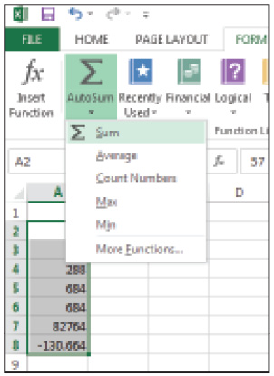
Quickly calculate a range of values with the AutoSum command.

Using common functions

Before we review some of the more commonly-used functions and how to use them, we need to save the worksheet we have been using to experiment with creating formulas.

1 Choose File > Save, and choose Computer.

2 Click the Browse button, navigate to the Excel04lessons folder, name the file excel04_sample, and click Save.

3 Choose File > Close to close the worksheet. We will continue working with the file named excel04_formulas.

SUM

The Sum function adds together the values in a range of cells, as the following steps show.

1 Click in cell B9.

2 Click the arrow next to the AutoSum button in the Editing group of the Home tab, and select Sum from the drop-down menu.

AutoSum button found in the Editing group of the Home tab.

3 Excel automatically selects the range of cells immediately adjacent to the current cell, in this case the values directly above cell B9, or range B5:B8.

Excel automatically selects the range of cells adjacent to the current cell.

4 Press Enter on your keyboard to sum the range.

AVERAGE

The Average function finds the average value in a range of cells, as the following example shows.

1 Click in cell B10.

2 Click the arrow next to the AutoSum button in the Editing group, and select Average from the drop-down menu.

Excel automatically selects the range of cells immediately adjacent to the current cell, in this case the values directly above cell B10, or range B5:B9.

3 Change the range to B5:B8.

4 Press Enter on your keyboard. Excel displays the average amount in cell B10.

MAX

The Max function finds the maximum value in a range of cells, as the following example shows.

1 Click in cell B11.

2 Click the arrow next to the AutoSum button, and select Max from the drop-down menu.

Excel automatically selects the range of cells immediately adjacent to the current cell, in this case the values directly above cell B11, or range B5:B10.

3 Change the range to B5:B8.

4 Press Enter on your keyboard. Excel displays the Maximum value in cell B11.

MIN

The Min function finds the minimum value in a range of cells, as the following example shows.

1 Click in cell B12.

2 Click the arrow next to the AutoSum button and select Min from the drop-down menu.

Excel automatically selects the range of cells immediately adjacent to the current cell, in this case the values directly above cell B12, or range B5:B11.

3 Change the range to B5:B8.

4 Press Enter on your keyboard. Excel displays the minimum value in cell B12.

MEDIAN

The Median function finds the middle value in a range of cells, as shown by the next set of steps.

1 Click in cell B13.

2 Type =MEDIAN(.

3 Select range B5:B8.

4 Type ) and press Enter on your keyboard.

5 Excel displays the median value in cell B13.

IF

The If function performs a logical test on a cell or range of cells to determine whether a specified condition has been met. For example, suppose you have decided that a Bonus will be granted to the individual who sells more than 700 units of certain product. The example below shows how you can use the If function to calculate whether the value in cell B9 meets this criteria.

1 Click in cell B16.

2 Type =IF(B9>700,"Yes","No") and press Enter on the keyboard.

Perform logical tests on data using IF and COUNTIF functions. Here, data is analyzed to see if sales quotas have been met.

Excel evaluates the Total amount in cell B9 to determine whether more than 700 units have been sold (in other words, whether the value in B9 is greater than 700). If the value in B9 is greater than 700, (meaning that more than 700 units have been sold), the formula returns the label Yes, and you can give the individual his or her bonus. However, if the value in B9 is 700 or less, the function returns the label No, and you can decide not to grant the individual his or her bonus.

COUNTIF

COUNTIF is similar to IF in that the function evaluates a cell or range of cells to test for a specific condition. However, the COUNTIF function returns the number of times the condition has been meet in the range, not whether the condition has been met at all. For example, suppose you want to figure out how many brokers have met a sales quota of 200 units. The following set of steps illustrates how to apply the COUNTIF formula to make this determination.

1 Click in cell B17.

2 Type =COUNTIF(B5:B8,">200") and press Enter on the keyboard.

Excel evaluates the values in range B5:B8 to determine how many of the cells within this range have values that are greater than 200 (in other words, how many brokers met the sales quota of 200 units.)

NOW

The NOW function enters the current date and time in a worksheet cell and it’s updated whenever the workbook is opened. An example is shown below.

1 Click in cell G2.

2 From the Formulas tab, choose Date & Time.

3 From the drop-down list that appears, select NOW. Note that the function does not take any arguments.

4 Click OK in the resulting dialog box.

Excel enters the current date and time in cell G2.

PMT

The PMT function calculates the monthly payment amount on a loan. The arguments it uses are the Interest Rate (rate), Term (nper), and Principal (pv) amount. You must adjust the interest rate period and payments to use the same number units. For example, if you make monthly payments on the loan, the interest rate needs to be adjusted to rate/12 and the term or Nper adjusted to nper*12. In the following example, you will calculate the monthly payment for a 30-year loan of $425,000 at a 4.25% interest rate.

1 Click in cell H8.

2 From the Formulas tab, choose Financial.

3 From the list of functions that appears, select PMT.

4 In the Functions Argument dialog box, enter the following: H4/12 in Rate; H5*12 in Nper; and H6 in Pv.

5 Click OK. Excel calculates the monthly payment of -$2,090.74. (The amount is displayed as a negative number to indicate that it is a payment.)

Calculate the monthly payment on a loan using the PMT function.

Working with ranges

You can assign names to particular ranges within a worksheet. By assigning a name to a range, you can more easily describe data. In particular, you can use range names in formulas rather than cell references to describe the data being used in the formula.

For instance, in the worksheet shown in the figure below, range B5:B8 contains data for the number of individual houses sold. If you assign the name House to that range, we can easily construct the formula =SUM(House) to calculates the total number of houses sold.

Naming a range of cells

The following set of steps shows an example of how to name a range of cells.

1 Select range B5:B8.

2 From the Formulas tab, choose Define Name.

3 In the Name box, type House.

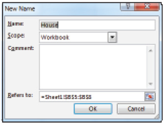
Name a range of cells to describe the data in your worksheet.

4 Click OK.

Naming a range of cells from a selection

You can quickly convert row or column headings to range names. To do so, first select the range of cells to name, including the heading you want to use as the name. Here’s an example.

1 Select range C4:C8.

2 In the Formulas tab, choose Create from Selection. Excel automatically selects Top Row.

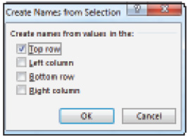
Quickly name a range of cells using existing headings.

3 Click OK. Excel creates the range name Condo for range C5:C8.

4 Select range A5:C8.

5 In the Formulas tab, choose Create from Selection. Excel automatically selects Left column.

6 Click OK. Excel creates range names for each row of broker’s sales.

Using a range name in a formula

When using a name in a formula, you can type the range name or select the name from a list, as the next set of steps illustrates.

1 Click in cell C9.

2 Type =SUM( to begin the formula.

3 From the Formulas tab, choose Use in Formula.

4 From the list that appears, select Condo, and then type ).

Select the Range Name to use in the formula instead of typing the cell addresses.

5 Press Enter. Excel calculates the Total number of Condo units sold.

Editing a range name

You can use the Name Manager in the Formulas tab to adjust the range addresses or to rename your range names. Note that when you rename a range, you must update any formulas that use the range names.

1 From the Formulas tab, choose Name Manager.

The Name Manager is used to modify existing range names.

2 Select the range name Erica and click Edit.

3 Type EricaM in the Name box and click OK.

4 Click Close to close the Name Manager.

Extending a range

Range names automatically adjust to accommodate new cells when you add a cell to an existing range of cells. You will need to extend a range name to include new data if you add that data to the bottom of an existing range.

1 From the Formulas tab, choose Name Manager.

2 Select the range name Danielle.

3 In the Refers to box, edit the range to include column D. (Change the C in the range to a D.)

4 Click the Accept button which looks like a checkmark to the left of the Refers to text box.

5 Click Close to close the Name Manager.

Deleting a range name

The next set of steps shows an example of how to delete range names.

1 From the Formulas tab, choose Name Manager.

2 Select Philip and click Delete.

3 Click OK in the resulting dialog box to confirm the deletion.

4 Click Close to close the Name Manager.

When you delete a range name, any formula that refers to that range name will result in an Error. (The error message #NAME? is returned in the cell.) To correct the error, you must redefine the name or replace the range name in the formula with the appropriate range address.

Copying formulas

After creating a formula in Excel, you can use the Copy and Paste commands to duplicate or transfer the formula in/to other areas of your worksheet. When you copy formulas that contain cell references, the references adjust to their new location, unless you specify otherwise.

Using absolute and relative cell references

When you use cell references in your formulas, Excel uses the data stored in that location in its calculations. The benefit is that when you change the original data, the formula is updated as well.

If you copy a formula from one location to another, Excel adjusts the cell reference based on its new location. For instance, the formula =B2*B3 entered in cell B5 would be adjusted to =C2*C3 when copied to cell C5. However, you can modify the cell reference so it remains fixed to its original location.

An absolute cell reference in a formula remains fixed even when the formulas are copied or moved. A relative cell reference adjusts to its new location.

The dollar sign ($) is used to indicate that the cell reference should remain absolute. Use the dollar sign to indicate the portion of the address (the row reference, the column reference, or both) that should remain fixed. The following table shows some examples.

Absolute and relative cell references
Reference	What it Means
$A6	Column A remains fixed, row 6 adjusts
A$6	Row 6 remains fixed, column A adjusts
$A$6	Cell A6 remains fixed
A6	The reference to column A and row 6 adjusts to its new location

Making a cell reference absolute

The following example shows how to make a cell reference absolute.

1 Type = in cell D5.

2 Point to cell B5 and then press the F4 function key on your keyboard. Excel inserts a dollar sign ($) between the row and column reference.

3 Type + and point to cell C5.

4 Press Enter on the keyboard. The formula in cell D5 now reads =$B$5+C5.

When you use a range name in a formula, Excel automatically makes the range absolute. In other words, when you copy a formula that makes use of a range name, the range reference will not adjust to its new location.

Copying formulas with AutoFill

The AutoFill command lets you quickly copy a formula to a range of adjacent cells. Perform the following set of steps to practice using the AutoFill command.

1 Click in cell D5.

2 From the Formulas tab, choose AutoSum. Excel adds up the cells immediately adjacent to the current cell, which in this case is range B5:C5. Press Enter.

3 Click in cell D5 and drag the AutoFill handle down to cell D9 and release. Excel copies the formula from cell D5 and adjusts the cell references accordingly.

The AutoFill feature lets you quickly copy a formula to adjacent cells.

Copying formulas with Copy and Paste

When you use the Copy command, Excel stores a copy of the selection on the clipboard, allowing you to paste the data multiple times. Perform the following set of steps to practice copying and pasting data.

1 Click in cell B10.

2 From the Home tab, choose Copy from the Clipboard group.

3 Select range C10:D10.

4 Choose Paste from the Clipboard group. Excel pastes the formula from cell B10 and adjusts the cell references accordingly.

You can also press the Enter key on your keyboard to paste the data in a worksheet cell. However, Excel will remove the stored item from the clipboard.

Pasting formula results

With the Paste Values command, you can copy a formula and then paste the results of the formula in another cell. Perform the following set of steps to practice copying and pasting formula results.

1 Select cell H8 and choose Copy from the Home tab.

2 Click in cell I8, choose Paste from the Clipboard group, and then select Paste Special. The Paste Special dialog box appears.

Paste the results of formulas in a separate cell.

3 Select Values from the Paste Special dialog box and click OK. Excel pastes the result of the PMT formula, (2,090.74) in cell I8.

Moving worksheet formulas

Unlike copying a formula, Excel does not adjust cell references when a formula is moved. There are two ways to move a formula in Excel: with the Cut and Paste command, or by dragging and dropping the formula to its new location.

To drag and drop a formula:

1 Select range D4:D10.

2 Position the mouse pointer on the edge of the selected range; when the mouse pointer changes to a four-headed arrow, click and drag the selection to cell E4.

Quickly move a range of cells to a new location with click, drag and drop.

3 Release to drop the range in its new location.

To move a formula with Cut and Paste:

1 Select range E4:E10.

2 From the Home tab, choose Cut. A flashing dashed border appears around the selected range.

3 Click in cell D4 and choose Paste from the Home tab. Excel pastes the selected range.

Formula auditing

When you begin to work with more complex formulas in your worksheets, Excel provides a set of Auditing tools for help you verify cell formulas and to track down errors in syntax or use. When you use the Auditing tools, Excel makes use of Tracer Arrows to show the relationship between cells and the formulas that reference them. The table below details the Auditing tools and the actions they perform.

Excel formula auditing tools
Command	Tool	Action
Trace Precedents		Indicates cells that are referred to in the formula.
Trace Dependents		Indicates cells that are dependent on the formula.
Remove Arrows		Removes the auditing arrows from the worksheet.
Show Formulas		Displays the formulas in the worksheet instead of the results.
Error Checking		Runs through the worksheets looking for errors.
Evaluate Formula		Runs through a formula argument by argument to ensure its accuracy.

Tracing formula precedents

The following is an example of how to trace formula precedents.

1 Click in cell B9 and choose Trace Precedents from the Formula Audition group on the Formulas tab.

Choose Trace Precedents.

Excel overlays a tracer arrow on range B5:B8, showing the cells that are used in the SUM function in cell B9.

Tracing formula dependents

The following is an example of how to trace formula dependents.

1 Click in cell B9 and choose Trace Dependents from the Formulas tab.

Excel overlays a tracer arrow from cell B9 pointing to cell B16; the IF function that relies on data in cell B9 for its conditional formula; and cell D9, which calculates the total amount.

The Trace Precedents and Trace Dependents tools display the relationships between formulas and the cells that the formulas reference.

Removing tracer arrows

Tracer arrows can be removed from the entire worksheet or one at a time from specific cells.

To remove precedent arrows:

1 Click in cell B9 and then click the arrow to the right of the Remove Arrows command on the Formulas tab.

2 Choose Remove Precedent Arrows.

To remove dependent arrows:

1 Click in cell B9 and then click the arrow to the right of the Remove Arrows command on the Formulas tab.

2 Choose Remove Dependent Arrows.

To remove all tracer arrows:

1 From the Formulas tab, choose Remove Arrows.

Viewing formula references

The Tracer Arrows offer a visual display of the relationships between formulas and the cells that reference them, but sometimes the easiest way to view these relationships is to switch to Edit mode. To do so, double-click the cell you want, press the F2 key on your keyboard, or click in the formula bar. When you do, each cell referenced by the formula is displayed.

1 Click in cell H8.

2 Press the F2 key on your keyboard. Alternatively, double-click in the Formula bar or on the cell itself. Excel color-codes each cell referenced by the formula.

When you enter Edit mode, Excel color-codes each cell referenced by the formula.

3 Press Esc on your keyboard to exit Edit mode.

Displaying worksheet formulas

As mentioned previously, Excel displays the result of the formula in a cell rather than the formula itself. With the Show Formulas auditing tool, you can switch the worksheet display so that it displays the formulas as entered.

1 From the Formulas tab, choose Show Formulas. Excel displays all formulas in the cells as entered.

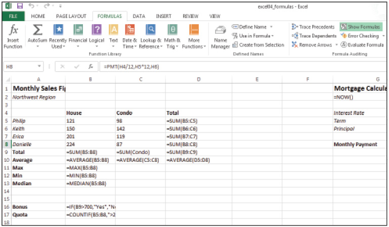
Switch the worksheet view to Show Formulas when you want to view the formulas and not the results.

2 Choose Show Formulas again display the formula results.

3 Choose File > Save As, navigate to the Excel04lessons folder.

4 Type excel04_formulas_final as the file name, and click Save.

You’ve now completed this lesson. Now that you have learned how to work with formulas to perform calculations, you are ready to learn how to produce charts and graphs with your worksheet data, which you will learn in Lesson 5, “Working with Charts.”

Self study

Using the excel04_formulas_final lesson file, complete the following exercises.

1 Calculate the Max, Min, and Median values for Condo units.

2 Update the Principal amount used by the PMT function in cell H8 to $575,000.

3 Copy the formulas in range B16:B17 to cell C16.

Review

Questions

1 What is the difference between relative and absolute cell references, and how do you make a cell reference absolute?

2 What is the quickest way to edit a formula?

3 How do you name a range of cells to use in a formula?

4 What happens when you delete a range name from a worksheet, and how can you fix it?

5 How do you move a range of formulas (or a single formula) from one location to another?

Answers

1 The difference between relative and absolute cell references is that a relative cell reference adjusts to its new location when copied, whereas an absolute cell reference does not. To make a cell reference absolute, enter a dollar sign before each portion of the cell reference. For instance, $G$4 means the reference to cell G4 will not change when copied.

2 The quickest way to edit a formula is to double-click the cell containing the formula you want to edit.

3 To name a range of cells to use in a formula, select the range of cells you want and choose Define Name from the Formulas tab. Enter the name for the range in the resulting dialog box and click OK.

4 When you delete a range name from a worksheet, any formula that references that name will result in an #ERROR. You must update the formula with a new range name reference or enter the appropriate cell references.

5 To move a range of formulas (or a single formula) from one location to another, select the range of cells containing the data you want to move. Point at the selected range, and when the cell pointer changes to a four-headed arrow, click and drag the highlighted border to the new location. Conversely, choose Cut from the Home tab, move to the appropriate cell, and choose Paste.