Chapter 13
Entering and Editing Worksheet Data
IN THIS CHAPTER
Understanding the types of data you can use
Entering text and values into your worksheets, including using the new Flash Fill feature
Entering dates and times into your worksheets
Modifying and editing information
Using built-in number formats
This chapter describes what you need to know about entering and modifying data in your worksheets. As you see, Excel doesn’t treat all data equally. Therefore, you need to learn about the various types of data that you can use in an Excel worksheet.
Exploring Data Types
An Excel workbook file can hold any number of worksheets, and each worksheet is made up of more than 17 billion cells. A cell can hold any of three basic types of data:
- A numeric value
- Text
- A formula
A worksheet can also hold charts, diagrams, pictures, buttons, and other objects. These objects aren’t contained in cells. Instead, they reside on the worksheet’s draw layer, which is an invisible layer on top of each worksheet.
Understanding numeric values
Numeric values represent a quantity of some type: sales amounts, number of employees, atomic weights, test scores, and so on. Values also can be dates (such as Feb-26-2013) or times (such as 3:24 a.m.).
- Largest positive number: 9.9E+307
- Smallest negative number: −9.9E+307
- Smallest positive number: 1E–307
- Largest negative number: −1E–307
Understanding text entries
Most worksheets also include text in some of the cells. Text can serve as data (for example, a list of employee names), labels for values, headings for columns, or instructions about the worksheet. Text is often used to clarify what the values in a worksheet mean or where the numbers came from.
Text that begins with a number is still considered text. For example, if you type 12 Employees into a cell, Excel considers the entry to be text rather than a numeric value. Consequently, you can’t use this cell for numeric calculations. If you need to indicate that the number 12 refers to employees, enter 12 into a cell and then type Employees into the cell to the right.
Understanding formulas
Formulas are what make a spreadsheet a spreadsheet. Excel enables you to enter flexible formulas that use the values (or even text) in cells to calculate a result. When you enter a formula into a cell, the formula’s result appears in the cell. If you change any of the cells used by a formula, the formula recalculates and shows the new result.
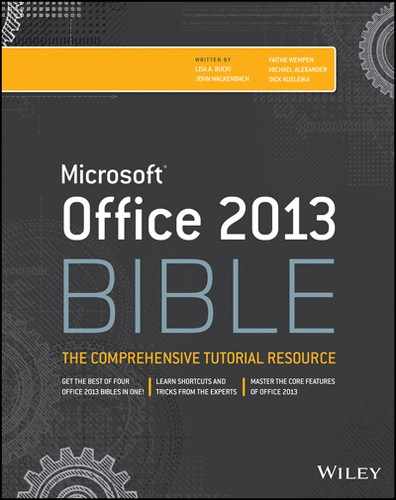
Formulas can be simple mathematical expressions, or they can use some of the powerful functions that are built into Excel. Figure 13.1 shows an Excel worksheet set up to calculate a monthly loan payment. The worksheet contains values, text, and formulas. The cells in column A contain text. Column B contains four values and two formulas. The formulas are in cells B6 and B10. Column D, for reference, shows the actual contents of the cells in column B.
FIGURE 13.1 You can use values, text, and formulas to create useful Excel worksheets.
Entering Text and Values into Your Worksheets
To enter a numeric value into a cell, move the cell pointer to the appropriate cell, type the value, and then press Enter or one of the navigation keys. The value is displayed in the cell and also appears in the Formula bar when the cell is selected. You can include decimal points and currency symbols when entering values, along with plus signs, minus signs, and commas (to separate thousands). If you precede a value with a minus sign or enclose it in parentheses, Excel considers it to be a negative number.
Entering text into a cell is just as easy as entering a value: Activate the cell, type the text, and then press Enter or a navigation key. A cell can contain a maximum of about 32,000 characters — more than enough to hold a typical chapter in this book. Even though a cell can hold a huge number of characters, you’ll find that it’s not possible to actually display all these characters.
FIGURE 13.2 The Formula bar, expanded in height to show more information in the cell

What happens when you enter text that’s longer than its column’s current width? If the cells to the immediate right are blank, Excel displays the text in its entirety, appearing to spill the entry into adjacent cells. If an adjacent cell isn’t blank, Excel displays as much of the text as possible. (The full text is contained in the cell; it’s just not displayed.) If you need to display a long text string in a cell that’s adjacent to a nonblank cell, you have a few choices:
- Edit your text to make it shorter.
- Increase the width of the column (drag the border in the column letter display).
- Use a smaller font.
- Wrap the text within the cell so that it occupies more than one line. Choose Home ⇒ Alignment ⇒ Wrap Text to toggle wrapping on and off for the selected cell or range.
Entering Dates and Times into Your Worksheets
Excel treats dates and times as special types of numeric values. Dates and times are values that are formatted so that they appear as dates or times. If you work with dates and times, you need to understand Excel’s date and time system.
Entering date values
Excel handles dates by using a serial number system. The earliest date that Excel understands is January 1, 1900. This date has a serial number of 1. January 2, 1900, has a serial number of 2, and so on. This system makes it easy to deal with dates in formulas. For example, you can enter a formula to calculate the number of days between two dates.
Most of the time, you don’t have to be concerned with Excel’s serial number date system. You can simply enter a date in a common date format, and Excel takes care of the details behind the scenes. For example, if you need to enter June 1, 2013, you can enter the date by typing June 1, 2013 (or use any of several different date formats). Excel interprets your entry and stores the value 41426, which is the serial number for that date.
Entering time values
When you work with times, you extend Excel’s date serial number system to include decimals. In other words, Excel works with times by using fractional days. For example, the date serial number for June 1, 2013, is 41426. Noon on June 1, 2013 (halfway through the day), is represented internally as 41426.5 because the time fraction is added to the date serial number to get the full date/time serial number.
Again, you normally don’t have to be concerned with these serial numbers or fractional serial numbers for times. Just enter the time into a cell in a recognized format. In this case, type June 1, 2013 12:00.
Modifying Cell Contents
After you enter a value or text into a cell, you can modify it in several ways:
- Delete the cell’s contents.
- Replace the cell’s contents with something else.
- Edit the cell’s contents.
Deleting the contents of a cell
To delete the contents of a cell, just click the cell and press the Delete key. To delete more than one cell, select all the cells that you want to delete and then press Delete. Pressing Delete removes the cell’s contents but doesn’t remove any formatting (such as bold, italic, or a different number format) that you may have applied to the cell.
For more control over what gets deleted, you can choose Home ⇒ Editing ⇒ Clear. This command’s drop-down list has five choices:
- Clear All: Clears everything from the cell — its contents, its formatting, and its cell comment (if it has one)
- Clear Formats: Clears only the formatting and leaves the value, text, or formula
- Clear Contents: Clears only the cell’s contents and leaves the formatting
- Clear Comments: Clears the comment (if one exists) attached to the cell
- Clear Hyperlinks: Removes hyperlinks contained in the selected cells. The text remains, but the cell no longer functions as a clickable hyperlink.
Replacing the contents of a cell
To replace the contents of a cell with something else, just activate the cell and type your new entry, which replaces the previous contents. Any formatting applied to the cell remains in place and is applied to the new content.
You can also replace cell contents by dragging and dropping or by pasting data from the Clipboard. In both cases, the cell formatting will be replaced by the format of the new data. To avoid pasting formatting, choose Home ⇒ Clipboard ⇒ Paste ⇒ Values (V), or Home ⇒ Clipboard ⇒ Paste ⇒ Formulas (F).
Editing the contents of a cell
If the cell contains only a few characters, replacing its contents by typing new data usually is easiest. However, if the cell contains lengthy text or a complex formula and you need to make only a slight modification, you probably want to edit the cell rather than re-enter information.
When you want to edit the contents of a cell, you can use one of the following ways to enter cell-edit mode:
- Double-click the cell to edit the cell contents directly in the cell.
- Select the cell and press F2 to edit the cell contents directly in the cell.
- Select the cell that you want to edit and then click inside the Formula bar to edit the cell contents in the Formula bar.
You can use whichever method you prefer. Some people find editing directly in the cell easier; others prefer to use the Formula bar to edit a cell.
All these methods cause Excel to go into edit mode. (The word Edit appears at the left side of the status bar at the bottom of the screen.) When Excel is in edit mode, the Formula bar enables two icons: Cancel (the X) and Enter (the check mark). Figure 13.3 shows these two icons. Clicking the Cancel icon cancels editing without changing the cell’s contents. (Pressing Esc has the same effect.) Clicking the Enter icon completes the editing and enters the modified contents into the cell. (Pressing Enter has the same effect.)
FIGURE 13.3 While editing a cell, the Formula bar enables two new icons: Cancel (X) and Enter (check mark).

When you begin editing a cell, the insertion point appears as a vertical bar, and you can perform the following tasks:
- Add new characters at the location of the insertion point. Move the insertion point by:
- Using the navigation keys to move within the cell
- Pressing Home to move the insertion point to the beginning of the cell
- Pressing End to move the insertion point to the end of the cell
- Select multiple characters. Press Shift while you use the navigation keys.
- Select characters while you’re editing a cell. Use the mouse. Just click and drag the mouse pointer over the characters that you want to select.
Learning some handy data-entry techniques
You can simplify the process of entering information into your Excel worksheets and make your work go quite a bit faster by using a number of useful tricks, described in the following sections.
Automatically moving the cell pointer after entering data
By default, Excel automatically moves the cell pointer to the next cell down when you press the Enter key after entering data into a cell. (The exception is if you have previously used Tab to make entries across a row; when you press Enter in that case, the cell pointer moves to the next row, in the first column where you entered data in the row above.) To change this setting, choose File ⇒ Options and click the Advanced tab (see Figure 13.4). The check box that controls this behavior is labeled After pressing Enter, move selection. If you enable this option, you can choose the direction in which the cell pointer moves (down, left, up, or right).
FIGURE 13.4 You can use the Advanced tab in Excel Options to select a number of helpful input option settings.

Your choice is completely a matter of personal preference. I prefer to keep this option turned off. When entering data, I use the navigation keys rather than the Enter key (see the next section).
Using navigation keys instead of pressing Enter
Instead of pressing the Enter key when you’re finished making a cell entry, you also can use any of the navigation keys to complete the entry. Not surprisingly, these navigation keys send you in the direction that you indicate. For example, if you’re entering data in a row, press the right-arrow (→) key rather than Enter. The other arrow keys work as expected, and you can even use Page Up and Page Down.
Selecting a range of input cells before entering data
When a range of cells is selected, Excel automatically moves the cell pointer to the next cell in the range when you press Enter. If the selection consists of multiple rows, Excel moves down the column; when it reaches the end of the selection in the column, it moves to the first selected cell in the next column.
To skip a cell, just press Enter without entering anything. To go backward, press Shift+Enter. If you prefer to enter the data by rows rather than by columns, press Tab rather than Enter. Excel continues to cycle through the selected range until you select a cell outside of the range.
Using Ctrl+Enter to place information into multiple cells simultaneously
If you need to enter the same data into multiple cells, Excel offers a handy shortcut. Select all the cells that you want to contain the data, enter the value, text, or formula, and then press Ctrl+Enter. The same information is inserted into each cell in the selection.
Entering decimal points automatically
If you need to enter lots of numbers with a fixed number of decimal places, Excel has a useful tool that works like some old adding machines. Access the Excel Options dialog box and click the Advanced tab. Select the Automatically Insert a Decimal Point check box and make sure that the Places box is set for the correct number of decimal places for the data you need to enter.
When this option is set, Excel supplies the decimal points for you automatically. For example, if you specify two decimal places, entering 12345 into a cell is interpreted as 123.45. To restore things to normal, just clear the Automatically Insert a Decimal Point check box in the Excel Options dialog box. Changing this setting doesn’t affect any values that you already entered.
Using Auto Fill to enter a series of values
The Excel Auto Fill feature makes inserting a series of values or text items in a range of cells easy. It uses the Auto Fill handle (the small box at the lower right of the active cell). You can drag the Auto Fill handle to copy the cell or automatically complete a series.
Figure 13.5 shows an example. I entered 1 into cell A1 and 3 into cell A2. Then I selected both cells and dragged down the fill handle to create a linear series of odd numbers. The figure also shows an icon that, when clicked, displays some additional Auto Fill options.
FIGURE 13.5 This series was created by using Auto Fill.

Using AutoComplete to automate data entry
The Excel AutoComplete feature makes entering the same text into multiple cells easy. With AutoComplete, you type the first few letters of a text entry into a cell, and Excel automatically completes the entry based on other entries that you already made in the column. Besides reducing typing, this feature also ensures that your entries are spelled correctly and are consistent.
Here’s how it works: Suppose that you’re entering product information in a column. One of your products is named Widgets. The first time that you enter Widgets into a cell, Excel remembers it. Later, when you start typing Widgets in that same column, Excel recognizes it by the first few letters and finishes typing it for you. Just press Enter, and you’re done. To override the suggestion, just keep typing.
AutoComplete also changes the case of letters for you automatically. If you start entering widgets (with a lowercase w) in the second entry, Excel makes the w uppercase to be consistent with the previous entry in the column.
Keep in mind that AutoComplete works only within a contiguous column of cells. If you have a blank row, for example, AutoComplete identifies only the cell contents below the blank row.
If you find the AutoComplete feature distracting, you can turn it off by using the Advanced tab of the Excel Options dialog box. Remove the check mark from the check box labeled Enable AutoComplete for cell values.
Forcing text to appear on a new line within a cell
If you have lengthy text in a cell, you can force Excel to display it in multiple lines within the cell: Press Alt+Enter to start a new line in a cell.
When you add a line break, Excel automatically changes the cell’s format to Wrap Text. But unlike normal text wrap, your manual line break forces Excel to break the text at a specific place within the text, which gives you more precise control over the appearance of the text than if you rely on automatic text wrapping.
Using AutoCorrect for shorthand data entry
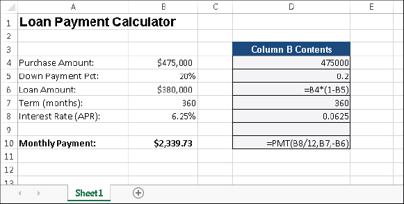
You can use the AutoCorrect feature to create shortcuts for commonly used words or phrases. For example, if you work for a company named Consolidated Data Processing Corporation, you can create an AutoCorrect entry for an abbreviation, such as cdp. Then, whenever you type cdp, Excel automatically changes it to Consolidated Data Processing Corporation.
Excel includes quite a few built-in AutoCorrect terms (mostly to correct common misspellings), and you can add your own. To set up your custom AutoCorrect entries, access the Excel Options dialog box (choose File ⇒ Options) and click the Proofing tab. Then click the AutoCorrect Options button to display the AutoCorrect dialog box. In the dialog box, click the AutoCorrect tab, check the option labeled Replace Text as You Type, and then enter your custom entries. (Figure 13.6 shows an example.) You can set up as many custom entries as you like. Just be careful not to use an abbreviation that might appear normally in your text.
FIGURE 13.6 AutoCorrect allows you to create shorthand abbreviations for text you enter often.
Entering numbers with fractions
To enter a fractional value into a cell, leave a space between the whole number and the fraction. For example, to enter 6 7/8, enter 6 7/8 and then press Enter. When you select the cell, 6.875 appears in the Formula bar, and the cell entry appears as a fraction. If you have a fraction only (for example, 1/8), you must enter a zero first, like this — 0 1/8 — or Excel will likely assume that you’re entering a date. When you select the cell and look at the Formula bar, you see 0.125. In the cell, you see 1/8.
Using a form for data entry
Many people use Excel to manage lists in which the information is arranged in rows. Excel offers a simple way to work with this type of data through the use of a data entry form that Excel can create automatically. This data form works with either a normal range of data, or with a range that has been designated as a table (choose Insert ⇒ Tables ⇒ Table). Figure 13.7 shows an example.
FIGURE 13.7 Excel’s built-in data form can simplify many data-entry tasks.

Unfortunately, the command to access the data form is not on the Ribbon. To use the data form, you must add it to your Quick Access Toolbar or add it to the Ribbon. The following instructions describe how to add this command to your Quick Access Toolbar:
After performing these steps, a new icon appears on your Quick Access Toolbar.
To use a data entry form, follow these steps:
You can also use the form to edit existing data.
Entering the current date or time into a cell
If you need to date-stamp or time-stamp your worksheet, Excel provides two shortcut keys that do this task for you:
- Current date: Ctrl+; (semicolon)
- Current time: Ctrl+Shift+; (semicolon)
The date and time are from the system time in your computer. If the date or time isn’t correct in Excel, use the Windows Control Panel to make the adjustment.
=TODAY()
=NOW()
Using Flash Fill
The Text to Columns Wizard works well for many types of data. But sometimes you’ll encounter data that can’t be parsed by that wizard. For example, the Text to Columns Wizard is useless if you have variable-width data that doesn’t have delimiters. In such a case, the Flash Fill feature might save the day. But keep in mind that Flash Fill works successfully only when the data is very consistent.
Flash Fill uses pattern recognition to extract data (and also concatenate data). Just enter a few examples in a column that’s adjacent to the data, and choose Data ⇒ Data Tools ⇒ Flash Fill (or press Ctrl+E). Excel analyzes the examples and attempts to fill in the remaining cells. If Excel didn’t recognize the pattern you had in mind, press Ctrl+Z, add another example or two, and try again.
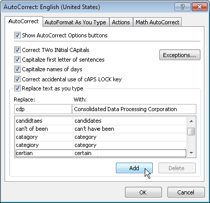
Figure 13.8 shows a worksheet with some text in a single column. The goal is to extract the number from each cell and put it into a separate cell. The Text to Columns Wizard can’t do it because the space delimiters aren’t consistent. It might be possible to write an array formula, but it would be very complicated.
FIGURE 13.8 The goal is to extract the numbers in column A.
To try using Flash Fill, activate cell B1 and type the first number (20). Move to B2, and type the second number (6). Can Flash Fill identify the remaining numbers and fill them in? Choose Data ⇒ Data Tools ⇒ Flash Fill or Home ⇒ Editing ⇒ Fill ⇒ Flash Fill (or press Ctrl+E) and Excel fills in the remaining cells in a flash. Figure 13.9 shows the result.
FIGURE 13.9 Using manually entered examples in B1 and B2, Excel makes some incorrect guesses.

As you see, Excel identified most of the values. Accuracy increases if you provide more examples. For example, provide an example of a decimal number. Delete the suggested values, enter 3.12 in cell B6, and press Ctrl+E. This time, Excel gets them all correct (see Figure 13.10).
FIGURE 13.10 After you enter an example of a decimal number, Excel gets them all correct.

This simple example demonstrates two important points:
- You must examine your data very carefully after using Flash Fill. Just because the first few rows are correct, you can’t assume that Flash Fill worked correctly for all rows.
- Flash Fill increases accuracy when you provide more examples.
Figure 13.11 shows another example, names in column A. The goal is to extract the first, last, and middle name (if it has one). In column B Excel successfully gets all the first names using only two examples (Mark and Tim). Plus, it successfully extracted all the last names (column C), using Russell and Colman. Extracting the middle names or initials (column D) eluded me until I provided examples that included a space on either side of the middle name).
FIGURE 13.11 Using Flash Fill to split names

To summarize, Excel’s new Flash Fill is an interesting idea, but it seems to work reliably only if the data is very consistent. Even when you think it worked correctly, make sure you examine the results carefully. And think twice before trusting it with important data. There’s no way to document how the data was extracted. But the main limitation is that (unlike formulas) Flash Fill is not a dynamic technique. If your data changes, the flash-filled column does not update.
Applying Number Formatting
Number formatting refers to the process of changing the appearance of values contained in cells. Excel provides a wide variety of number formatting options. In the following sections, you see how to use many of Excel’s formatting options to quickly improve the appearance of your worksheets.
Values that you enter into cells normally are unformatted. In other words, they simply consist of a string of numerals. Typically, you want to format the numbers so that they’re easier to read or are more consistent in terms of the number of decimal places shown.
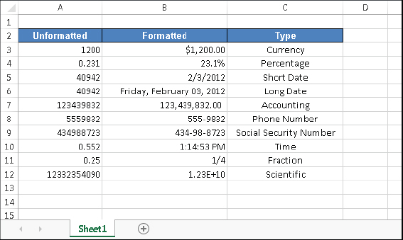
Figure 13.12 shows a worksheet that has two columns of values. The first column consists of unformatted values. The cells in the second column are formatted to make the values easier to read. The third column describes the type of formatting applied.
FIGURE 13.12 Use numeric formatting to make it easier to understand what the values in the worksheet represent.
Using automatic number formatting
Excel is smart enough to perform some formatting for you automatically. For example, if you enter 12.2% into a cell, Excel knows that you want to use a percentage format and applies it for you automatically. If you use commas to separate thousands (such as 123,456), Excel applies comma formatting for you. And if you precede your value with a dollar sign, the cell is formatted for currency (assuming that the dollar sign is your system currency symbol).
Formatting numbers by using the Ribbon
The Home ⇒ Number group in the Ribbon contains controls that let you quickly apply common number formats (see Figure 13.13).
FIGURE 13.13 You can find number formatting commands in the Number group of the Home tab.

The Number Format drop-down list contains several common number formats. Additional options include an Accounting Number Format drop-down list (to select a currency format), a Percent Style button, and a Comma Style button. The group also contains a button to increase the number of decimal places, and another to decrease the number of decimal places.
When you select one of these controls, the active cell takes on the specified number format. You also can select a range of cells (or even an entire row or column) before clicking these buttons. If you select more than one cell, Excel applies the number format to all the selected cells.
Using keyboard shortcuts to format numbers
Another way to apply number formatting is to use keyboard shortcuts. Table 13.1 summarizes the keyboard shortcut combinations that you can use to apply common number formatting to the selected cells or range. Notice that these Ctrl+Shift characters are all located together, in the upper left of your keyboard.
TABLE 13.1 Number Formatting Keyboard Shortcuts
| Key Combination | Formatting Applied |
| Ctrl+Shift+~ | General number format (that is, unformatted values) |
| Ctrl+Shift+$ | Currency format with two decimal places (negative numbers appear in parentheses) |
| Ctrl+Shift+% | Percentage format, with no decimal places |
| Ctrl+Shift+^ | Scientific notation number format, with two decimal places |
| Ctrl+Shift+# | Date format with the day, month, and year |
| Ctrl+Shift+@ | Time format with the hour, minute, and AM or PM |
| Ctrl+Shift+! | Two decimal places, thousands separator, and a hyphen for negative values |
Formatting numbers using the Format Cells dialog box
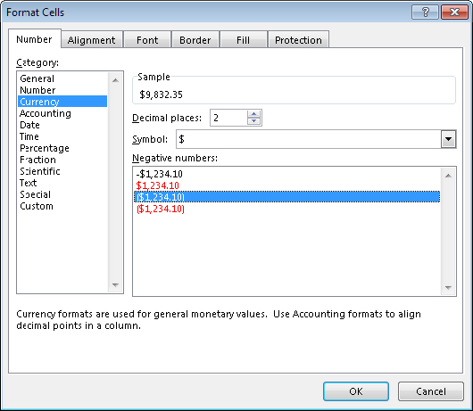
In most cases, the number formats that are accessible from the Number group on the Home tab are just fine. Sometimes, however, you want more control over how your values appear. Excel offers a great deal of control over number formats through the use of the Format Cells dialog box, shown in Figure 13.14. For formatting numbers, you need to use the Number tab.
FIGURE 13.14 When you need more control over number formats, use the Number tab of the Format Cells dialog box.
You can bring up the Format Cells dialog box in several ways. Start by selecting the cell or cells that you want to format and then do one of the following:
- Choose Home and click the dialog box launcher in the lower-right corner of the Number group.
- Choose Home ⇒ Number, click the Number Format drop-down list, and choose More Number Formats from the drop-down list.
- Right-click the cell and choose Format Cells from the shortcut menu.
- Press Ctrl+1.
The Number tab of the Format Cells dialog box displays 12 categories of number formats. When you select a category from the list box, the right side of the tab changes to display options appropriate to that category.
The Number category has three options that you can control: the number of decimal places displayed, whether to use a thousands separator, and how you want negative numbers displayed. Notice that the Negative Numbers list box has four choices (two of which display negative values in red), and the choices change depending on the number of decimal places and whether you choose to separate thousands.
The top of the tab displays a sample of how the active cell will appear with the selected number format (visible only if a cell with a value is selected). After you make your choices, click OK to apply the number format to all the selected cells.
The following are the number format categories, along with some general comments:
- General: The default format; it displays numbers as integers, as decimals, or in scientific notation if the value is too wide to fit in the cell.
- Number: Enables you to specify the number of decimal places, whether to use a comma to separate thousands, and how to display negative numbers (with a minus sign, in red, in parentheses, or in red and in parentheses)
- Currency: Enables you to specify the number of decimal places, choose a currency symbol, and how to display negative numbers (with a minus sign, in red, in parentheses, or in red and in parentheses). This format always uses a comma to separate thousands.
- Accounting: Differs from the Currency format in that the currency symbols always align vertically
- Date: Enables you to choose from several different date formats
- Time: Enables you to choose from several different time formats
- Percentage: Enables you to choose the number of decimal places and always displays a percent sign
- Fraction: Enables you to choose from among nine fraction formats
- Scientific: Displays numbers in exponential notation (with an E): 2.00E+05 = 200,000; 2.05E+05 = 205,000. You can choose the number of decimal places to display to the left of E. The second example can be read as “2.05 times 10 to the fifth.”
- Text: When applied to a value, causes Excel to treat the value as text (even if it looks like a number). This feature is useful for such items as part numbers and credit card numbers.
- Special: Contains additional number formats. In the U.S. version of Excel, the additional number formats are Zip Code, Zip Code +4, Phone Number, and Social Security Number.
- Custom: Enables you to define custom number formats that aren’t included in any other category
Summary
This chapter showed you the techniques you need to know to enter the contents for any worksheet in Excel. You learned how Excel treats different types of information—text, numbers, and formulas. You can continue on to learn to use ranges, because at this point, you should be able to do the following:
- Enter numeric, text, date, and time values.
- Erase, replace, and edit cell contents.
- Take advantage of a variety of shortcuts for entering data, including Auto Fill, AutoComplete, and Flash Fill.
- Apply number formatting to ensure your data is easy to interpret.