Chapter 12
Using Excel Worksheets and Workbooks
IN THIS PART
Understanding what Excel is used for
Looking at what’s new in Excel 2013
Learning the parts of an Excel window
Navigating Excel worksheets
Introducing Excel’s Ribbon
Trying out Excel with a step-by-step hands-on session
This chapter is an introductory overview of Excel 2013. If you’re already familiar with a previous version of Excel, reading (or at least skimming) this chapter is still a good idea.
Identifying What Excel Is Good For
Excel, as you probably know, is the world’s most widely used spreadsheet software and part of the Microsoft Office suite. Other spreadsheet software is available, but Excel is by far the most popular and has been the world standard for many years.
Much of the appeal of Excel is due to the fact that it’s so versatile. Excel’s forte, of course, is performing numerical calculations, but Excel is also very useful for non-numeric applications. Here are just a few of the uses for Excel:
- Number crunching: Create budgets, tabulate expenses, analyze survey results, and perform just about any type of financial analysis you can think of.
- Creating charts: Create a wide variety of highly customizable charts.
- Organizing lists: Use the row-and-column layout to store lists efficiently.
- Text manipulation: Clean up and standardize text-based data.
- Accessing other data: Import data from a wide variety of sources.
- Creating graphical dashboards: Summarize a large amount of business information in a concise format.
- Creating graphics and diagrams: Use Shapes and SmartArt to create professional-looking diagrams.
- Automating complex tasks: Perform a tedious task with a single mouse click with Excel’s macro capabilities.
Seeing What’s New in Excel 2013
When a new version of Microsoft Office is released, sometimes Excel gets lots of new features and other times it gets very few new features. In the case of Office 2013, Excel got quite a few new features.
Here’s a quick summary of what’s new in Excel 2013, relative to Excel 2010:
- Cloud storage: Excel is tightly integrated with Microsoft’s SkyDrive web-based storage.
- Support for other devices: Excel is available for other devices, including touch-sensitive devices such as Windows RT tablets and Windows phones.
- New aesthetics: Excel has a new “flat” look and displays an (optional) graphic in the title bar. The default color scheme is white, but you can choose from two other color schemes (light gray and dark gray) in the General tab of the Excel Options dialog box.
- Single document interface: Excel no longer supports the option to display multiple workbooks in a single window. Each workbook has its own top-level Excel window and Ribbon.
- New types of assistance: Excel provides recommended PivotTables and recommended charts.
- Flash Fill: Flash Fill is a new way to extract (by example) relevant data from text strings. You can also use this feature to combine data in multiple columns.
- Support for Apps for Office: You can download or purchase apps that can be embedded in a workbook file.
- The Data Model: Create PivotTables from multiple data tables, combined in a relational manner.
- New Slicer option: The Slicer feature, introduced in Excel 2010 for use with PivotTables, has been expanded and now works with tables.
- Timeline filtering: Similar to the Slicer, the Timeline makes it easy to filter data by dates.
- Quick Analysis: Quick Analysis provides single click access to various data analysis tools.
- Enhanced chart formatting: Modifying charts is significantly easier.
- New worksheet functions: Excel 2013 supports dozens of new worksheet functions.
- Backstage: The Backstage screen has been reorganized and is easier to use.
- New add-ins: Three new add-ins are included (for Office Professional Plus only): PowerPivot, Power View, and Inquire.
Understanding Workbooks and Worksheets
The work you do in Excel is performed in a workbook file. You can have as many workbooks open as you need, and each one appears in its own window. By default, Excel workbooks use an .xlsx file extension.
Each workbook contains one or more worksheets, and each worksheet is made up of individual cells. Each cell can contain a value, a formula, or text. A worksheet also has an invisible draw layer, which holds charts, images, and diagrams. Each worksheet in a workbook is accessible by clicking the tab at the bottom of the workbook window. In addition, a workbook can store chart sheets; a chart sheet displays a single chart and is also accessible by clicking a tab.
Newcomers to Excel are often intimidated by all the different elements that appear within Excel’s window. After you become familiar with the various parts, it all starts to make sense, and you’ll feel right at home.
Figure 12.1 shows you the more important bits and pieces of Excel. As you look at the figure, refer to Table 12.1 for a brief explanation of the items shown in the figure.
FIGURE 12.1 The Excel screen has many useful elements that you will use often.
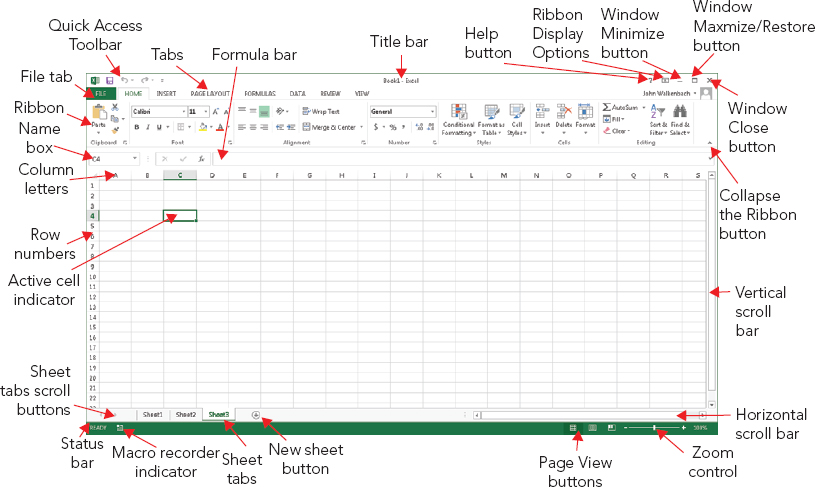
TABLE 12.1 Parts of the Excel Screen That You Need to Know
| Name | Description |
| Active cell indicator | This dark outline indicates the currently active cell (one of the 17,179,869,184 cells on each worksheet). |
| Collapse the Ribbon button | Click this button to temporarily hide the Ribbon. Click it again to make the Ribbon remain visible. |
| Column letters | Letters range from A to XFD — one for each of the 16,384 columns in the worksheet. You can click a column heading to select an entire column of cells or drag a column border to change its width. |
| File tab | Click this button to open Backstage view, which contains many options for working with your document (including printing) and setting Excel options. |
| Formula bar | When you enter information or formulas into a cell, it appears in this bar. |
| Help button | Click this button to display the Excel Help system window. |
| Horizontal scroll bar | Use this tool to scroll the sheet horizontally. |
| Macro recorder indicator | Click to start recording a VBA macro. The icon changes while your actions are being recorded. Click again to stop recording. |
| Name box | This box displays the active cell address or the name of the selected cell, range, or object. |
| New sheet button | Add a new worksheet by clicking the New sheet button (which is displayed after the last sheet tab). |
| Page View buttons | Click these buttons to change the way the worksheet is displayed. |
| Quick Access Toolbar | This customizable toolbar holds commonly used commands. The Quick Access Toolbar is always visible, regardless of which tab is selected. |
| Ribbon | This is the main location for Excel commands. Clicking an item in the tab list changes the Ribbon that is displayed. |
| Ribbon Display Options | A drop-down control that offers three options related to displaying the Ribbon. |
| Row numbers | Numbers range from 1 to 1,048,576 — one for each row in the worksheet. You can click a row number to select an entire row of cells. |
| Sheet tabs | Each of these notebook-like tabs represents a different sheet in the workbook. A workbook can have any number of sheets, and each sheet has its name displayed in a sheet tab. |
| Sheet tab scroll buttons | Use these buttons to scroll the sheet tabs to display tabs that aren’t visible. You can also right-click to get a list of sheets. |
| Status bar | This bar displays various messages, as well as the status of the Num Lock, Caps Lock, and Scroll Lock keys on your keyboard. It also shows summary information about the range of cells selected. Right-click the status bar to change the information displayed. |
| Tabs | Click these tabs to display different Ribbon commands, similar to a menu. |
| Title bar | This displays the name of the program and the name of the current workbook. It also by default holds the Quick Access Toolbar (on the left) and some control buttons that you can use to modify the window (on the right). |
| Vertical scroll bar | Use this to scroll the sheet vertically. |
| Window Close button | Click this button to close the active workbook window. |
| Window Maximize/Restore button | Click this button to increase the workbook window’s size to fill the entire screen. If the window is already maximized, clicking this button returns Excel’s window to its prior size so that it no longer fills the entire screen. |
| Window Minimize button | Click this button to minimize the workbook window. The window displays as an icon in the Windows taskbar. |
| Zoom control | Use this to zoom your worksheet in and out. |
Moving around a Worksheet
This section describes various ways to navigate the cells in a worksheet.
Every worksheet consists of rows (numbered 1 through 1,048,576) and columns (labeled A through XFD). Column labeling works like this: After column Z comes column AA, which is followed by AB, AC, and so on. After column AZ comes BA, BB, and so on. After column ZZ is AAA, AAB, and so on.
The intersection of a row and a column is a single cell, and each cell has a unique address made up of its column letter and row number. For example, the address of the upper-left cell is A1. The address of the cell at the lower right of a worksheet is XFD1048576.
At any given time, one cell is the active cell. The active cell is the cell that accepts keyboard input, and its contents can be edited. You can identify the active cell by its darker border, as shown in Figure 12.2. Its address appears in the Name box. Depending on the technique that you use to navigate through a workbook, you may or may not change the active cell when you navigate.
FIGURE 12.2 The active cell is the cell with the dark border — in this case, cell C8.

Notice that the row and column headings of the active cell appear in a different color to make it easier to identify the row and column of the active cell.
Navigating with your keyboard
Not surprisingly, you can use the standard navigational keys on your keyboard to move around a worksheet. These keys work just as you’d expect: The down arrow moves the active cell down one row, the right arrow moves it one column to the right, and so on. Page Up and Page Down move the active cell up or down one full window. (The actual number of rows moved depends on the number of rows displayed in the window.)
The Num Lock key on your keyboard controls how the keys on the numeric keypad behave. When Num Lock is on, the keys on your numeric keypad generate numbers. Many keyboards have a separate set of navigation (arrow) keys located to the left of the numeric keypad. The state of the Num Lock key doesn’t affect these keys.
Table 12.2 summarizes all the worksheet movement keys available in Excel.
TABLE 12.2 Excel Worksheet Movement Keys
| Key | Action |
| Up Arrow | Moves the active cell up one row |
| Down Arrow | Moves the active cell down one row |
| Left Arrow or Shift+Tab | Moves the active cell one column to the left |
| Right Arrow or Tab | Moves the active cell one column to the right |
| Page Up | Moves the active cell up one screen |
| Page Down | Moves the active cell down one screen |
| Alt+Page Down | Moves the active cell right one screen |
| Alt+Page Up | Moves the active cell left one screen |
| Ctrl+Backspace | Scrolls the screen so that the active cell is visible |
| Ctrl+End | Moves the active cell to the intersection of the row with the lowermost entry (highest row number) on the worksheet and the column with the rightmost entry (highest column letter) on the worksheet |
| Up Arrow | Scrolls the screen up one row (active cell does not change) |
| Down Arrow | Scrolls the screen down one row (active cell does not change) |
| Left Arrow | Scrolls the screen left one column (active cell does not change) |
| Right Arrow | Scrolls the screen right one column (active cell does not change) |
∗ With Scroll Lock on
Navigating with your mouse
To change the active cell by using the mouse, just click another cell, and it becomes the active cell. If the cell that you want to activate isn’t visible in the workbook window, you can use the scroll bars to scroll the window in any direction. To scroll one cell, click either of the arrows on the scroll bar. To scroll by a complete screen, click either side of the scrollbar’s scroll box. You can also drag the scroll box for faster scrolling.
Press Ctrl while you use the mouse wheel to zoom the worksheet. If you prefer to use the mouse wheel to zoom the worksheet without pressing Ctrl, choose File ⇒ Options and select the Advanced section. Under Editing options, click the Zoom on roll with IntelliMouse check box to check it.
Using the scroll bars or scrolling with your mouse doesn’t change the active cell. It simply scrolls the worksheet. To change the active cell, you must click a new cell after scrolling.
Introducing Excel’s Ribbon Tabs
In Office 2007, Microsoft made a dramatic change to the user interface. Traditional menus and toolbars were replaced with the Ribbon, a collection of icons at the top of the screen. The words above the icons are known as tabs: the Home tab, the Insert tab, and so on. Most users find that the Ribbon is easier to use than the old menu system; it can also be customized to make it even easier to use (see Appendix A, “Customizing Office.”).
The Ribbon can either be hidden or visible (it’s your choice). To toggle the Ribbon’s visibility, press Ctrl+F1 (or double-click a tab at the top). If the Ribbon is hidden, it temporarily appears when you click a tab and hides itself when you click in the worksheet. The title bar has a control named Ribbon Display Options (next to the Help button). Click the control and choose one of three Ribbon options: Auto-hide Ribbon, Show Tabs, or Show Tabs and Commands.
Ribbon tabs
The commands available in the Ribbon vary, depending upon which tab is selected. The Ribbon is arranged into groups of related commands. Here’s a quick overview of Excel’s tabs:
- Home: You’ll probably spend most of your time with the Home tab selected. This tab contains the basic Clipboard commands, formatting commands, style commands, commands to insert and delete rows or columns, plus an assortment of worksheet editing commands.
- Insert: Select this tab when you need to insert something in a worksheet — a table, a diagram, a chart, a symbol, and so on.
- Page Layout: This tab contains commands that affect the overall appearance of your worksheet, including some settings that deal with printing.
- Formulas: Use this tab to insert a formula, name a cell or a range, access the formula auditing tools, or control how Excel performs calculations.
- Data: Excel’s data-related commands are on this tab, including data validation commands.
- Review: This tab contains tools to check spelling, translate words, add comments, or protect sheets.
- View: The View tab contains commands that control various aspects of how a sheet is viewed. Some commands on this tab are also available in the status bar.
- Developer: This tab isn’t visible by default. It contains commands that are useful for programmers. To display the Developer tab, choose File ⇒ Options and then select Customize Ribbon. In the Customize the Ribbon section on the right, make sure Main Tabs is selected in the drop-down control, and place a check mark next to Developer.
- Add-Ins: This tab is visible only if you loaded an older workbook or add-in that customizes the menu or toolbars. Because menus and toolbars are no longer available in Excel 2013, these user interface customizations appear on the Add-Ins tab.
The preceding list contains the standard Ribbon tabs. Excel may display additional Ribbon tabs, resulting from add-ins or macros.
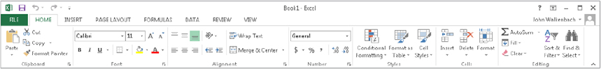
The appearance of the commands on the Ribbon varies, depending on the width of the Excel window. When the Excel window is too narrow to display everything, the commands adapt; some of them might seem to be missing, but the commands are still available. Figure 12.3 shows the Home tab of the Ribbon with all controls fully visible. When you make the Excel window narrower or reduce your screen resolution, some groups display as a single button; however, if you click the button, all the group commands are available to you.
FIGURE 12.3 The Home tab of the Ribbon in Excel.
Contextual tabs
In addition to the standard tabs, Excel also includes contextual tabs. Whenever an object (such as a chart, a table, or a SmartArt diagram) is selected, specific tools for working with that object are made available in the Ribbon.
Figure 12.4 shows the contextual tabs that appear when a chart is selected. In this case, it has two contextual tabs: Chart Tools ⇒ Design and Chart Tools ⇒ Format. When contextual tabs appear, you can, of course, continue to use all the other tabs.
FIGURE 12.4 When you select an object, contextual tabs contain tools for working with that object.

Creating Your First Excel Workbook
This section presents an introductory hands-on session with Excel. If you haven’t used Excel, you may want to follow along on your computer to get a feel for how this software works.
In this example, you create a simple monthly sales projection table along with a chart.
Getting started on your worksheet
Start Excel and make sure that you have an empty workbook displayed by selecting Blank workbook from the Start screen. To create a new, blank workbook when Excel is already open, press Ctrl+N (the shortcut key for File ⇒ New ⇒ Blank Workbook).
The sales projection will consist of two columns of information. Column A will contain the month names, and column B will store the projected sales numbers. You start by entering some descriptive titles into the worksheet. Here’s how to begin:
Filling in the month names
In this step, you enter the month names in column A.
Your worksheet should resemble the one shown in Figure 12.5.
FIGURE 12.5 Your worksheet, after entering the column headings and month names

Entering the sales data
Next, you provide the sales projection numbers in column B. Assume that January’s sales are projected to be $50,000, and that sales will increase by 3.5 percent in each subsequent month.
At this point, your worksheet should resemble the one shown in Figure 12.6. Keep in mind that, except for cell B2, the values in column B are calculated with formulas. To demonstrate, try changing the projected sales value for the initial month, January (in cell B2). You’ll find that the formulas recalculate and return different values. These formulas all depend on the initial value in cell B2, though.
FIGURE 12.6 Your worksheet, after creating the formulas

Formatting the numbers
The values in the worksheet are difficult to read because they aren’t formatted. In this step, you apply a number format to make the numbers easier to read and more consistent in appearance:
Making your worksheet look a bit fancier
At this point, you have a functional worksheet, but it could use some help in the appearance department. Converting this range to an “official” (and attractive) Excel table is a snap:
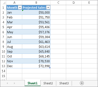
Your worksheet should look like Figure 12.7.
FIGURE 12.7 Your worksheet, after converting the range to a table
If you don’t like the default table style, just select another one from the Table Tools ⇒ Design ⇒ Table Styles group. Notice that you can get a preview of different table styles by moving your mouse over the Ribbon. When you find one you like, click it, and the style will be applied to your table.
Summing the values
The worksheet displays the monthly projected sales, but what about the total projected sales for the year? Because this range is a table, it’s simple:
Creating a chart
How about a chart that shows the projected sales for each month?
Figure 12.8 shows the worksheet with a column chart. Your chart may look different, depending on the chart style you selected.
FIGURE 12.8 The table and chart

Printing your worksheet
Printing your worksheet is very easy (assuming that you have a printer attached and that it works properly).
FIGURE 12.9 Viewing the worksheet in Page Layout view

Saving your workbook
Until now, everything that you’ve done has occurred in your computer’s memory. If the power should fail, all may be lost — unless Excel’s AutoRecover feature happened to kick in. It’s time to save your work to a file on your hard drive.
If you’ve followed along, you may have realized that creating this workbook was not difficult. But, of course, you’ve barely scratched the surface of Excel. The remainder of this book covers these tasks (and many, many more) in much greater detail.
Summary
This chapter touched on the new features of the Excel 2013 spreadsheet program, as well as a few basics to get you started. At this point, you should be able to:
- Name a few ways to use Excel.
- Talk about some of Excel’s exciting new features.
- Understand the difference between a workbook and worksheet.
- Move around a worksheet with the mouse or keyboard.
- Work with the Ribbon.
- Create and save an example workbook file.