Chapter 14
Essential Worksheet and Cell Range Operations
IN THIS CHAPTER
Understanding Excel worksheet essentials
Controlling your views
Manipulating rows and columns
Understanding Excel cells and ranges
Selecting cells and ranges
Copying or moving ranges
Using names to work with ranges
Adding comments to cells
This chapter covers some basic information regarding workbooks, worksheets, and windows. You’ll discover tips and techniques to help you take control of your worksheets and help you work more efficiently. Most of the work you do in Excel involves cells and ranges. Understanding how best to manipulate cells and ranges will save you time and effort, as you’ll also learn in this chapter.
Learning the Fundamentals of Excel Worksheets
In Excel, each file is called a workbook, and each workbook can contain one or more worksheets. You may find it helpful to think of an Excel workbook as a notebook and worksheets as pages in the notebook. As with a notebook, you can view a particular sheet, add new sheets, remove sheets, rearrange sheets, and copy sheets. The following sections describe the operations that you can perform with worksheets.
Working with Excel windows
Each Excel workbook file that you open is displayed in a window. A workbook can hold any number of sheets, and these sheets can be either worksheets (sheets consisting of rows and columns) or chart sheets (sheets that hold a single chart). A worksheet is what people usually think of when they think of a spreadsheet. You can open as many Excel workbooks as necessary at the same time.
Each Excel window has five buttons (which appear as icons) at the right side of its title bar. From left to right, they are Help, Full Screen Mode (or Exit Full Screen Mode), Minimize, Maximize (or Restore Down), and Close.
An Excel window can be in one of the following states:
- Maximized: Fills the entire screen. To maximize a window, click its Maximize button.
- Minimized: Hidden, but still open. To minimize a window, click its Minimize button.
- Restored: A nonmaximized size. To restore a maximized window, click its Restore Down button. To restore a minimized window, click its icon in the Windows taskbar. A window in this state can be resized and moved.
If you work with more than one workbook simultaneously (which is quite common), you need to know how to move, resize, and switch among the workbook windows.
Moving and resizing windows
To move or resize a window, make sure that it’s not maximized (click the Restore Down button). Then drag its title bar with your mouse.
To resize a window, drag any of its borders until it’s the size that you want it to be. When you position the mouse pointer on a window’s border, the mouse pointer changes to a double-headed arrow, which lets you know that you can now drag to resize the window. To resize a window horizontally and vertically at the same time, drag any of its corners.
If you want all your workbook windows to be visible (that is, not obscured by another window), you can move and resize the windows manually, or you can let Excel do it for you. Choosing View ⇒ Window ⇒ Arrange All displays the Arrange Windows dialog box, shown in Figure 14.1. This dialog box has four window arrangement options. Just select the one that you want and click OK. Windows that are minimized aren’t affected by this command.
FIGURE 14.1 Use the Arrange Windows dialog box to quickly arrange all open nonminimized workbook windows.

Switching among windows
At any given time, one (and only one) workbook window is the active window. The active window accepts your input and is the window on which your commands work. The active window appears at the top of the stack of windows. To work in a workbook in a different window, you need to make that window active. You can make a different window the active window in several ways:
- Click another window, if it’s visible. The window you click moves to the top and becomes the active window. This method isn’t possible if the current window is maximized.
- Press Ctrl+F6 to cycle through all open windows until the window that you want to work with appears on top as the active window. Pressing Shift+Ctrl+F6 cycles through the windows in the opposite direction.
- Choose View ⇒ Window ⇒ Switch Windows and select the window that you want from the drop-down list (the active window has a check mark next to it). This menu can display as many as nine windows. If you have more than nine workbook windows open, choose More Windows (which appears below the nine window names).
- Click the Excel icon in the Windows taskbar. You can then choose the window by clicking its thumbnail or clicking it in the pop-up list.
Most people prefer to do most of their work with maximized workbook windows, which enables you to see more cells and eliminates the distraction of other workbook windows getting in the way. At times, however, viewing multiple windows is preferred. For example, displaying two windows is more efficient if you need to compare information in two workbooks or if you need to copy data from one workbook to another.
Closing windows
If you have multiple windows open, you may want to close those windows that you no longer need. Excel offers several ways to close the active window:
- Choose File ⇒ Close.
- Click the Close button (the X icon) on the workbook window’s title bar.
- Press Alt+F4.
- Press Ctrl+W.
When you close a workbook window, Excel checks whether you made any changes since the last time you saved the file. If you have made changes, Excel prompts you to save the file before it closes the window. If not, the window closes without a prompt from Excel. Oddly, Excel provides no way to tell you if a workbook has been changed since it was last saved.
Activating a worksheet
At any given time, one workbook is the active workbook, and one sheet is the active sheet in the active workbook. To activate a different sheet, just click its sheet tab, located at the bottom of the workbook window. You also can use the following shortcut keys to activate a different sheet:
- Ctrl+PageUp: Activates the previous sheet, if one exists
- Ctrl+PageDown: Activates the next sheet, if one exists
If your workbook has many sheets, all its tabs may not be visible. Use the tab scrolling controls (see Figure 14.2) to scroll the sheet tabs. The sheet tabs share space with the worksheet’s horizontal scrollbar. You also can drag the tab split control (to the left of the horizontal scrollbar) to display more or fewer tabs. Dragging the tab split control simultaneously changes the number of tabs and the size of the horizontal scrollbar.
FIGURE 14.2 Use the tab scrolling controls to activate a different worksheet or to see additional worksheet tabs.

Adding a new worksheet to your workbook
Worksheets can be an excellent organizational tool. Instead of placing everything on a single worksheet, you can use additional worksheets in a workbook to separate various workbook elements logically. For example, if you have several products whose sales you track individually, you may want to assign each product to its own worksheet and then use another worksheet to consolidate your results.
Here are three ways to add a new worksheet to a workbook:
- Click the New Sheet button, which is the plus sign icon located to the right of the last sheet tab. A new sheet is added after the active sheet.
- Press Shift+F11. A new sheet is added before the active sheet.
- Right-click a sheet tab, choose Insert from the shortcut menu, and select the General tab of the Insert dialog box that appears. Then select the Worksheet icon and click OK. A new sheet is added before the active sheet.
Deleting a worksheet you no longer need
If you no longer need a worksheet, or if you want to get rid of an empty worksheet in a workbook, you can delete it in either of two ways:
- Right-click its sheet tab and choose Delete from the shortcut menu.
- Activate the unwanted worksheet and choose Home ⇒ Cells ⇒ Delete ⇒ Delete Sheet.
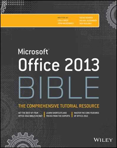
If the worksheet contains any data, Excel asks you to confirm that you want to delete the sheet (see Figure 14.3). If you’ve never used the worksheet, Excel deletes it immediately without asking for confirmation.
FIGURE 14.3 Excel’s gentle warning that you might be losing some data
Changing the name of a worksheet
The default names that Excel uses for worksheets — Sheet1, Sheet2, and so on — are generic and nondescriptive. To make it easier to locate data in a multisheet workbook, you’ll want to make the sheet names more descriptive.
To change a sheet’s name, double-click the sheet tab. Excel highlights the name on the sheet tab so that you can edit the name or replace it with a new name.
Sheet names can contain as many as 31 characters, and spaces are allowed. However, you can’t use the following characters in sheet names:
| : | colon |
| / | slash |
| backslash | |
| [ ] | square brackets |
| ? | question mark |
| * | asterisk |
Keep in mind that a longer worksheet name results in a wider tab, which takes up more space on-screen. Therefore, if you use lengthy sheet names, you won’t be able to see as many sheet tabs without scrolling the tab list.
Changing a sheet tab color
Excel allows you to change the background color of your worksheet tabs. For example, you may prefer to color-code the sheet tabs to make identifying the worksheet’s contents easier.
To change the color of a sheet tab, right-click the tab and choose Tab Color from the shortcut menu. Then select the color from the color gallery or palette. You can’t change the text color, but Excel will choose a contrasting color to make the text visible. For example, if you make a sheet tab black, Excel will display white text.
Rearranging your worksheets
You may want to rearrange the order of worksheets in a workbook. If you have a separate worksheet for each sales region, for example, arranging the worksheets in alphabetical order might be helpful. You can also move a worksheet from one workbook to another and create copies of worksheets, either in the same workbook or in a different workbook.
You can move or copy a worksheet in the following ways:
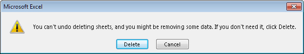
- Right-click the sheet tab and choose Move or Copy to display the Move or Copy dialog box (see Figure 14.4). Use this dialog box to specify the operation and the location for the sheet.
FIGURE 14.4 Use the Move or Copy dialog box to move or copy worksheets in the same or another workbook.
- To move a worksheet, drag the worksheet tab to the desired location. When you drag, the mouse pointer changes to a small sheet, and a small arrow guides you. To move a worksheet to a different workbook, the second workbook must be open and not maximized.
- To copy a worksheet, click the worksheet tab, and press Ctrl while dragging the tab to its desired location. When you drag, the mouse pointer changes to a small sheet with a plus sign on it. To copy a worksheet to a different workbook, the second workbook must be open and not maximized.
If you move or copy a worksheet to a workbook that already has a sheet with the same name, Excel changes the name to make it unique. For example, Sheet1 becomes Sheet1 (2). You probably want to rename the copied sheet to give it a more meaningful name (see “Changing the name of a worksheet,” earlier in this chapter).
Hiding and unhiding a worksheet
In some situations, you may want to hide one or more worksheets. Hiding a sheet may be useful if you don’t want others to see it or if you just want to get it out of the way. When a sheet is hidden, its sheet tab is also hidden. You can’t hide all the sheets in a workbook; at least one sheet must remain visible.
To hide a worksheet, right-click its sheet tab and choose Hide Sheet. The active worksheet (or selected worksheets) will be hidden from view.
To unhide a hidden worksheet, right-click any sheet tab and choose Unhide Sheet. Excel opens the Unhide dialog box, which lists all hidden sheets. Choose the sheet that you want to redisplay, and click OK. For reasons known only to a Microsoft programmer who is probably retired by now, you can’t select multiple sheets from this dialog box, so you need to repeat the command for each sheet that you want to unhide. When you unhide a sheet, it appears in its previous position among the sheet tabs.
Controlling the Worksheet View
As you add more information to a worksheet, you may find that navigating and locating what you want gets more difficult. Excel includes a few options that enable you to view your sheet, and sometimes multiple sheets, more efficiently. This section discusses a few additional worksheet options at your disposal.
Zooming in or out for a better view
Normally, everything you see on-screen is displayed at 100%. You can change the zoom percentage from 10% (very tiny) to 400% (huge). Using a small zoom percentage can help you to get a bird’s-eye view of your worksheet to see how it’s laid out. Zooming in is useful if you have trouble deciphering tiny type. Zooming doesn’t change the font size specified for the cells, so it has no effect on printed output.
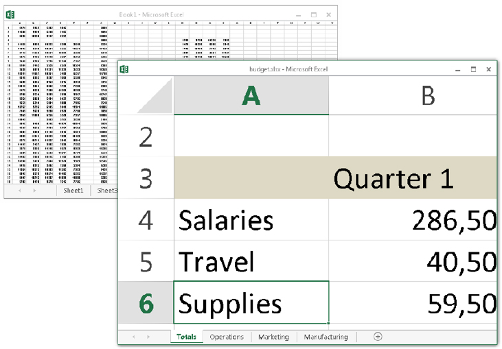
Figure 14.5 shows a window zoomed to 10% and a window zoomed to 400%.
FIGURE 14.5 You can zoom in or out for a different view of your worksheets.
You can change the zoom factor of the active worksheet window by using any of three methods:
- Use the Zoom slider located on the right side of the status bar. Drag the slider, and your screen transforms instantly.
- Press Ctrl and use the wheel button on your mouse to zoom in or out.
- Choose View ⇒ Zoom ⇒ Zoom, which displays a dialog box with some zoom options.
- Select a range of cells, and choose View ⇒ Zoom ⇒ Zoom to Selection. The selected range will be enlarged so it fills the entire window.
Viewing a worksheet in multiple windows
Sometimes, you may want to view two different parts of a worksheet simultaneously — perhaps to make referencing a distant cell in a formula easier. Or you may want to examine more than one sheet in the same workbook simultaneously. You can accomplish either of these actions by opening a new view to the workbook, using one or more additional windows.
To create and display a new view of the active workbook, choose View ⇒ Window ⇒ New Window.
Excel displays a new window for the active workbook, similar to the one shown in Figure 14.6. In this case, each window shows a different worksheet in the workbook. Notice the text in the windows’ title bars: climate data.xlsx:1 and climate data.xlsx:2. To help you keep track of the windows, Excel appends a colon and a number to each window.
FIGURE 14.6 Use multiple windows to view different sections of a workbook at the same time.
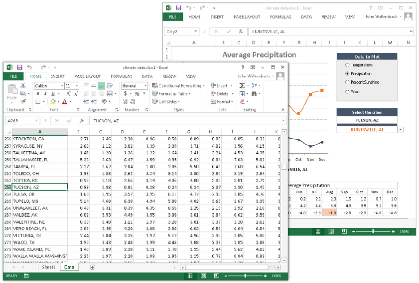
A single workbook can have as many views (that is, separate windows) as you want. Each window is independent. In other words, scrolling to a new location in one window doesn’t cause scrolling in the other window(s). However, if you make changes to the worksheet shown in a particular window, those changes are also made in all views of that worksheet.
You can close these additional windows when you no longer need them. For example, clicking the Close button on the active window’s title bar closes the active window but doesn’t close the other windows for the workbook.
Comparing sheets side by side
In some situations, you may want to compare two worksheets that are in different windows. The View Side by Side feature makes this task a bit easier.
First, make sure that the two sheets are displayed in separate windows. (The sheets can be in the same workbook or in different workbooks.) If you want to compare two sheets in the same workbook, choose View ⇒ Window ⇒ New Window to create a new window for the active workbook. Activate the first window; then choose View ⇒ Window ⇒ View Side by Side. If more than two windows are open, you see a dialog box that lets you select the window for the comparison. The two windows are tiled to fill the entire screen.
When using the Compare Side by Side feature, scrolling in one of the windows also scrolls the other window. If you don’t want this simultaneous scrolling, choose View ⇒ Window ⇒ Synchronous Scrolling (which is a toggle). If you have rearranged or moved the windows, choose View ⇒ Window ⇒ Reset Window Position to restore the windows to the initial side-by-side arrangement. To turn off the side-by-side viewing, choose View ⇒ Window ⇒ View Side by Side again.
Keep in mind that this feature is for manual comparison only. Unfortunately, Excel doesn’t provide a way to actually point out the differences between two sheets.
Splitting the worksheet window into panes
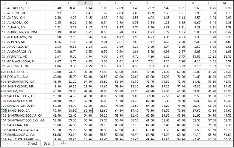
If you prefer not to clutter your screen with additional windows, Excel provides another option for viewing multiple parts of the same worksheet. Choosing View ⇒ Window ⇒ Split splits the active worksheet into two or four separate panes. The split occurs at the location of the cell pointer. If the cell pointer is in row 1 or column A, this command results in a two-pane split; otherwise, it gives you four panes. You can use the mouse to drag the individual panes to resize them.
Figure 14.7 shows a worksheet split into two panes. Notice that row numbers aren’t continuous. The top pane shows rows 8 through 20, and the bottom pane shows rows 694 through 708. In other words, splitting panes enables you to display in a single window widely separated areas of a worksheet. To remove the split panes, choose View ⇒ Window ⇒ Split again.
FIGURE 14.7 You can split the worksheet window into two or four panes to view different areas of the worksheet at the same time.
Keeping the titles in view by freezing panes
If you set up a worksheet with column headings or descriptive text in the first column, this identifying information won’t be visible when you scroll down or to the right. Excel provides a handy solution to this problem: freezing panes. Freezing panes keeps the column or row headings visible while you’re scrolling through the worksheet.
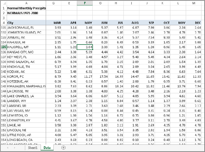
To freeze panes, start by moving the cell pointer to the cell below the row that you want to remain visible while you scroll vertically, and to the right of the column that you want to remain visible while you scroll horizontally. Then choose View ⇒ Window ⇒ Freeze Panes and select the Freeze Panes option from the drop-down list. Excel inserts dark lines to indicate the frozen rows and columns. The frozen row and column remain visible while you scroll throughout the worksheet. To remove the frozen panes, choose View ⇒ Window ⇒ Freeze Panes, and select the Unfreeze Panes option from the drop-down list.
Figure 14.8 shows a worksheet with frozen panes. In this case, rows 1:4 and column A are frozen in place. This technique allows you to scroll down and to the right to locate some information while keeping the column titles and the column A entries visible.
FIGURE 14.8 Freeze certain columns and rows to make them remain visible while you scroll the worksheet.
Most of the time, you’ll want to freeze either the first row or the first column. The View ⇒ Window ⇒ Freeze Panes drop-down list has two additional options: Freeze Top Row and Freeze First Column. Using these commands eliminates the need to position the cell pointer before freezing panes.
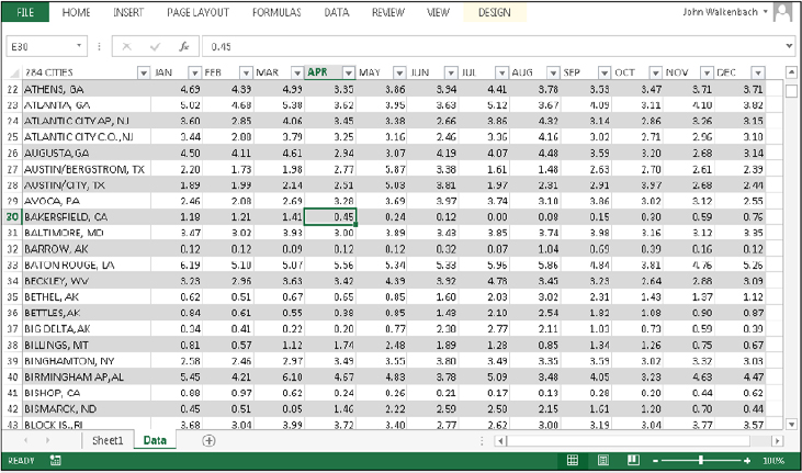
FIGURE 14.9 When using a table, scrolling down displays the table headings where the column letters normally appear.
Monitoring cells with a Watch Window
In some situations, you may want to monitor the value in a particular cell as you work. As you scroll throughout the worksheet, that cell may disappear from view. A feature known as Watch Window can help. A Watch Window displays the value of any number of cells in a handy window that’s always visible.
To display the Watch Window, choose Formulas ⇒ Formula Auditing ⇒ Watch Window. The Watch Window is actually a task pane, and you can dock it to the side of the window or drag it and make it float over the worksheet.
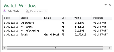
To add a cell to watch, click Add Watch and specify the cell that you want to watch. The Watch Window displays the value in that cell. You can add any number of cells to the Watch Window. Figure 14.10 shows the Watch Window monitoring four cells.
FIGURE 14.10 Use the Watch Window to monitor the value in one or more cells.
Working with Rows and Columns
This section discusses worksheet operations that involve complete rows and columns (rather than individual cells). Every worksheet has exactly 1,048,576 rows and 16,384 columns, and these values can’t be changed.
Inserting rows and columns
Although the number of rows and columns in a worksheet is fixed, you can still insert and delete rows and columns if you need to make room for additional information. These operations don’t change the number of rows or columns. Instead, inserting a new row moves down the other rows to accommodate the new row. The last row is simply removed from the worksheet if it’s empty. Inserting a new column shifts the columns to the right, and the last column is removed if it’s empty.
To insert a new row or rows, use either of these methods:
- Select an entire row or multiple rows by clicking the row numbers in the worksheet border. Right-click and choose Insert from the shortcut menu.
- Move the cell pointer to the row that you want to insert, and then choose Home ⇒ Cells ⇒ Insert ⇒ Insert Sheet Rows. If you select multiple cells in the column, Excel inserts additional rows that correspond to the number of cells selected in the column and moves the rows below the insertion down.
To insert a new column or columns, use either of these methods:
- Select an entire column by clicking its column letter in the worksheet border, also known as the column header. (Ctrl+click to select multiple adjacent columns.) Right-click and choose Insert from the shortcut menu.
- Move the cell pointer to the column that you want to insert, and then choose Home ⇒ Cells ⇒ Insert ⇒ Insert Sheet Columns. If you select multiple cells in the row, Excel inserts additional columns that correspond to the number of cells selected in the row.
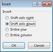
You can also insert cells, rather than just rows or columns. Select the range into which you want to add new cells and then choose Home ⇒ Cells ⇒ Insert Insert Cells (or right-click the selection and choose Insert). To insert cells, the existing cells must be shifted to the right or shifted down. Therefore, Excel displays the Insert dialog box shown in Figure 14.11 so that you can specify the direction in which you want to shift the cells. Notice that this dialog box also enables you to insert entire rows or columns.
FIGURE 14.11 You can insert partial rows or columns by using the Insert dialog box.
Deleting rows and columns
You may also want to delete rows or columns in a worksheet. For example, your sheet may contain old data that is no longer needed, or you may want to remove empty rows or columns.
To delete a row or rows, use either of these methods:
- Select an entire row or multiple rows by clicking or Ctrl+clicking the row numbers in the worksheet border (row header). Right-click and choose Delete from the shortcut menu.
- Move the cell pointer to the row that you want to delete, and then choose Home ⇒ Cells ⇒ Delete Sheet Rows. If you select multiple cells in the column, Excel deletes all rows in the selection.
Deleting columns works in a similar way. If you discover that you accidentally deleted a row or column, select Undo from the Quick Access Toolbar (or press Ctrl+Z) to undo the action.
Hiding rows and columns
In some cases, you may want to hide particular rows or columns. Hiding rows and columns may be useful if you don’t want users to see particular information, or if you need to print a report that summarizes the information in the worksheet without showing all the details.
To hide rows in your worksheet, select the row or rows that you want to hide by clicking in the row header on the left. Then right-click and choose Hide from the shortcut menu. Or you can use the commands on the Home ⇒ Cells ⇒ Format ⇒ Hide & Unhide drop-down list.
To hide columns, use the same technique, but start by selecting columns rather than rows.
A hidden row is actually a row with its height set to zero. Similarly, a hidden column has a column width of zero. When you use the navigation keys to move the cell pointer, cells in hidden rows or columns are skipped. In other words, you can’t use the navigation keys to move to a cell in a hidden row or column.
Notice, however, that Excel displays a very narrow column heading for hidden columns and a very narrow row heading for hidden rows. You can drag the column heading to make the column wider — and make it visible again. For a hidden row, drag the small row heading to make the column visible.
Another way to unhide a row or column is to choose Home ⇒ Editing ⇒ Find & Select ⇒ Go To (or its F5 equivalent) to select a cell in a hidden row or column. For example, if column A is hidden, you can press F5 and specify cell A1 (or any other cell in column A) to move the cell pointer to the hidden column. Then you can choose Home ⇒ Cells ⇒ Format ⇒ Hide & Unhide ⇒ Unhide Columns.
Changing column widths and row heights
Often, you’ll want to change the width of a column or the height of a row. For example, you can make columns narrower to show more information on a printed page. Or you may want to increase row height to create a “double-spaced” effect. Excel provides several different ways to change the widths of columns and the height of rows.
Changing column widths
Column width is measured in terms of the number of characters of a monospaced font that will fit into the cell’s width. By default, each column’s width is 8.43 units, which equates to 64 pixels (px).
Before you change the column width, you can select multiple columns so that the width will be the same for all selected columns. To select multiple columns, either drag over the column letter in the column header or Ctrl+click to select individual columns. To select all columns, click the button where the row and column headers intersect. You can change columns widths by using any of the following techniques:
- Drag the right column border with the mouse until the column is the desired width.
- Choose Home ⇒ Cells ⇒ Format ⇒ Column Width and enter a value in the Column Width dialog box.
- Choose Home ⇒ Cells ⇒ Format ⇒ AutoFit Column Width to adjust the width of the selected column so that the widest entry in the column fits. Instead of selecting an entire column, you can just select cells in the column, and the column is adjusted based on the widest entry in your selection.
- Double-click the right border of a column header to set the column width automatically to the widest entry in the column.
Changing row heights
Row height is measured in points (pt; a standard unit of measurement in the printing trade — 72 pt is equal to 1 inch). The default row height using the default font is 15 pt, or 20 px.
The default row height can vary, depending on the font defined in the Normal style. In addition, Excel automatically adjusts row heights to accommodate the tallest font in the row. So, if you change the font size of a cell to 20 pt, for example, Excel makes the row taller so that the entire text is visible.
You can set the row height manually, however, by using any of the following techniques. As with columns, you can select multiple rows.
- Drag the lower row border with the mouse until the row is the desired height.
- Choose Home ⇒ Cells ⇒ Format ⇒ Row Height and enter a value (in points) in the Row Height dialog box.
- Double-click the bottom border of a row to set the row height automatically to the tallest entry in the row. You can also choose Home ⇒ Cells ⇒ Format ⇒ Autofit Row Height for this task.
Changing the row height is useful for spacing out rows and is almost always preferable to inserting empty rows between lines of data.
Understanding Cells and Ranges
A cell is a single element in a worksheet that can hold a value, some text, or a formula. A cell is identified by its address, which consists of its column letter and row number. For example, cell D9 is the cell in the fourth column and the ninth row.
A group of cells is called a range. You designate a range address by specifying its upper-left cell address and its lower-right cell address, separated by a colon.
Here are some examples of range addresses:
| C24 | A range that consists of a single cell. |
| A1:B1 | Two cells that occupy one row and two columns. |
| A1:A100 | 100 cells in column A. |
| A1:D4 | 16 cells (four rows by four columns). |
| C1:C1048576 | An entire column of cells; this range also can be expressed as C:C. |
| A6:XFD6 | An entire row of cells; this range also can be expressed as 6:6. |
| A1:XFD1048576 | All cells in a worksheet. This range also can be expressed as either A:XFD or 1:1048576. |
Selecting ranges
To perform an operation on a range of cells in a worksheet, you must first select the range. For example, if you want to make the text bold for a range of cells, you must select the range and then choose Home ⇒ Font ⇒ Bold (or press Ctrl+B).
When you select a range, the cells appear highlighted. The exception is the active cell, which remains its normal color. Figure 14.12 shows an example of a selected range (B5:C8) in a worksheet. Cell B5, the active cell, is selected but not highlighted.
FIGURE 14.12 When you select a range, it appears highlighted, but the active cell within the range is not highlighted.
You can select a range in several ways:
- Press the left mouse button and drag, highlighting the range. Then release the mouse button. If you drag to the end of the window, the worksheet will scroll.
- Press the Shift key while you use the arrow keys to select a range.
- Press F8 and then move the cell pointer with the arrow keys to highlight the range. Press F8 again to return the navigation keys to normal movement.
- Type the cell or range address into the Name box (located to the left of the Formula bar) and press Enter. Excel selects the cell or range that you specified.
- Choose Home ⇒ Editing ⇒ Find & Select ⇒ Go To (or press F5) and enter a range’s address manually in the Go To dialog box. When you click OK, Excel selects the cells in the range that you specified.
Selecting complete rows and columns
Often, you’ll need to select an entire row or column. For example, you may want to apply the same numeric format or the same alignment options to an entire row or column. You can select entire rows and columns in much the same manner as you select ranges:
- Click the row or column header to select a single row or column.
- To select multiple adjacent rows or columns, drag over the row or column header.
- To select multiple (nonadjacent) rows or columns, press Ctrl while you click the row or column headers that you want.
- Press Ctrl+Spacebar to select a column. The column of the active cell (or columns of the selected cells) is highlighted.
- Press Shift+Spacebar to select a row. The row of the active cell (or rows of the selected cells) is highlighted.
Selecting noncontiguous ranges
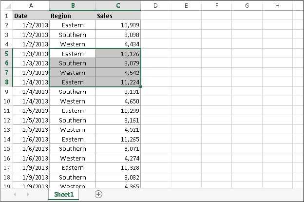
Most of the time, the ranges that you select are contiguous — a single rectangle of cells. Excel also enables you to work with noncontiguous ranges, which consist of two or more ranges (or single cells) that aren’t next to each other. Selecting noncontiguous ranges is also known as a multiple selection. If you want to apply the same formatting to cells in different areas of your worksheet, one approach is to make a multiple selection. When the appropriate cells or ranges are selected, the formatting that you select is applied to them all. Figure 14.13 shows a noncontiguous range selected in a worksheet. Three ranges are selected: A2:C3, A5:C5, and A9:C10.
FIGURE 14.13 Excel enables you to select noncontiguous ranges.
You can select a noncontiguous range in several ways:
- Select the first range (or cell). Then press and hold Ctrl as you drag the mouse to highlight additional cells or ranges.
- From the keyboard, select a range as described previously (using F8 or the Shift key). Then press Shift+F8 to select another range without canceling the previous range selections.
- Enter the range (or cell) address in the Name box and press Enter. Separate each range address with a comma.
- Choose Home ⇒ Editing ⇒ Find & Select ⇒ Go To (or press F5) to display the Go To dialog box. Enter the range (or cell) address in the Reference box, and separate each range address with a comma. Click OK, and Excel selects the ranges.
Selecting multisheet ranges
In addition to two-dimensional ranges on a single worksheet, ranges can extend across multiple worksheets to be three-dimensional ranges.
Suppose that you have a workbook set up to track budgets. A common approach is to use a separate worksheet for each department, making it easy to organize the data. You can click a sheet tab to view the information for a particular department.
Say you have a workbook with four sheets: Totals, Operations, Marketing, and Manufacturing. The sheets are laid out identically. The only difference is the values. The Totals sheet contains formulas that compute the sum of the corresponding items in the three departmental worksheets.
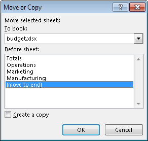
Assume that you want to apply formatting to the sheets — for example, make the column headings bold with background shading. One (albeit not-so-efficient) approach is to format the cells in each worksheet separately. A better technique is to select a multisheet range and format the cells in all the sheets simultaneously. The following is a step-by-step example of multisheet formatting, using the workbook shown in Figure 14.14.
FIGURE 14.14 In Group mode, you can work with a three-dimensional range of cells that extend across multiple worksheets.
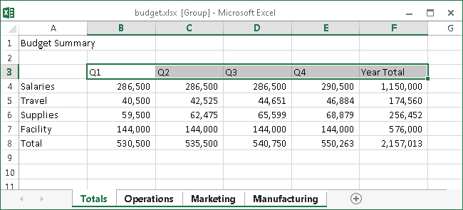
When a workbook is in Group mode, any changes that you make to cells in one worksheet also apply to the corresponding cells in all the other grouped worksheets. You can use this to your advantage when you want to set up a group of identical worksheets because any labels, data, formatting, or formulas you enter are automatically added to the same cells in all the grouped worksheets.
In general, selecting a multisheet range is a simple two-step process: Select the range in one sheet, and then select the worksheets to include in the range. To select a group of contiguous worksheets, you can press Shift and click the sheet tab of the last worksheet that you want to include in the selection. To select individual worksheets, press Ctrl and click the sheet tab of each worksheet that you want to select. If all the worksheets in a workbook aren’t laid out the same, you can skip the sheets that you don’t want to format. When you make the selection, the sheet tabs of the selected sheets display in bold with underlined text, and Excel displays [Group] in the title bar.
Selecting special types of cells
As you use Excel, you may need to locate specific types of cells in your worksheets. For example, wouldn’t it be handy to be able to locate every cell that contains a formula — or perhaps all the formula cells that depend on the active cell? Excel provides an easy way to locate these and many other special types of cells: Select a range, and choose Home ⇒ Editing ⇒ Find & Select ⇒ Go to Special to display the Go to Special dialog box, shown in Figure 14.15.
FIGURE 14.15 Use the Go to Special dialog box to select specific types of cells.
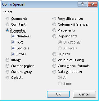
After you make your choice in the dialog box, Excel selects the qualifying subset of cells in the current selection. Often, this subset of cells is a multiple selection. If no cells qualify, Excel lets you know with the message No cells were found.
Table 14.1 offers a description of the options available in the Go to Special dialog box. Some of the options are very useful.
TABLE 14.1 Go to Special Options
| Option | What it does |
| Comments | Selects the cells that contain a cell comment. |
| Constants | Selects all nonempty cells that don’t contain formulas. Use the check boxes under the Formulas option to choose which types of nonformula cells to include. |
| Formulas | Selects cells that contain formulas. Qualify this by selecting the type of result: numbers, text, logical values (TRUE or FALSE), or errors. |
| Blanks | Selects all empty cells. If a single cell is selected when the dialog box displays, this option selects the empty cells in the used area of the worksheet. |
| Current region | Selects a rectangular range of cells around the active cell. This range is determined by surrounding blank rows and columns. You can also press Ctrl+Shift+8 (Ctrl+∗). |
| Current array | Selects the entire array. |
| Objects | Selects all embedded objects on the worksheet, including charts and graphics. |
| Row differences | Analyzes the selection and selects cells that are different from other cells in each row. |
| Column differences | Analyzes the selection and selects the cells that are different from other cells in each column. |
| Precedents | Selects cells that are referred to in the formulas in the active cell or selection (limited to the active sheet). You can select either direct precedents or precedents at any level. |
| Dependents | Selects cells with formulas that refer to the active cell or selection (limited to the active sheet). You can select either direct dependents or dependents at any level. |
| Last cell | Selects the bottom-right cell in the worksheet that contains data or formatting. For this option, the entire worksheet is examined, even if a range is selected when the dialog box displays. |
| Visible cells only | Selects only visible cells in the selection. This option is useful when dealing with a filtered list or table. |
| Conditional formats | Selects cells that have a conditional format applied (by choosing Home ⇒ Styles ⇒ Conditional Formatting). The All option selects all such cells. The Same option selects only the cells that have the same conditional formatting as the active cell. |
| Data validation | Selects cells that are set up for data entry validation (by choosing Data ⇒ Date Tools ⇒ Data Validation). The All option selects all such cells. The Same option selects only the cells that have the same validation rules as the active cell. |
Selecting cells by searching
Another way to select cells is to choose Home ⇒ Editing ⇒ Find & Select ⇒ Find (or press Ctrl+F), which allows you to select cells by their contents. Click the Options button to display additional choices for refining the search.
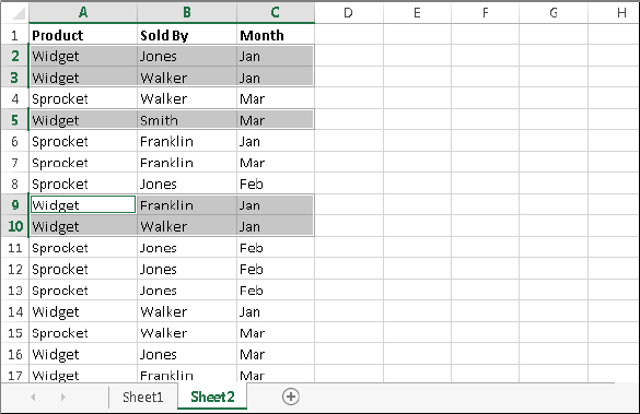
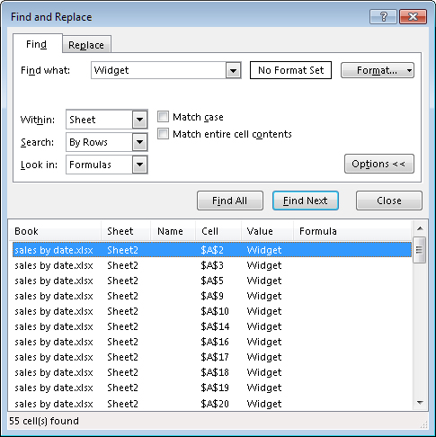
Enter the text that you’re looking for; then click Find All. The dialog box expands to display all the cells that match your search criteria. For example, Figure 14.16 shows the dialog box after Excel has located all cells that contain the text Widget. You can click an item in the list, and the screen will scroll so that you can view the cell in context. To select all the cells in the list, first select any single item in the list. Then press Ctrl+A to select them all.
FIGURE 14.16 The Find and Replace dialog box, with its results listed
The Find and Replace dialog box supports two wildcard characters:
| ? | Matches any single character |
| * | Matches any number of characters |
Wildcard characters also work with values when the Match Entire Cell Contents option is selected. For example, searching for 3* locates all cells that contain a value that begins with 3. Searching for 1?9 locates all three-digit entries that begin with 1 and end with 9. Searching for *00 locates values that end with two zeros.
~*NONE~*If your searches don’t seem to be working correctly, double-check these three options (which sometimes have a way of changing on their own):
- Match case: If this check box is selected, the case of the text must match exactly. For example, searching for smith does not locate Smith.
- Match entire cell contents: If this check box is selected, a match occurs if the cell contains only the search string (and nothing else). For example, searching for Excel doesn’t locate a cell that contains Microsoft Excel. When using wildcard characters, an exact match is not required.
- Look in: This drop-down list has three options: Values, Formulas, and Comments. If, for example, Values is selected, searching for 900 doesn’t find a cell that contains 900 if that value is generated by a formula (unless the formula itself contains 900).
Copying or Moving Ranges
As you create a worksheet, you may find it necessary to copy or move information from one location to another. Excel makes copying or moving ranges of cells easy. Here are some common things you might do:
- Copy a cell to another location.
- Copy a cell to a range of cells. The source cell is copied to every cell in the destination range.
- Copy a range to another range. Both ranges must be the same size.
- Move a range of cells to another location.
The primary difference between copying and moving a range is the effect of the operation on the source range. When you copy a range, the source range is unaffected. When you move a range, the contents are removed from the source range.
Copying or moving consists of two steps (although shortcut methods are available):
Because copying (or moving) is used so often, Excel provides many different methods. I discuss each method in the following sections. Copying and moving are similar operations, so I point out only important differences between the two.
Copying by using Ribbon commands
Choosing Home ⇒ Clipboard ⇒ Copy transfers a copy of the selected cell or range to the Windows Clipboard and the Office Clipboard. After performing the copy part of this operation, select the cell that will hold the copy and choose Home ⇒ Clipboard ⇒ Paste.
Instead of choosing Home ⇒ Clipboard ⇒ Paste, you can just activate the destination cell and press Enter. If you use this technique, Excel removes the copied information from the Clipboard so that it can’t be pasted again.
If you’re copying a range, you don’t need to select an entire same-sized range before you click the Paste button. You only need to click the upper-left cell in the destination range.
Copying by using shortcut menu commands and keyboard shortcuts
If you prefer, you can use the following shortcut menu commands for copying and pasting:
- Right-click the range and choose Copy (or Cut) from the shortcut menu to copy the selected cells to the Clipboard.
- Right-click and choose Paste from the shortcut menu that appears to paste the Clipboard contents to the selected cell or range.
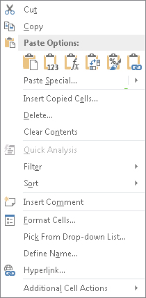
For more control over how the pasted information appears, use one of the buttons under Paste Options in the shortcut menu (see Figure 14.17).
FIGURE 14.17 The paste icons on the shortcut menu provide more control over how the pasted information appears.
Instead of using Paste, you can just activate the destination cell and press Enter. If you use this technique, Excel removes the copied information from the Clipboard so that it can’t be pasted again.
The copy and paste operations also have keyboard shortcuts (these are the same as those available in other applications):
- Ctrl+C copies the selected cells to both the Windows Clipboard and the Office Clipboard.
- Ctrl+X cuts the selected cells to both the Windows Clipboard and the Office Clipboard.
- Ctrl+V pastes the Windows Clipboard contents to the selected cell or range.
Copying or moving by using drag-and-drop
Excel also enables you to copy or move a cell or range by dragging. Unlike other methods of copying and moving, dragging and dropping does not place any information on either the Windows Clipboard or the Office Clipboard.
To copy using drag-and-drop, select the cell or range that you want to copy and then press Ctrl and move the mouse to one of the selection’s borders (the mouse pointer is augmented with a small plus sign). Then, drag the selection to its new location while you continue to press the Ctrl key. The original selection remains behind, and Excel makes a new copy when you release the mouse button.
To move a range using drag-and-drop, don’t press Ctrl while dragging the border.
Copying to adjacent cells
Often, you need to copy a cell to an adjacent cell or range. This type of copying is quite common when working with formulas. For example, if you’re working on a budget, you might create a formula to add the values in column B. You can use the same formula to add the values in the other columns. Rather than re-enter the formula, you can copy it to the adjacent cells.
Excel provides additional options for copying to adjacent cells. To use these commands, activate the cell that you’re copying and extend the cell selection to include the cells that you’re copying to. Then issue the appropriate command from the following list for one-step copying:
- Home ⇒ Editing ⇒ Fill ⇒ Down (or Ctrl+D) copies the cell to the selected range below.
- Home ⇒ Editing ⇒ Fill ⇒ Right (or Ctrl+R) copies the cell to the selected range to the right.
- Home ⇒ Editing ⇒ Fill ⇒ Up copies the cell to the selected range above.
- Home ⇒ Editing ⇒ Fill ⇒ Left copies the cell to the selected range to the left.
None of these commands places information on either the Windows Clipboard or the Office Clipboard.
Copying a range to other sheets
You can use the copy procedures described previously to copy a cell or range to another worksheet, even if the worksheet is in a different workbook. You must, of course, activate the other worksheet before you select the location to which you want to copy.
Excel offers a quicker way to copy a cell or range and paste it to other worksheets in the same workbook.
Using the Office Clipboard to paste
Whenever you cut or copy information in an Office program, such as Excel, you can place the data on both the Windows Clipboard and the Office Clipboard. When you copy information to the Office Clipboard, you append the information to the Office Clipboard instead of replacing what is already there. With multiple items stored on the Office Clipboard, you can then paste the items either individually or as a group.
To use the Office Clipboard, you first need to open it. Click the dialog box launcher on the bottom right of the Home ⇒ Clipboard group to toggle the Clipboard pane on and off.
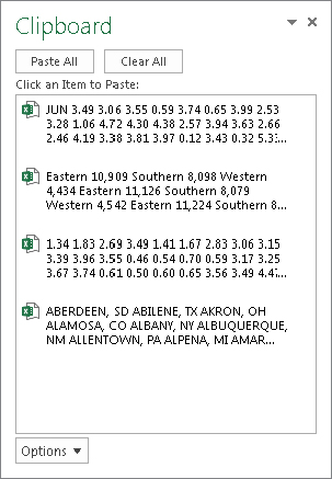
After you open the Clipboard task pane, select the first cell or range that you want to copy to the Office Clipboard and copy it by using any of the preceding techniques. Repeat this process, selecting the next cell or range that you want to copy. As soon as you copy the information, the Clipboard pane shows you the number of items that you’ve copied and a brief description (it will hold up to 24 items). Figure 14.18 shows the Office Clipboard with four copied items.
FIGURE 14.18 Use the Clipboard pane to copy and paste multiple items.
When you’re ready to paste information, select the cell into which you want to paste information. To paste an individual item, click it in the Clipboard pane. To paste all the items that you’ve copied, click the Paste All button (which is at the top of the Clipboard pane). The items are pasted, one after the other. The Paste All button is probably more useful in Word, for situations in which you copy text from various sources and then paste it all at once.
You can clear the contents of the Office Clipboard by clicking the Clear All button.
The following items about the Office Clipboard and how it functions are worth noting:
- Excel pastes the contents of the Windows Clipboard (the last item you copied to the Office Clipboard) when you paste by choosing Home ⇒ Clipboard ⇒ Paste, by pressing Ctrl+V, or by right-clicking and choosing Paste from the shortcut menu.
- The last item that you cut or copied appears on both the Office Clipboard and the Windows Clipboard.
- Pasting from the Office Clipboard also places that item on the Windows Clipboard. If you choose Paste All from the Office Clipboard toolbar, you paste all items stored on the Office Clipboard onto the Windows Clipboard as a single item.
- Clearing the Office Clipboard also clears the Windows Clipboard.
Pasting in special ways
You may not always want to copy everything from the source range to the destination range. For example, you may want to copy only the formula results rather than the formulas themselves. Or you may want to copy the number formats from one range to another without overwriting any existing data or formulas.
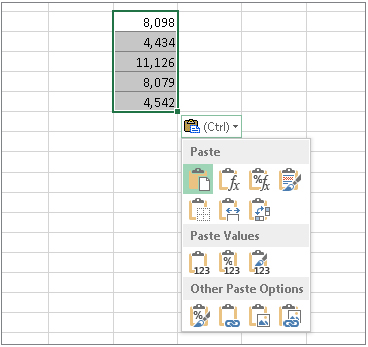
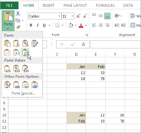
To control what is copied into the destination range, choose Home ⇒ Clipboard ⇒ Paste and use the drop-down menu shown in Figure 14.19. When you hover your mouse pointer over an icon, you’ll see a preview of the pasted information in the destination range. Click the icon to use the selected paste option.
FIGURE 14.19 Excel offers several pasting options, with preview. Here, the information is copied from D2:E5 and is being pasted beginning at cell D10 using the Transpose option.
The paste options are:
- Paste (P): Pastes the cell’s contents, formats, and data validation from the Windows Clipboard.
- Formulas (F): Pastes formulas but not formatting.
- Formulas & Number Formatting (O): Pastes formulas and number formatting only.
- Keep Source Formatting (K): Pastes formulas and all formatting.
- No Borders (B): Pastes everything except borders that appear in the source range.
- Keep Source Column Width (W): Pastes formulas and duplicates the column width of the copied cells.
- Transpose (T): Changes the orientation of the copied range. Rows become columns, and columns become rows. Any formulas in the copied range are adjusted so that they work properly when transposed.
- Merge Conditional Formatting (G): This icon is displayed only when the copied cells contain conditional formatting. When clicked, it merges the copied conditional formatting with any conditional formatting in the destination range.
- Values (V): Pastes the results of formulas. The destination for the copy can be a new range or the original range. In the latter case, Excel replaces the original formulas with their current values.
- Values & Number Formatting (A): Pastes the results of formulas plus the number formatting.
- Values & Source Formatting (E): Pastes the results of formulas plus all formatting.
- Formatting (R): Pastes only the formatting of the source range.
- Paste Link (N): Creates formulas in the destination range that refer to the cells in the copied range.
- Picture (U): Pastes the copied information as a picture.
- Linked Picture (I): Pastes the copied information as a “live” picture that is updated if the source range is changed.
- Paste Special: Displays the Paste Special dialog box (described in the next section).
Using the Paste Special dialog box
For yet another pasting method, choose Home ⇒ Clipboard ⇒ Paste ⇒ Paste Special to display the Paste Special dialog box (see Figure 14.20). You can also right-click and choose Paste Special from the shortcut menu to display this dialog box. This dialog box has several options, explained next.
FIGURE 14.20 The Paste Special dialog box

- All: Pastes the cell’s contents, formats, and data validation from the Windows Clipboard
- Formulas: Pastes values and formulas, with no formatting
- Values: Pastes values and the results of formulas (no formatting). The destination for the copy can be a new range or the original range. In the latter case, Excel replaces the original formulas with their current values.
- Formats: Copies only the formatting
- Comments: Copies only the cell comments from a cell or range. This option doesn’t copy cell contents or formatting.
- Validation: Copies the validation criteria so the same data validation will apply. Data validation is applied by choosing Data ⇒ Data Tools ⇒ Data Validation.
- All Using Source Theme: Pastes everything, but uses the formatting from the document theme of the source. This option is relevant only if you’re pasting information from a different workbook, and the workbook uses a different document theme than the active workbook.
- All Except Borders: Pastes everything except borders that appear in the source range
- Column Widths: Pastes only column width information
- Formulas and Number Formats: Pastes all values, formulas, and number formats (but no other formatting)
- Values and Number Formats: Pastes all values and numeric formats but not the formulas themselves
- All merging conditional formats: Merges the copied conditional formatting with any conditional formatting in the destination range. This option is enabled only when you’re copying a range that contains conditional formatting.
In addition, the Paste Special dialog box enables you to perform other operations, described in the following sections.
Performing mathematical operations without formulas
The option buttons in the Operation section of the Paste Special dialog box let you perform an arithmetic operation on values and formulas in the destination range. For example, you can copy a range to another range and select the Multiply operation. Excel multiplies the corresponding values in the source range and the destination range and replaces the destination range with the new values.
This feature also works with a single copied cell, pasted to a multi-cell range. Assume that you have a range of values, and you want to increase each value by 5 percent. Enter 105% into any blank cell and copy that cell to the Clipboard. Then select the range of values and bring up the Paste Special dialog box. Select the Multiply option, and each value in the range is multiplied by 105%.
Skipping blanks when pasting
The Skip Blanks option in the Paste Special dialog box prevents Excel from overwriting cell contents in your paste area with blank cells from the copied range. This option is useful if you’re copying a range to another area but don’t want the blank cells in the copied range to overwrite existing data.
Transposing a range
The Transpose option in the Paste Special dialog box changes the orientation of the copied range. Rows become columns, and columns become rows. Any formulas in the copied range are adjusted so that they work properly when transposed. Note that you can use this check box with the other options in the Paste Special dialog box.
Using Names to Work with Ranges
Dealing with cryptic cell and range addresses can sometimes be confusing, especially when you deal with formulas, which are covered in Chapter 15. Fortunately, Excel allows you to assign descriptive names to cells and ranges. For example, you can give a cell a name such as Interest_Rate, or you can name a range JulySales. Working with these names (rather than cell or range addresses) has several advantages:
- A meaningful range name (such as Total_Income) is much easier to remember than a cell address (such as AC21).
- Entering a name is less error prone than entering a cell or range address, and if you type a name incorrectly in a formula, Excel will display a #NAME? error.
- You can quickly move to areas of your worksheet either by using the Name box, located at the left side of the Formula bar (click the arrow to drop down a list of defined names) or by choosing Home ⇒ Editing ⇒ Find & Select ⇒ Go To (or pressing F5) and specifying the range name.
- Creating formulas is easier. You can paste a cell or range name into a formula by using Formula AutoComplete, another feature covered in Chapter 15.
- Names make your formulas more understandable and easier to use. A formula such as =Income—Taxes is more intuitive than =D20—D40.
Creating range names in your workbooks
Excel provides several different methods that you can use to create range names. Before you begin, however, you should be aware of a few rules:
- Names can’t contain any spaces. You may want to use an underscore character to simulate a space (such as Annual_Total).
- You can use any combination of letters and numbers, but the name must begin with a letter, underscore, or backslash. A name can’t begin with a number (such as 3rdQuarter) or look like a cell address (such as QTR3). If these are desirable names, though, you can precede the name with an underscore or a backslash: for example, _3rd Quarter and QTR3.
- Symbols — except for underscores, backslashes, and periods — aren’t allowed.
- Names are limited to 255 characters, but it’s a good practice to keep names as short as possible, but still meaningful.
Using the Name box
The fastest way to create a name is to use the Name box (to the left of the Formula bar). Select the cell or range to name, click the Name box, and type the name. Press Enter to create the name. (You must press Enter to actually record the name; if you type a name and then click in the worksheet, Excel doesn’t create the name.)
If you type an invalid name (such as May21, which is a cell address), Excel activates that address (and doesn’t warn you that the name is not valid). If the name you type includes an invalid character, Excel displays an error message. If a name already exists, you can’t use the Name box to change the range to which that name refers. Attempting to do so simply selects the range.
The Name box is a drop-down list and shows all names in the workbook. To choose a named cell or range, click the Name box and choose the name. The name appears in the Name box, and Excel selects the named cell or range in the worksheet.
Using the New Name dialog box
For more control over naming cells and ranges, use the New Name dialog box. Start by selecting the cell or range that you want to name. Then choose Formulas ⇒ Defined Names ⇒ Define Name. Excel displays the New Name dialog box, shown in Figure 14.21. Note that this is a resizable dialog box. Drag a border to change the dimensions.
FIGURE 14.21 Create names for cells or ranges by using the New Name dialog box.
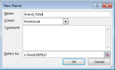
Type a name in the Name text field (or use the name that Excel proposes, if any). The selected cell or range address appears in the Refers To text field. Use the Scope drop-down list to indicate the scope for the name. The scope indicates where the name will be valid, and it’s either the entire workbook or a particular sheet. If you like, you can add a comment that describes the named range or cell. Click OK to add the name to your workbook and close the dialog box.
Using the Create Names from Selection dialog box
You may have a worksheet that contains text that you want to use for names for adjacent cells or ranges. For example, you may want to use the text in column A to create names for the corresponding values in column B. Excel makes this task easy.
To create names by using adjacent text, start by selecting the name text and the cells that you want to name. (These items can be individual cells or ranges of cells.) The names must be adjacent to the cells that you’re naming. (A multiple selection is allowed.) Then choose Formulas ⇒ Defined Names ⇒ Create from Selection. Excel displays the Create Names from Selection dialog box, shown in Figure 14.22.
FIGURE 14.22 Use the Create Names from Selection dialog box to name cells using labels that appear in the worksheet.
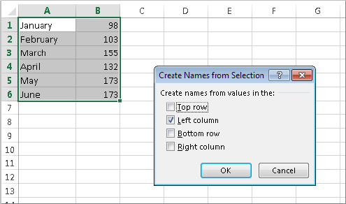
The check marks in the Create Names from Selection dialog box are based on Excel’s analysis of the selected range. For example, if Excel finds text in the first row of the selection, it proposes that you create names based on the top row. If Excel didn’t guess correctly, you can change the check boxes. Click OK, and Excel creates the names. Using the data in Figure 14.22, Excel creates six names: January for cell B1, February for cell B2, and so on.
Managing names
A workbook can have any number of named cells and ranges. If you have many names, you should know about the Name Manager, shown in Figure 14.23.
FIGURE 14.23 Use the Name Manager to work with range names.
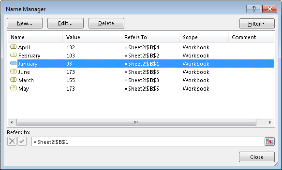
The Name Manager appears when you choose Formulas ⇒ Defined Names ⇒ Name Manager (or press Ctrl+F3). The Name Manager has the following features:
- Displays information about each name in the workbook: You can resize the Name Manager dialog box, widen the columns to show more information, and even rearrange the order of the columns. You can also click a column heading to sort the information by the column.
- Allows you to filter the displayed names: Clicking the Filter button lets you show only those names that meet a certain criteria. For example, you can view only the worksheet-level names.
- Provides quick access to the New Name dialog box: Click the New button to create a new name without closing the Name Manager.
- Lets you edit names: To edit a name, select it in the list and then click the Edit button. You can change the name itself, modify the Refers to range, or edit the comment.
- Lets you quickly delete unneeded names: To delete a name, select it in the list and click Delete.
If you delete the rows or columns that contain named cells or ranges, the names contain an invalid reference. For example, if cell A1 on Sheet1 is named Interest and you delete row 1 or column A, the name Interest then refers to =Sheet1!#REF! (that is, to an erroneous reference). If you use Interest in a formula, the formula displays #REF.
Adding Comments to Cells
Documentation that explains certain elements in the worksheet can often be helpful. One way to document your work is to add comments to cells. This feature is useful when you need to describe a particular value or explain how a formula works.
To add a comment to a cell, select the cell and use any of these actions:
- Choose Review ⇒ Comments ⇒ New Comment.
- Right-click the cell and choose Insert Comment from the shortcut menu.
- Press Shift+F2.
Excel inserts a comment that points to the active cell. Initially, the comment consists of your name, as specified in the General tab of the Excel Options dialog box (choose File ⇒ Options to display this dialog box). You can delete your name from the comment, if you like. Enter the text for the cell comment and then click anywhere in the worksheet to hide the comment. You can change the size of the comment by clicking and dragging any of its borders. Figure 14.24 shows a cell with a comment.
FIGURE 14.24 You can add comments to cells to help point out specific items in your worksheets.
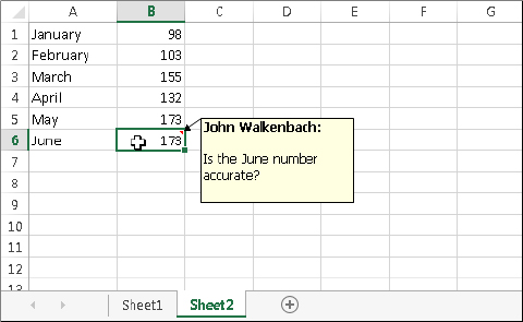
Cells that have a comment display a small red triangle in the upper-right corner. When you move the mouse pointer over a cell that contains a comment (or activate the cell), the comment becomes visible.
You can force a comment to be displayed even when its cell is not activated. Right-click the cell and choose Show/Hide Comments. Although this command refers to “comments” (plural), it affects only the comment in the active cell. To return to normal (make the comment appear only when its cell is activated or the mouse point hovers over it), right-click the cell and choose Hide Comment.
Formatting comments
If you don’t like the default look of cell comments, you can make some changes. Right-click the cell and choose Edit Comment. Select the text in the comment and use the commands of the Font and the Alignment groups (on the Home tab) to make changes to the comment’s appearance.
For even more formatting options, right-click the comment’s border and choose Format Comment from the shortcut menu. Excel responds by displaying the Format Comment dialog box, which allows you to change many aspects of its appearance, including color, border, and margins.
You can also display an image inside a comment. Right-click the cell and choose Edit Comment. Then right-click the comment’s border and choose Format Comment. Select the Colors and Lines tab in the Format Comment dialog box. Click the Color drop-down list and select Fill Effects. In the Fill Effects dialog box, click the Picture tab and then click the Select Picture button to specify a graphics file. Figure 14.25 shows a comment that contains a picture.
FIGURE 14.25 This comment contains a graphics image.

Working further with comments
Comments are there to present information, and you need to know how to read and display comments. Here are additional key actions you’ll perform with comments:
- Reading comments: To read all comments in a workbook, choose Review ⇒ Comments ⇒ Next. Keep clicking Next to cycle through all the comments in a workbook. Choose Review ⇒ Comments ⇒ Previous to view the comments in reverse order.
NoteYou can also access the Page Setup box from the Print panel of Backstage view.
- Hiding and showing comments: If you want all cell comments to be visible (regardless of the location of the cell pointer), choose Review ⇒ Comments ⇒ Show All Comments. This command is a toggle; select it again to hide all cell comments. To toggle the display of an individual comment, select its cell, and then choose Review ⇒ Comments ⇒ Show/Hide Comment.
- Selecting comments: To quickly select all cells in a worksheet that contain a comment, choose Home ⇒ Editing ⇒ Find & Select ⇒ Go to Special. Then choose the Comments option and click OK.
- Editing comments: To edit a comment, activate the cell, right-click, and then choose Edit Comment from the shortcut menu. Or select the cell and press Shift+F2. After you make your changes, click any cell.
- Deleting comments: To delete a cell comment, activate the cell that contains the comment and then choose Review ⇒ Comments ⇒ Delete. Or right-click and then choose Delete Comment from the shortcut menu.
- Printing comments: Comments do not print by default. Click the dialog box launcher in the Page Layout ⇒ Page Setup group. In the Page Setup dialog box, click the Sheet tab. Make your choice from the Comments drop-down control: At End of Sheet or As Displayed on Sheet. Click OK to close the Page Setup dialog box or click the Print button to print the worksheet.
Summary
This chapter taught essential skills dealing with worksheets, cells, and ranges. You should now be equipped with a wide variety of skills, including the ability to:
- Create, copy, move, and rename worksheets.
- Change worksheet zoom.
- Resize, insert, and delete rows and columns.
- Hide and redisplay rows and columns.
- Use various techniques to select cells and ranges.
- Perform standard and special copy and paste operations.
- Name ranges and work with range names.
- Add and change cell comments.