
307
18
BelievableDeadReckoning
forNetworkedGames
Curtiss Murphy
Alion Science and Technology
18.1Introduction
Your team’s producer decides that it’s time to release a networked game, saying
“We can publish across a network, right?” Bob kicks off a few internet searches
and replies, “Doesn’t look that hard.” He dives into the code, and before long,
Bob is ready to begin testing. Then, he stares in bewilderment as the characters
jerk and warp across the screen and the vehicles hop, bounce, and sink into the
ground. Thus begins the nightmare that will be the next few months of Bob’s life,
as he attempts to implement dead reckoning “just one more tweak” at a time.
This gem describes everything needed to add believable, stable, and efficient
dead reckoning to a networked game. It covers the fundamental theory, compares
algorithms, and makes a case for a new technique. It explains what’s tricky about
dead reckoning, addresses common myths, and provides a clear implementation
path. The topics are demonstrated with a working networked game that includes
source code. This gem will help you avoid countless struggles and dead ends so
that you don’t end up like Bob.
18.2Fundamentals
Bob isn’t a bad developer; he just made some reasonable, but misguided, as-
sumptions. After all, the basic concept is pretty straight forward. Dead reckoning
is the process of predicting where an actor is right now by using its last known
position, velocity, and acceleration. It applies to almost any type of moving actor,
including cars, missiles, monsters, helicopters, and characters on foot. For each

308
remote
a
dates a
b
orientati
position
next up
d
Bob is r
i
a differe
Myth
Let’s
s
netwo
r
knowl
e
exact
s
packet
percei
v
perfec
t
Basic
M
To deri
v
network
.
first kin
e
straight
f
the valu
e
it at ve
l
reckone
d
a
cto
r
b
eing
c
b
out its kine
m
on, and angu
l
we received
d
ate, we do
s
i
ght that the
fu
n
t story.
Busting—
G
s
tart with the
r
ked enviro
n
e
dge of the s
s
tate of all re
m
loss, zero l
a
v
ed
t
ruth. Th
u
t
re-creation.
M
ath
v
e the math,
w
.
In this case,
e
matic state
u
f
orward linea
r
e
s from the
m
l
ocity
0
V
wi
t
d
position
t
Q
1
c
ontrolled so
m
m
atic state t
h
l
ar velocity.
I
on the netw
o
s
ome sort of
fu
ndamentals
G
roundTr
u
following fa
c
n
ment. “Gro
u
tate of all ac
m
ote actors
w
a
tency envir
o
u
s, the goal
b
w
e start with
t
one of our o
p
u
pdate as it c
a
r
physics pr
o
m
essage, we
p
t
h accelerati
o
at a specific
t
t
Q
P
Figure 18.1
.
8.Believabl
e
m
ewhere els
e
h
at include i
t
I
n the simple
s
o
rk and proje
c
blending an
d
aren’t that c
o
u
th
c
t: there is n
o
u
nd truth”
i
tors at all ti
m
w
ithout sendi
n
o
nment. Wha
t
b
ecomes beli
e
t
he simplest
c
p
ponents is
d
a
me into vie
w
o
ble
m
, as de
s
p
ut the vehicl
e
o
n
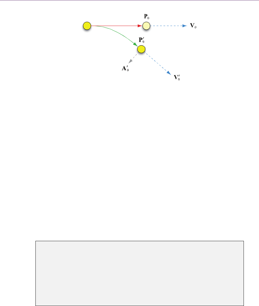
0
A
, as s
h
t
ime T is calc
00
1
2
T
P
V
A
.
The first upd
a
e
DeadReck
o
e
on the net
w
t
s position,
v
s
t implement
a
c
t it forward
d
start the p
r
o
mplex, but
m
o
such thing
a
i
mplies that
m
es. Surely,
y
n
g updates e
v
t
you have i
n
e
vable estim
a
c
ase: a new a
c
d
riving a tank
w
. From he
r
e
s
cribed by A
r
e at position
h
own in Fi
g
c
ulated with t
h
2
0
T
A
.
a
te is simple.
o
ningforNet
w
w
ork, we rec
v
elocity, acc
e
a
tion, we tak
e
in time. The
n
r
ocess all ov
e
m
aking it beli
e
a
s ground tr
u
you have
p
y
ou can’t kn
o
v
ery frame in
n
stead is yo
u
a
tion, as opp
o
ctor comes a
c
, and we rec
e
e
, dead recko
n
r
onson [199
7
0
P
and begi
n
g
ure 18.1. T
h
h
e equation
w
orkedGam
e
eive up-
e
lera
t
ion,
e
the last
n
, on the
e
r again.
e
vable is
u
th in a
p
erfect
o
w the
a zero
u
r own
o
sed to
c
ross the
e
ived our
n
ing is a
7
]. Using
n
moving
h
e dead-
e
s
18.2Fundamenta
Fi
gu
the
g
C
har
d
poi
n
gue
s
actu
a
the
l
nig
h
(e.g.
T
whe
r
ture
.
Inst
e
b
e i
n
M
T
h
i
m
pa
s
di
s
w
r
sh
i
ls
u
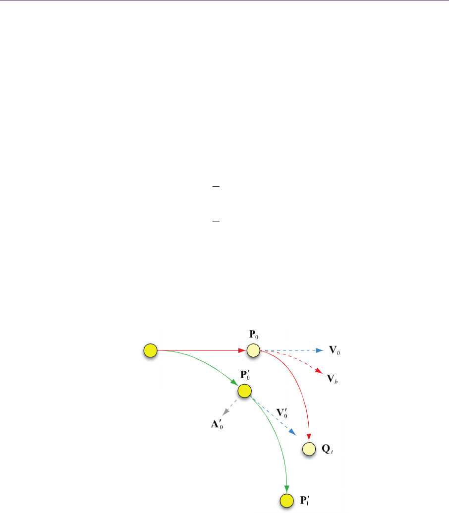
re 18.2. The
n
g
reen curve is t
h
C
ontinuing
o
d
right. Soon
n
t, we have c
o
s
sed he woul
d
a
lly went, o
u
l
ast thing we
h
tmares. Sinc
e
,
0
P
) to indic
a
T
o resolve t
h
r
e we thoug
h
.
Don’t both
e
e
ad, just mov
e
n
the future,
P
ythBustin
g
h
e human bra
i
m
portantly, ch
a
s
t our periph
e
s
continuities
i
r
ong location
.
i
mmies are t
h
n
ext update cre
h
e actual path.
o
ur scenario,
, we receive
o
nflicting re
a
d
be using th
e
u
r new
0
P
, w
h
know to be
e
there are t
w
a
te the last k
n
h
e two realit
i
h
t the tank w
o
e
r to path th
e
e
it from wh
e
1
P
.
g
—Discont
i
i
n is amazin
g
a
nges in patt
e
e
ral vision.
W
i
n a vehicle
p
.
Therefore,
d
h
e enemy.
ates two realit
i
the opponen
t
a message
u
a
lities. The fi
r
e
previous fo
h
ich we refer
correct. Thi
s
w
o versions o
f
n
own, as sho
w
i
es, we need
o
uld be, and
w
e
remote tan
k
e
re it is now,
P
i
nuitiesAr
e
g
at recognizi
n
e
rns, such as
w
W
hat this me
a
p
ath long be
f
d
iscontinuitie
i
es. The red li
n
t
saw us, slo
w
updating his
r
st reality is
t
o
rmula. The s
to as the las
t
s
dual state i
s
f
each value,
w
w
n in Figure
to create a
b
w
here we est
k
through its
0
P
, to where
w
e
NotMin
o
ng patterns [
K
when the tin
i
a
ns is that pl
f
ore they real
s such as ho
p
n
e is the estim
a
w
ed his tan
k
kinematic s
t
he position
Q
econd realit
y
t
known state
s
the beginn
i
w
e use the p
r
18.2.
b
elievable c
u
imate it will
last known
p
w
e think it is
o
r
K
oste
r
2005]
i
est piece of
f
l
ayers will n
o
ize the vehic
p
s, warps, w
o
a
ted path, and
k
, and took a
tate. At this
t
Q
where we
y
is where he
because i
t
’s
i
ng of Bob’s
r
ime notation
u
rve between
be in the fu-
p
osition,
0
P
.
supposed to
and, more
f
uzz moves
o
tice subtle
le is in the
o
bbles, and
309

310 18.BelievableDeadReckoningforNetworkedGames
18.3PickanAlgorithm,AnyAlgorithm
If you crack open any good 3D math textbook, you’ll find a variety of algorithms
for defining a curve. Fortunately, we can discard most of them right away be-
cause they are too CPU intensive or are not appropriate (e.g., B-splines do not
pass through the control points). For dead reckoning, we have the additional re-
quirement that the algorithm must work well for a single segment of a curve
passing through two points: our current location
0
P
and the estimated future loca-
tion
1
P
. Given all these requirements, we can narrow the selection down to a few
types of curves: cubic Bézier splines, Catmull-Rom splines, and Hermite curves
[Lengyel 2004, Van Verth and Bishop 2008].
These curves perform pretty well and follow smooth, continuous paths.
However, they also tend to create minor repetitive oscillations. The oscillations
are relatively small, but noticeable, especially when the actor is making a lot of
changes (e.g., moving in a circle). In addition, the oscillations tend to become
worse when running at inconsistent frame rates or when network updates don’t
come at regular intervals. In short, they are too wiggly.
ProjectiveVelocityBlending
Let’s try a different approach. Our basic problem is that we need to resolve two
realities (the current
0
P
and the last known
0
P
). Instead of creating a spline seg-
ment, let’s try a straightforward blend. We create two projections, one with the
current and one with the last known kinematic state. Then, we simply blend the
two together using a standard linear interpolation (lerp). The first attempt looks
like this:
2
00 0
1
2
ttt
TT
PPV A
(projecting from where we were),
2
00 0
1
2
ttt
TT
PPV A
(projecting from last known),
ˆ
tt tt
T
Q
PPP
(combined).
This gives
t
Q
, the dead-reckoned location at a specified time. (Time values
such as
t
T
and
ˆ
T
are explained in Section 18.4.) Note that both projection equa-
tions above use the last known value of acceleration
0
A
. In theory, the current
projection
t
P
should use the previous acceleration
0
A
to maintain
2
C
continuity.
However, in practice,
0
A
converges to the true path much quicker and reduces
oscillation.
18.3PickanAlgo
r
T
b
et
w
than
tech
n
Ma
y
let’s
twe
e
velo
T
An
d
r
ithm,AnyAl
g
T
his techniq
u
w
een our poi
n
the spline t
e
n
iques, the
o
y
be if we do
s
try it again,
e
n the old ve
l
city
b
V
. The
n
T
he techniqu
e
the red lines
Figure 18.3.
g
orithm
u
e actually w
o
n
ts. Unfortun
a
e
chniques.
U
o
scillations a
r
s
omething w
i
with a twea
k
ocity
0
V
and
n
, we use this
e
,
p
rojective
v
0
b
VV
V
0
tb
T
PPV
00
t
T
PPV
tt
QP
in Figure 18
.
Dead reckoni
n
o
rks pretty
w
a
tely, it has
o
U
pon inspecti
o
r
e caused by
i
th the veloci
t
k
. This time,
the last kno
w
to project fo
r
v
elocity blen
d
00
ˆ
T
V
V
2
0
1
2
tt
T
T
A
2
0
1
2
tt
T
T
A
ˆ
tt
T
PP
.
3 show what
n
g with projec
t
w
ell. It is sim
p
o
scillations t
h
o
n, it turns
o
the changes
ty, we can r
e
we compute
w
n velocity
V
r
ward from
w
d
ing, works l
i
(velocity
(projecti
n
(projecti
n
(combin
e
t
it looks like
tive velocity
b
p
le and gives
h
at are as ba
d
o
ut that with
in velocity
(
e
duce the osc
i
a linear inte
r
0
V
to create a
n
w
here we wer
e
i
ke this:
blending),
n
g from wher
n
g from last
k
e
d).
in action.
b
lending show
n
a nice curve
d
as or worse
all of these
(
0
V
and
0
V
).
i
llations. So,
r
polation be-
n
ew blended
e
.
e we were),
k
nown),
n
in red.
311
..................Content has been hidden....................
You can't read the all page of ebook, please click here login for view all page.