
Length Traceability Using Interferometry
Han Haitjema, Mitutoyo Research Centre Europe
This chapter presents the field of static length measurement. Some basic optics are introduced to lead up to the field of interferometry – length measurement using light. Different configurations of interferometer are presented including the Michelson, Twyman-Green, Fizeau, Jamin, Mach-Zehnder and Fabry-Pérot. Gauge blocks as length standards are discussed in detail along with gauge block interferometry. The various sources of error in gauge block interferometry are presented and the chapter finishes with some alternative methods for gauge block measurement, such as double-sided interferometry.
Keywords
Gauge Blocks; Length Bars; Interferometry; Coherence; Michelson Interferometer; Twyman-Green Interferometer; Fizeau Interferometer; Jamin Interferometer; Mach-Zehnder Interferometer; Fabry-Pérot Interferometer; Gauge Block Interferometry; Phase Correction; Aperture Correction; Fringe Fractions; Method of Exact Fractions
4.1 Traceability in length
A short historical overview of length measurement was given in Chapter 2. This chapter will take one small branch of length measurement, that of static length standards, and discuss in detail how the most accurate length measurements are made on macro-scale length standards using the technique of interferometry. These macro-scale length standards and the specialist equipment used for their measurement may not appear, at first sight, to have much relevance to micro- and nanotechnology (MNT). However, macro-scale length standards are measured to nanometre uncertainties, and many of the concepts discussed in this chapter will have relevance in later chapters. For example, much of the information here that relates to static surface-based interferometry will be developed further or modified in Chapter 5, which discusses the development of displacement interferometry.
It is also important to discuss traditional macro-scale length standards, both specification standards and physical standards, because the subject of this book is engineering nanometrology. In other words, this book is concerned with the tools, theory and practical application of nanometrology in an engineering context, rather than as an academic study. It is anticipated that the development of standards for engineering nanometrology will very much follow the route taken for macro-scale engineering in that problems concerning the interoperability of devices, interconnections, tolerancing and standardisation will lead to the requirement for testing and calibration, and this in turn will lead to the writing of specification standards and the preparation of nanoscale physical standards and the metrology tools with which to calibrate them. It may well be that an MNT version of the ISO Geometrical Product Specification (GPS) matrix [1] will evolve to serve the needs for dimensional metrology at these small scales. A discussion on this subject is presented in Ref. [2].
There is a large range of macro-scale length standards and length measuring instruments that are used throughout engineering, for example simple rulers, callipers, gauge blocks, setting rods, micrometres, step gauges, coordinate measuring machines, line scales, ring and plug gauges, verniers, stage micrometres, depth gauges, ball bars, laser trackers, ball plates, thread gauges, angle blocks and autocollimators; the list is quite extensive [3]. For any of these standards or equipment to be of any practical application to engineers, end users or metrologists, the measurements have to be traceable. Chapter 2 explained the concept of traceability and described the comparison chain for some quantities. In this chapter, we will examine in detail the traceable measurement of some of the length standards with the most basic concepts known as gauge blocks and, in doing so, we will show many of the basic principles of interferometry – perhaps the most directly traceable measurement technique for length metrology.
4.2 Gauge blocks – both a practical and traceable artefact
As discussed in Section 2.3, the end standard is one of the basic forms of material length artefact (a line standard being the alternative form of artefact). It is not only the basic form of an end standard that makes them so popular, but also the fact that Johannsson greatly enhanced the practical usability of end standards by defining gauge block sizes so that they could be used in sets and be combined to give any length with micrometre accuracy [3,4]. For these reasons, the end standard found its way from the National Measurement Institutes (NMIs) through to the shop floor.
In summary, the combination of direct traceability to the level of primary standards, the flexibility of combining them to produce any length with a minimal loss of accuracy, their availability in a range of accuracy classes and materials and the standardisation of sizes and accuracies make end standards widespread, and their traceability well established and respected.
The most commonly used gauge blocks have a standardised cross section of 9 mm×35 mm for a nominal length ln>10 mm and 9 mm×30 mm for nominal length 0.5 mm<ln<10 mm. The flatness of the surfaces (less than 0.1 μm) is such that gauge blocks can be wrung on top of each other without causing a significant additional uncertainty in length.1 This is due to the definition of a gauge block, which states that the length is defined as the distance from the measurement (reference) point on the top surface to the plane of a platen (a flat plate) adjacent to the wrung gauge block [5]. This platen should be manufactured from the same material as the gauge block and have the same surface properties (surface roughness and refractive index). Figure 4.1 is a schema, and Figure 4.2 is a photograph, of a gauge block wrung to a platen.


The definition of the length of a gauge block enables the possibility of relating the length to optical wavelengths by interferometry. Also, there is no additional uncertainty due to the wringing as the auxiliary platen could be replaced by another gauge block, where the wringing would have the same effect as the wringing to the platen, which is included in the length definition [6]. Gauge blocks are classified into accuracy classes. The less accurate classes are intended to be used in the workshop. Using mechanical comparators, these gauge blocks can be compared to reference gauge blocks that are related to wavelengths using gauge block interferometers.
Table 4.1 gives the tolerances for gauge block classes K, 0, 1 and 2 according to ISO 3650 [5]. For those to be calibrated by interferometry (class K), the absolute length is not so critical as this length is explicitly measured. However, the demands on parallelism needed for good wringing, and an accurate length definition, are highest. ISO 3650 gives the basis of demands, tolerances and definitions related to gauge blocks.
Table 4.1
Gauge Block Classes According to ISO 3650 [5]
| Class | Tolerance on Length, L | Tolerance on Parallelism for Length, L |
| K | 0.20 μm+4×10⁻⁶ L | 0.05 μm+2×10⁻⁷ L |
| 0 | 0.12 μm+2×10⁻⁶ L | 0.10 μm+3×10⁻⁷ L |
| 1 | 0.20 μm+4×10⁻⁶ L | 0.16 μm+5×10⁻⁷ L |
| 2 | 0.45 μm+8×10⁻⁶ L | 0.30 μm+7×10⁻⁷ L |
The stability of gauge blocks has been a subject of study that necessarily spans many years (see, for example Ref. [7]). In general, properly produced gauge blocks may shrink or grow 5–10 nm a year maximum, although the standard [5] allows for more than these values.
The method of gauge block calibration by interferometry is a basic example of how the bridge between the metre definition by wavelength and a material reference artefact can be made. It will be the main subject of the rest of this chapter.
4.3 Introduction to interferometry
4.3.1 Light as a wave
This chapter will introduce the aspects of optics that are required to understand interferometry. For a more thorough treatment of optics, the reader is referred to Ref. [8].
For the treatment of light, we will restrict ourselves to electromagnetic waves of optical frequencies, usually called ‘visible light’. From Maxwell’s equations, it follows that the electric field of a plane wave, with speed, c, frequency, f, and wavelength, λ, travelling in the z-direction, is given by
(4.1)
where ω=2πf=2πc/λ is the circular frequency and k is the circular wave number, k=2π/λ.
Here we use the convention that a measurable quantity, for example the amplitude, Ex, can be obtained by taking the real part of Eq. (4.1) and we assume that Ey=0, that is the light is linearly polarised in the x-direction. At the location z=0, the electric field E=Ex cos ωt. This means that the momentary electric field oscillates with a frequency f. For visible light, for example green light (λ=500 nm), this gives, with the speed of light defined as c=299 792 458 m·s−1, a frequency of f=6×10¹⁴ Hz. No electric circuit can directly follow such a high frequency; therefore, light properties are generally measured by averaging the cosine function over time. The intensity is given by the square of the amplitude, thus
(4.2)
A distortion at t=0, z=0, for example of the amplitude Ex in Eq. (4.1), will be the same as at time, t, at location z=ωt/k=ct, so the propagation velocity is c indeed.
In Eq. (4.1), the amplitudes Ex and Ey can both be complex. In that general case, we speak of elliptical polarisation; the E-vector describes an ellipse in space. If Ex and Ey are both real, the light is called linearly polarised. Another special case is when Ey=iEx, in which case the vector describes a circle in space; for that reason this case is called circular polarisation.
When light beams from different sources, or from the same source but via different paths, act on the same location, their electric fields can be added. This is called the principle of superposition and causes interference. Visible, stable interference can appear when the wavelengths are the same and there is a determined phase relationship between the superimposed waves. If the wavelengths are not the same, or the phase relationship is not constant, the effect is called beating, which means that the intensity may vary with a certain frequency.
A fixed phase relationship can be achieved by splitting light, coming from one source, into two beams and recombining the light again. An instrument that accomplishes this is called an interferometer. An example of an interferometer is shown in Figure 4.3.
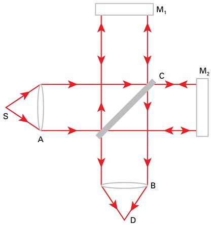
Consider the fields E1(t) and E2(t) in the interferometer in Figure 4.3, which travel paths to and from M1 and M2, respectively and combine at the detector, D. According to the principle of superposition, we can write
(4.3)
Combining Eqs. (4.1)–(4.3), with some additional assumptions, gives finally
(4.4)
where ΔL is the path difference between the two beams and I are intensities, that is the squares of the amplitudes.
Equation (4.4) is the essential equation of interference. Depending on the term 4πΔL/λ, the resultant intensity on a detector can have a minimum or a maximum, and it depends with a (co)sine function on the path difference or the wavelength.
From Eq. (4.4), it is evident that the intensity has maxima for 4pΔL/λ=2pπ, with p=0, ±1, ±2, …, so that ΔL=pλ/2 and minima for ΔL=(p+0.5)λ/2.
4.3.2 Beat measurement when ω1 ≠ ω2
If either E1 or E2 is shifted in frequency, or if E1 and E2 originate from sources with a different frequency, we can write analogous to Eq. (4.4)
(4.5)
We obtain an interference signal that oscillates with the difference frequency, which can readily be measured by a photodetector if ω1 and ω2 are not significantly different.
4.3.3 Visibility and contrast
If the intensities I1 and I2 are equal, Eq. (4.4) reduces to
(4.6)
This means that the minimum intensity is zero and the maximum intensity is 4I1. Also it is clear that if I1 or I2 is zero, the interference term in Eq. (4.4) vanishes and a constant intensity remains. The relative visibility, V, of the interference can be defined as
(4.7)
The effect of visibility is illustrated in Figure 4.4, for the cases I1=I2=0.5 (V=1); I1=0.95, I2=0.05 (V=0.44) and I1=0.995, I2=0.005 (V=0.07).

Figure 4.4 illustrates that, even with very different intensities of the two beams, the fringes can be easily distinguished. Also note that increasing a single intensity whilst leaving the other constant diminishes the contrast but increases the absolute modulation depth.
4.3.4 White light interference and coherence length
Equation (4.4) suggests that the interference term will continue to oscillate up to infinite ΔL. However, there is no light source that emits a single wavelength λ; in fact every light source has a finite bandwidth, Δλ. Figure 4.5 shows the general case; if Δλ/λ<0.01, we can speak of a monochromatic light source. However, for interferometry over a macroscopic distance, light sources with a very small bandwidth are needed.

From Eq. (4.4), it is evident that an interference maximum appears for ΔL=0, independent of the wavelength, λ. This phenomenon is called white light interference. If the light source emits a range of wavelengths, in fact for each wavelength a different interference pattern is formed and where the photodetector measures the sum of all of these patterns, the visibility, V, may deteriorate with increasing path difference, ΔL.
In Figure 4.6, the effect of a limited coherence length is illustrated for a number of different light sources:
1. A white light source with the wavelength uniformly distributed over the visible spectrum, that is between λ=350 and λ=700 nm.
2. A green light source with the bandwidth uniformly distributed between λ=500 and λ=550 nm.
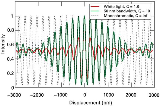
Note that for each wavelength (colour), a different pattern is formed. In practical white light interferometry, these colours can be visibly distinguished over a few wavelengths. White light interference is only possible in interferometers where the path difference can be made approximately zero.
The path length, ΔL, over which the interference remains visible, that is the visibility decreases by less than 50%, is called the coherence length and is given by
(4.8)
where λ0 is the wavelength of the light source and Q is the quality factor which determines over how many wavelengths interference is easily visible. Table 4.2 gives a few characteristics of known light sources.
Table 4.2
The Quality Factor and Coherence Length of Some Light Sources
| Light Source | Q | ΔL/m | λ0/nm | Colour |
| Bulb | 1.8 | 0.8×10⁻⁶ | 525 | White |
| Hg lamp | 1800 | 1×10⁻³ | 546 | Green |
| Cd lamp | 3.1×10⁵ | 0.2 | 644 | Red |
| 86Kr lamp | 1.4×10⁶ | 0.8 | 565 | Orange-red |
| He–Ne laser (multiple mode) | 8×10⁴ | 0.05 | 633 | Red |
| He–Ne laser (single mode) | 108 | 60 | 633 | Red |

In the early twentieth century, the cadmium spectral lamp was used for interference over macroscopic distances. Michelson’s determination of the cadmium lamp wavelength related to the metre standard was a breakthrough to a metre definition based on physical constants. The orange-red line of the 86Kr spectral lamp was used as the metre definition from 1963 until 1983. This definition was possible as, with some effort, interference over a metre length difference was possible and a length up to 1 m could be measured using interferometry.
4.4 Interferometer designs
For precision measurements, many interferometer types are used. It is important that for almost all types of interferometer the principles outlined in Section 4.3 are valid.
4.4.1 The Michelson and Twyman–Green interferometer
Where Michelson was a major pioneer in interferometry and carried out experiments that achieved major breakthroughs in physics, one often refers to a Michelson interferometer where in fact a Twyman–Green interferometer is intended. The original Michelson interferometer does not operate with collimated light, but with a point source, S, as shown in Figure 4.7.

A beam splitter, A, with a 50% coating splits the input beam. The interference fringes are detected from B. The compensator, C, is a glass plate with the same thickness as A which makes the optical path length through glass equal for both beams. This ensures that chromatic effects in the glass plate, A, are compensated and white light interferometry is possible.
Optically, the system as viewed from B consists of two sources, M1 and M2, behind each other. If the two image planes, M1 and M2, are parallel, this is equivalent to sources in line behind each other and one detects circular fringes. If M1 and M2 intersect, the crossover is the position of zero path difference and, as this region is a straight line of intersection, white light fringes will appear on the straight line of the intersection. The fringes appear to be localised at the front mirror, M1, that is the detector must be focused on this surface in order to obtain the sharpest fringes. With increasing displacement, the fringes become spherical because of the divergent light source.
4.4.1.1 The Twyman–Green modification
In the Twyman–Green modification to the Michelson interferometer, the source is replaced by a point source, S, at the focus of a well-corrected concave lens (Figure 4.8). The lens B collects the emerging light and the detector observes the interference pattern at the focal plane, D.

Consider the case where the mirror and its image are parallel. Now the collimated point source leads to a field of uniform intensity. Variations of this interferometer are the Köster gauge block interferometer [9], displacement measuring interferometers (see Section 5.2) and the Linnik- and Mirau-type interference microscopes (see Section 6.7.3.2).
An important characteristic of the Twyman–Green interferometer is that the paths in both beams can be made equal so that white light interference occurs. A disadvantage is that both beams have a macroscopic path length and can be sensitive to turbulence and vibration. The reflectivity of both mirrors can be up to 100%. If the reflectivity of the mirrors is different, the visibility decreases, as is illustrated in Figure 4.4. In the interferogram, the difference between the two mirrors is observed. For example, if both mirrors are slightly convex, and one mirror is slightly tilted, the interferogram will consist of straight lines (the same as with perfectly flat mirrors).
4.4.2 The Fizeau interferometer
In Fizeau interferometry, the reference surface and the surface to be measured are brought close together. Compared with Figure 4.3, mirror M1 is transparent and partially reflecting, and the partial reflecting side is positioned close and almost parallel to mirror M2. This gives a configuration as shown in Figure 4.9.

For a wedge angle, α, and perfectly flat mirrors, the intensity of the interference pattern between the mirrors is given by
(4.9)
where x is the position of the interference pattern from the left edge of the mirrors. In two dimensions, with circular mirrors, this gives a characteristic interference pattern consisting of straight lines (Figure 4.10).
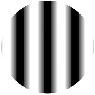
The Fizeau interferometer gives a direct way of observing geometrical features in an interferogram. If the distance ΔL is increased, the fringes will move from left to right (or right to left). If the tilt angle is changed, the distance between the fringes changes. If either of the mirrors is not flat, this is observed as distortions in the straightness of the fringes.
If the interference term in Eq. (4.9) can be changed in some controlled manner, the phase φ=2kΔL can be determined by making intensity measurements in one location (x, y). The phase can be changed by a small displacement, ΔL, or by a wavelength change. If ΔL is changed in four steps of λ/8 each, and the intensities are labelled as IA, IB, IC and ID, then it can be shown that
(4.10)
This is an example of deriving the phase, and ΔL, by phase stepping. This can only give an estimate of ΔL within an unknown integer number, N, of half wavelengths.
Considered over the surface, the distance between the surfaces S1 and S2 can be expressed as
(4.11)
If the upper surface deviations of both S1 and S2 are to be considered positive in the glass–air interface direction then, apart from a constant term and a constant tilt, the deviations can be expressed as
(4.12)
In S1, the coordinates can be (x, −y) or (−x, y), depending on the definition and the (flipping) orientation of the (optical) surface. However, in a Michelson interferometer for S1 the equivalent of S2 holds.
If S1 is perfectly flat, or has a known flatness deviation, the form of the other surface can be derived, either by visually observing the interference pattern or by analysing the phase using Eq. (4.11). This method of surface interferometry is a research field of its own and is covered in several textbooks (see Refs. [10,11]). Because the lateral resolution is usually limited, this is form rather than surface texture measurement. Uncertainties can be in the nanometre region in the direction perpendicular to the surface. Limitations are in the roughness and the maximum angle that can be measured. For engineered surfaces, this method is applicable for polished, and precision turned, lapped and ground surfaces. For such surfaces, Fizeau interferometry is a very powerful tool to obtain very rapidly the complete geometry of the surface.
Some characteristics of Fizeau interferometers should be mentioned, also in comparison to Michelson set-ups:
• White light interference is not possible; one always needs a light source with a coherence length of a few millimetres or more.
• The reference mirror must be partially transmitting, and the back side of this reference mirror should not interfere with its front side. This can be achieved by, for example an anti-reflection coating or by a wedge.
• If mirror S2 has a reflectivity of around 100%, it is difficult to achieve good visibility, as the reference mirror must be transmitting.
• The ambiguity of N can be a problem if it varies over the surface in a complicated way (i.e. the fringe pattern is complex and/or noisy). The determination of the proper variation in N over the surface can be complicated – this process is called phase unwrapping.
• As mirror S1 is held upside down, the interferometer measures the sum of the surface deviations of both surfaces. This enables an absolute flatness calibration when a third flat is used. However, because of the coordinate flipping, the measurement in all three combinations must be combined with additional rotations of one of the flats [12]. In a Michelson set-up, an absolute calibration is not possible.
• Instead of flats, spheres can be measured and, with some modifications, even parabolas can be measured. This is outside the scope of this book (but see Ref. [13]).
4.4.3 The Jamin and Mach–Zehnder interferometers
The Jamin interferometer is depicted in Figure 4.11. The beams are split in A and recombine at D. A first important application of the Jamin interferometer was the measurement of the refractive index of gases (T1 and T2 represent gas cells in Figure 4.11). The Jamin arrangement can also be used to make an image interfere with itself, but slightly displaced, for example by tilting one mirror relative to the other. This is called shearing interferometry.

A modification of the Jamin arrangement is known as the Mach–Zehnder interferometer and is depicted in Figure 4.12. As in the Michelson interferometer, white light interference is possible and there is no limitation to the reflectance at, for example, points C and F.

The Mach–Zehnder interferometer can be used for refractometry, that is for measurement of the refractive index of a medium in either arm. It can also be modified in order to enable displacement measurement.
4.4.4 The Fabry–Pérot interferometer
If in the Fizeau interferometer in Figure 4.9 both mirrors are placed almost parallel and the reflectance of both mirrors is increased, a particular type of interferometer is obtained, called the Fabry–Pérot interferometer (Figure 4.13).

Light enters from the left, and B and B′ are the reflecting faces between which the interference occurs. P and P′ are spacers to put flats B and B′ as parallel as possible. Between B and B′ multiple reflections occur. Equation (4.4) no longer holds if the reflectance, R, of both plates becomes significantly large, for example R>0.1. Summation of all reflected and transmitted components leads to an infinite series, which can be expressed as
(4.13)
where F is defined as
(4.14)
The reflectance of the whole system is given by R=1−T, where T is given by Eq. (4.13) and where it is assumed that no absorption takes place. The transmittance as a function of the distance, L, between the plates, for a wavelength λ=600 nm, is shown in Figure 4.14.

Figure 4.14 shows (co)sine-like behaviour similar to that described in Eq. (4.4) for low reflectances, but for high reflectance of the mirrors there are sharp transmittance peaks. This has the disadvantage that in between the peaks the position is difficult to estimate, but it has the advantage that once a peak reflectance is achieved, one is very sure that a displacement of exactly an integer number of half wavelengths has taken place.
The reciprocal of the full width of a fringe at half of the maximum intensity expressed as a fraction of the distance between two maxima is given by
(4.15)
The term NR is called the finesse of the interferometer. For example, for R=0.9, NR=30. This means that 1/30th of a half wavelength can readily be resolved by this interferometer; compare this to half of a half wavelength using the same criterion for the cosine function in Eq. (4.4).
At a fixed distance, L, the possible frequencies that fit in the cavity can be calculated as follows
(4.16)
Here m=0, 1, 2, … and n is the air refractive index, which is approximately 1. The frequency difference between two successive possible frequencies is called the free spectral range. For example, for a cavity length L=100 mm, Δf=1.5 GHz. Clearly, in a Fabry–Pérot interferometer, white light interferometry is not possible. The interferometer can also be made with spherical mirrors. In this case, the equation for the finesse changes somewhat. This and other details of the Fabry–Pérot interferometer are extensively treated in Ref. [14].
Fabry–Pérot interferometers have many applications in spectroscopy. However, in engineering nanometrology, they are used as the cavity in lasers and they can be used to generate very small, very well-defined displacements, either as part of a laser (the so-called measuring laser) or as an external cavity. This is treated in more detail in Section 5.10.1.
4.5 Measurement of gauge blocks by interferometry
4.5.1 Gauge blocks and interferometry
As discussed in Section 4.2, the length of a gauge block wrung to a platen can be measured using interferometry. The ISO definition of a gauge block length has a twofold purpose: (1) to ensure that the length can be measured by interferometry and (2) to ensure that there is no additional length due to wringing. An issue that is not obvious from the definition is whether the two-sided length of a gauge block after calibration by interferometry coincides with the mechanical length, for example as measured by mechanical probes coming from two sides. Up to now, no discrepancies have been found that exceed the measurement uncertainty, which is in the 10–20 nm range.
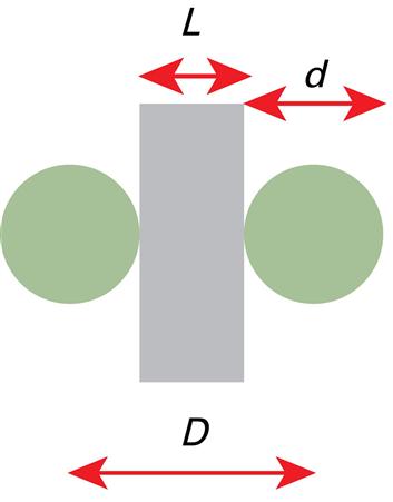
Figure 4.15 shows a possible definition for a mechanical gauge block length. A gauge block with length L is probed from both sides with a perfectly round probe of diameter d, being typically a few millimetres in diameter. The mechanical gauge block length, L, is the probe displacement, D, in the limit of zero force, minus the probe diameter, or L=D−d.
4.5.2 Gauge block interferometry
In order to measure gauge blocks in an interferometer, a first requirement for the light source is to have a coherence length that exceeds the gauge block length. Gauge block interferometers can be designed as a Twyman–Green or a Fizeau configuration, where the former is more common. For the majority of the issues discussed in this section, either configuration can be considered.
Figure 4.16 is a schema of a gauge block interferometer containing a gauge block. The observer sees the fringe pattern that comes from the platen as shown in Figure 4.10. If the platen has a small tilt, this will be a set of straight, parallel interference fringes. However, at the location of the gauge block, a parallel plate can also be observed, but the fringe pattern may be displaced (Figure 4.17).


If the fringes are not distorted, then an integer number of half wavelengths will fit in the length of the gauge block. In general this will not be the case, and the shift of fringes gives the fractional length of the gauge block. The length of the gauge block is given by
(4.17)
 (4.17)
where N is the number of half wavelengths between the gauge block top and the position on the platen for wavelength λ, n is the air refractive index and f is the fraction f=a/b in Figure 4.17. ϕblock (top) is the phase on top of the gauge block, ϕref (top area) is the phase at the reference plate at the location of the top area, ϕplaten (base) is the phase on the platen next to the gauge block and ϕref (base area) is the phase at the reference plate at the location next to the image of the gauge block. For a flat reference surface, the phase for the areas corresponding to the base and top of the gauge block is the same (ϕref (top area)=ϕref (base area)) and Eq. (4.17) simplifies accordingly. Equation (4.17) is the basic equation that links an electromagnetic wavelength, λ, to a physical, mechanical length, L.
Some practical issues that are met when applying Eq. (4.17) are treated in the next sections.
4.5.3 Operation of a gauge block interferometer
4.5.3.1 Fringe fraction measurement – phase stepping
As indicated in Figure 4.17, the fringe fraction can be estimated visually. For this purpose, as a visual aid, some fiducial dots or lines can be applied to the reference mirror. Experienced observers can obtain an accuracy of 5%, corresponding to approximately 15 nm.
However, more objective and accurate methods for determining the fringe fraction are possible by phase shifting; this means that the optical distance of either the reference mirror or the platen–gauge block combination is changed in a controlled way [15]. Established methods for phase shifting include:
• displacing the reference mirror or the gauge block with platen using piezoelectric displacement actuators;
• positioning an optical parallel in the beam. Giving the optical parallel a small rotation generates a small controllable phase shift.
Having the possibility of shifting the phase, the fraction can be derived in a semi-manual way. For example, the fringes on the platen can be adjusted to a reference line then on the gauge block, and then the next fringe on the platen can be adjusted to this reference line. Reading the actuator signal, or a rotary position of the optical parallel at these three settings, gives the possibility of deriving a fringe fraction, f.
Recording complete images and applying Eq. (4.9) is probably the most objective and accurate method to determine f. This is similar to Fizeau interferometry, although in this case it is usually done with multiple spectral or laser lines in a Michelson configuration.
4.5.3.2 Multiple wavelength interferometry analysis
If just a single fraction of a single wavelength is known, the gauge block length must be known beforehand within an uncertainty of 0.15 μm in order to define N in Eq. (4.17) within one integer unit. For gauge blocks to be calibrated this level of prior knowledge is usually not the case – see Table 4.1 – and it is common practice to solve this problem by using multiple wavelengths. In the original gauge block interferometers, this was usually possible as spectral lamps were used that emitted several lines with an appropriate coherence length. In modern interferometers, laser sources are normally used, and the demand for multiple wavelength operation is met with multiple laser sources.
For multiple wavelengths, λi (i=1, 2, …), Eq. (4.17) can be rewritten as
(4.18)
However, because of a limited uncertainty in the fringe fraction determinations, there is not a single length that can meet the requirements of Eq. (4.18) for all wavelengths and fractions. There are several strategies for finding an optimal solution for the length; for example, for the longest wavelength, a set of possible solutions around the nominal length can be taken and for each of these lengths the closest solution for the possible lengths for the measurements at the other wavelengths can be calculated. The average of the length with the least dispersion is then taken as the final value. This method is known as the method of exact fractions and has similarities with reading a vernier on a ruler.
More generally, Eq. (4.18) can be written as a least-squares problem. The error function is given by
(4.19)
where K is the number of wavelengths used and Le is the estimated length. For ideal measurements, χ2=0 for Le=L. For real measurements, the best estimate for L is the value for Le where χ2 is minimal. For any length, Le, first the value of Ni that gives a solution closest to L has to be calculated for each wavelength before calculating χ2. As Eq. (4.19) has many local minima (every 0.3 μm), it must be solved by a broad search around the nominal value, for example as was implicitly done in the procedure described above. To distinguish between two adjacent solutions, the fringe fractions must be determined accurately enough. This demand is higher if the wavelengths are closer together. For example, for wavelength λ1=633 nm (red) and λ2=543 nm (green), the fractions must be determined within 15% in order to ensure that a solution that is 0.3 μm in error is not found.
Multiple wavelengths still give periodic solutions where χ2 is minimal, but instead of 0.3 μm, these are further apart; in the example of the two wavelengths just given, this period becomes 2.5 μm. If two wavelengths are closer together, the demand on the accuracy of the fringe fraction determination is increased accordingly, and the period between solutions increases.
Using more than two wavelengths further increases the period of the solutions; the wavelength range determines the demand on the accuracy of the fraction determination. A common strategy for obtaining an approximate value for Le, with an uncertainty at least within the larger periodicity, is to carry out a mechanical comparison with a calibrated gauge block.
4.5.3.3 Vacuum wavelength
The uncertainty in the length of a gauge block measured by interferometry directly depends on the accuracy of the determination of the vacuum wavelength. In the case of spectral lamps, these are more or less natural constants, and the lines of krypton and cadmium are (still) even defined as primary standards. Stabilised lasers must be calibrated using a beat measurement against a primary standard, as described in Section 2.9.5. When using multiple wavelengths, especially for larger lengths up to 1 m, a small deviation of the vacuum wavelength can cause large errors because a solution is found one or more fringe numbers in error. For example, for a 1 m gauge block, an error of 4×10⁻⁸ in wavelength will result in the wrong calculated value for N such that the error is 3×10⁻⁷ (one fringe in a metre). This limits the maximum length that can be determined depending on the accuracy of the wavelengths.
When using a frequency comb [16,17] (see also Section 2.9.6), the uncertainty in the vacuum wavelength will be negligible compared to other factors. Formally, it sounds very good that the calibration is directly traceable to a primary standard, but for the uncertainty, the other factors mentioned are more important.
4.5.3.4 Thermal effects
The reference temperature for gauge block measurements is defined in the specification standard ISO 1 [18] to be 20°C, exactly. The reason that it is necessary to specify a temperature is because all gauge blocks will change size when their temperature changes due to thermal expansion. The amount by which the material changes length per degree temperature change is the coefficient of thermal expansion, α. For a typical steel gauge block, the coefficient of thermal expansion is about 11.5×10⁻⁶ K−1 and for a tungsten carbide gauge block it is nearer 4.23×10⁻⁶ K−1.
In order to correct for the change in length due to thermal expansion, it is necessary to measure the temperature of the gauge block at the same time as the length is being measured. The correction factor can be derived from
(4.20)
where L(T) is the length at temperature, T (in degrees Celsius), and L(20) is the length at 20°C.
Equation (4.20) indicates that an accurate temperature measurement is more critical when α is large and that knowledge of α is more critical if the temperature deviates from 20°C. For example, for a one part per million per degree Celsius error, Δα, in the expansion coefficient, the error is 100 nm for a 100 mm gauge block at 21°C. For α=10×10−6 K−1, a 0.1°C uncertainty in the temperature gives 100 nm uncertainty in a 100 mm gauge block.
4.5.3.5 Refractive index measurement
The actual wavelength depends on the frequency and the refractive index of the air in the path adjacent to the gauge block. In very accurate interferometers, for long gauge blocks, the refractive index is measured directly by a refractometer that may effectively be described as a transparent gauge block containing a vacuum.
The refractive index of air is directly related to the air density, which itself is influenced by:
The last of these influences, other gases, has a negligible effect and can usually be ignored. So we need to measure the air temperature, air pressure and humidity. We then use well-known equations to calculate the air refractive index from these measured parameters.
These equations go by several names, depending on the exact equations used, and are known by the names of the scientists who derived them. Examples include Edlén [19], Birch and Downs (also known as the modified Edlén equation) [20,21], Ciddor [22] and Bönsch [23]. NIST has published all the equations and considerations on their website, including an online calculator: see emtoolbox.nist.gov/Wavelength/Abstract.asp. It may be useful to note the sensitivity of the refractive index to these various parameters, as given in Table 4.3.
Table 4.3
Effect of Parameters on Refractive Index
| Effect | Sensitivity | Variation Needed for Change of 10 nm in 100 mm |
| Air pressure | 2.7×10⁻⁷ L/mbar | 0.37 mbar |
| Air temperature | 9.3×10⁻⁷ L/°C | 0.11°C |
| Air humidity | 1.0×10⁻⁸ L/% RH | 10% RH |
| Wavelength | 2.0×10⁻⁸ L/nm | – |
From Table 4.3, it can be seen that if one wishes to reduce the contribution of these potential error sources to below 1×10⁻⁷ L (i.e. 10 m in 100 mm length), then one needs to make air pressure measurement with an uncertainty below 0.4 mbar, air temperature measurement to better than 0.1°C and air humidity measurement to better than 10% RH (relative humidity). Such measurements are not trivial but well achievable with commercial instruments. The wavelength also needs to be known accurately enough – within small fractions of a nanometre (it is mentioned here for completeness, as the refractive index is also wavelength dependent).
4.5.3.6 Aperture correction
A subtle optical effect that is less obvious than the previous uncertainty influences is the so-called aperture correction. The figures in Section 4.4 show the light sources as point sources, but in reality a light source has a finite aperture. This means that light does not only strike the gauge block and reference plane exactly perpendicular, but also at a small angle. This makes the gauge block appear shorter than it really is. The correction for this effect for a circular aperture is given by
(4.21)
where D is the aperture and f is the focal length of the collimating lens. Taking some typical numbers, D=0.5 mm, f=200 mm, L=100 mm, we find ΔL=0.04 μm. This correction is much larger in the case of an interference microscope, where it may amount to up to 10% of the measured height (see Section 6.7.1).
In some interferometer designs, there is a small angle between the impinging light and the observed light that gives rise to a similar correction known as the obliquity correction.
4.5.3.7 Surface and phase change effects
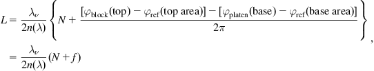
As indicated in the gauge block definition, the gauge block has to be wrung on to a platen having the same material and surface roughness properties as the gauge block. In practice, this can be approached but never guaranteed. Sometimes glass or quartz is preferred as a platen because the wringing condition can be checked through the platen. Because of the complex refractive index of metals, light effectively penetrates into the material before being reflected, so a metal gauge block on a glass platen will be measured as too short. Additional to this is the gauge block roughness effect. Typical total correction values are 0.045 μm for a steel gauge block on a glass platen and 0.01 μm for a tungsten carbide gauge block on a glass platen.
A very practical way of determining the surface effects is wringing a stack of two (or more) gauges together on a platen and comparing the length of the stack to the sum of the individually measured gauge blocks.
This is illustrated for two gauge blocks in Figure 4.18, where g and p are the apparent displacements of the optical surface from the mechanical surface, f is the wringing film thickness and Li are the defined (mechanical) lengths of individual gauges. It can be shown that the measured length of the combined stack minus the individual measured length is the correction per gauge. This method can be extended to multiple gauge blocks to reduce the uncertainties. Here it is assumed that the gauge blocks are from the same material and have nominally the same surface texture.
Other methods for measuring corrections for surface effects of the gauge block and platen have been proposed and are used in some NMIs (see, for example Ref. [24]). Such methods can offer a slightly reduced uncertainty for the phase correction but are often difficult to set up and can give results that may be difficult to interpret.
4.5.4 Sources of error in gauge block interferometry
In this section, some more detailed considerations are given on the errors generated by the different factors mentioned in Section 4.5.3 (see Ref. [25] for a more thorough treatment).
4.5.4.1 Fringe fraction determination uncertainty
The accuracy of the fringe fraction determination is governed by the repeatability of the measurement process, the quality of the gauge block and the flatness and parallelism of the end faces. With visual fringe fraction determination, an uncertainty of 5%, corresponding to approximately 15 nm, is considered as a limit. With photoelectric determination, this limit can be reduced to a few nanometres; however, the reproducibility of the wringing process is of the same order of magnitude.
4.5.4.2 Multi-wavelength interferometry uncertainty
As previously mentioned, the determination of the correct interference order is the main issue when using multiple wavelength interferometry. For this purpose, it is absolutely necessary that the fringe fractions are determined within 10–15%. Once the fringe fractions are less sure, the measurement becomes meaningless. Also a correct predetermination of the gauge block length, for example by mechanical comparison, is essential if the gauge block is being calibrated for a first time.
4.5.4.3 Vacuum wavelength uncertainty
The uncertainty in the wavelength used is directly reflected in the calculated length, so long as the fringe order is uniquely defined. Stabilised lasers need periodic re-calibration, preferably against a primary standard. If one laser is calibrated, other lasers can be calibrated using gauge blocks – from a known length and measured fraction, the real wavelength of a light source can be measured. An unknown fringe order now leads to a possible number of wavelengths. By repeating the procedure for different gauge block lengths, a wavelength can be uniquely determined [26].
4.5.4.4 Temperature uncertainty
The temperature measurement is essential, and, if the temperature is different from 20°C, the expansion coefficient must also be known. Most temperature sensors can be calibrated to low uncertainties – calibration of a platinum-resistance thermometer to 0.01°C is not a significant problem for a good calibration laboratory. The problem with temperature measurement of a material is that the temperature of the material must be transferred to the sensor. This depends on thermal conductivity, thermal equilibrium with the environment, self-heat of the sensor and other factors. For this reason, long waiting times and multiple sensors attached to longer gauge blocks (L>100 mm) are common.
An approach that was already used in the first gauge block interferometers is to have a larger thermally conductive block near the gauge block. This block is measured with an accurate absolute sensor, and the difference of the gauge block with this reference block is determined by a thermocouple.
For the highest uncertainties, the uncertainty in the temperature scale becomes relevant; for example when ITS-90 was introduced in 1990 [27], the longest gauge blocks made a small but significant jump in their length.
4.5.4.5 Refractive index uncertainty
If the refractive index is established by indirect measurement of the air parameters, it is dependent on the determination of these parameters and in addition a small uncertainty of typically 2×10⁻⁸ in the Eq. (4.19) itself must be taken into account. The air temperature measurement may be most problematic because of possible self-heating of sensors that measure air temperature. Also, when the air temperature is different from the gauge block temperature, it is questionable exactly what is the air temperature near the gauge block that is measured.
4.5.4.6 Aperture correction uncertainty
As the aperture correction is usually small, an error in this correction does not necessarily have dramatic consequences. If possible, the aperture can be enlarged or reduced to check whether the estimate is reasonable. The same applies for the obliquity effect if there is a small angle between the beams.
4.5.4.7 Phase change uncertainty
Proper determination of the phase change correction is transferred to many measurements, so it is important to do multiple measurements with multiple gauge blocks in order to avoid making a systematic error when correcting large amounts of gauge blocks with the same value. For this determination, it is customary to take small gauge blocks that can be wrung well (e.g. 5 mm) so that length-dependent effects (refractive index, temperature) are minimal, and the fringe fraction determination and wringing repeatability are the determining factors.
4.5.4.8 Cosine error
Cosine error is mainly mentioned as an illustration of how closely the Abbe principle is followed by gauge block interferometry (see Section 5.2.8.3 for a description of the cosine error). The gauge block has to be slightly tilted in order to generate a number of fringes over the surface (with phase stepping this is not required). Even if 10 fringes are used over the gauge block length this gives a cosine error of 5×10⁻⁹ L, far within effects of common temperature uncertainties.
4.5.5 Alternative approaches
The need for wringing gauge blocks to a platen and let this stabilise is labour- and time consuming. For this reason, alternative interferometric methods have been developed. The basic idea is that both sides of a gauge block can be measured interferometrically, either in a single triangular interferometer or by two Twyman–Green interferometers from both sides simultaneously. Special care has to be taken for both the length determination and the phase correction. The phase correction that is necessary as the gauge block length is not measured according to its definition is often considered as the essential drawback; however, this phase correction needs to be determined anyhow so this should not be considered as so essential.
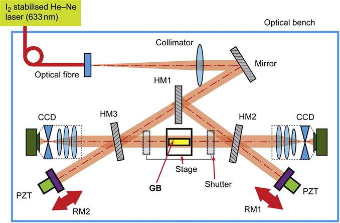
A fully operational double-sided gauge block interferometer was developed elsewhere [28]. The schema is given in Figure 4.19. The light is reflected from two reference mirrors (RM1, RM2) to create interference patterns from both ends of the gauge block (GB), as well as combinations of the total cavity length with the gauge block length, from which the absolute gauge block length can be derived. Abdelaty [29] has shown for a similar set-up that there are challenges, especially as the phase correction has to be applied twice and its uncertainty contributes accordingly, and additional mirrors and beam splitters of high quality are needed. Another approach was taken by Winarno et al. [30], who combine a double-sided interferometer in a triangle configuration with a displacement measurement that can be carried out remotely. In this case, the uncertainty of traditional gauge block interferometry has not yet been achieved.
The absence of wringing will mean shorter measurement times, less risk of scratches and wringing errors, and may make the interferometric gauge-stabilisation block calibration far more economic.
Using a frequency comb (see Section 2.9.6) opens up some interesting new possibilities [16,17], where a beam full of well-defined frequencies can be used both as a white light source that defines an absolute position in space, and as an accurate distance and/or displacement measurement that can be combined to an absolute gauge block length in single- and double-sided set-ups.