
Some Basics of Measurement
Richard Leach
This chapter introduced many of the basic concepts in the field of metrology. The international SI system is discussed along with the units of measurement. The units most used in engineering metrology, length, mass, force and angle, are then addressed in some detail, including their realisation. The important concept of traceability is then covered, including some examples, and the most important terms in metrology are introduced. Uncertainty in measurement is discussed, both the standard technique to estimate it and a Monte Carlo method. The theory and realisation of the laser are covered in some detail, including stabilisation schemes and the use of the laser to realise length.
Keywords
Système International d'Unités (SI); Units of Measurement; Length; Mass; Force; Angle; Traceability; Accuracy; Precision; Resolution; Error; Uncertainty; Monte Carlo; Laser
2.1 Introduction to measurement
Over the last couple of thousand years, significant advances in technology can be traced to improved measurements. Whether we are admiring the engineering feat represented by the Egyptian pyramids, or the fact that in the twentieth century humans walked on the moon, we should appreciate that this progress is due in no small part to the evolution of measurement. It is sobering to realise that tens to hundreds of thousands of people were involved in both operations and that these people were working in many different places producing various components that had to be brought together – a large part of the technology that enabled this was the measurement techniques and standards that were used [1] (see Ref. [2] for a historical account of measurement).
The Egyptians used a royal cubit as the standard of length measurement (it was the distance from Pharaoh’s elbow to his fingertips, plus the width of the palm – Figure 2.1), while the Apollo space programme ultimately relied on the definition of the metre in terms of the wavelength of krypton 86 radiation.

In Egypt, the standards were kept in temples, and the priests were beheaded if they were not re-calibrated on time. Nowadays, there are worldwide systems of accreditation agencies, and laboratories are threatened with losing their accreditation if the working standards are not re-calibrated on time. Primary standards are kept in national measurement institutes (NMIs) that have a great deal of status and national pride. The Egyptians appreciated that, provided that all four sides of a square are the same length and the two diagonals are equal, the interior angles will all be the same – 90°. They were able to compare the two diagonals and look for small differences between the two measurements to determine how square the base of the pyramid was.
Humans have walked on the moon because a few brave people were prepared to sit on top of a collection of three million manufactured parts all built and assembled by the lowest bidder, and finally filled with hundreds of tonnes of explosive hydrogen and oxygen propellant. A principal reason that it all operated as intended was that the individual components were manufactured to exacting tolerances that permitted final assembly and operation as intended.
The phrase ‘mass production’ these days brings visions of hundreds of cars rolling off a production line every day. From Henry Ford in the 1920s through to the modern car plants operated by companies such as BMW and Honda, the key to this approach is to have tiers of suppliers and subcontractors all sending the right parts to the next higher tier and finally to the assembly line. The whole manufacture and assembly process is enabled by the vital traceable measurements that take place along the route. This approach has now been taken up by the aerospace industry, and enormous aeroplanes are now assembled using structures and components transported to Toulouse from several countries.
Modern manufacturing often involves the miniaturisation of products and components. This ‘nanotechnology revolution’ has meant that not only have the parts shrunk to micrometres and nanometres, but tolerances can be shrunken too. The dimensional and mass measurements that are required to ensure that these tiny parts fit together, or ensure that larger precision parts are fit for purpose, are the subject of this book.
2.2 Units of measurement and the SI
The language of measurement that is universally used in science and engineering is the Système International d’Unités (SI) [3]. The SI embodies the modern metric system of measurement and was established in 1960 by the 11th Conférence Générale des Poids et Mesures (CGPM). The CGPM is the international body that ensures wide dissemination of the SI and modifies the SI as necessary to reflect the latest advances in science and technology. There are a number of international organisations, treaties and laboratories that form the scientific and legal infrastructure of measurement (see Ref. [4] for details). Most technologically advanced nations have NMIs that are responsible for ensuring that measurements comply with the SI and ensure traceability (see Section 2.7). Examples of NMIs include the National Physical Laboratory (NPL, UK), Physikalisch-Technische Bundesanhalt (PTB, Germany), National Metrology Institute Japan (NMIJ, Japan) and the National Institute of Standards and Technology (NIST, USA). The websites of the larger NMIs all have a wealth of information on measurement and related topics.
The SI is principally based on a system of base quantities, each associated with a unit and a realisation. A unit is defined as a particular physical quantity, defined and adopted by convention, with which other particular quantities of the same kind are compared to express their value. The realisation of a unit is the physical embodiment of that unit, which is usually performed at an NMI. The seven base quantities are given in Table 2.1. Engineering metrology is mainly concerned with length and mass, and these two base quantities will be given some attention here. Force and angle are also important quantities in engineering metrology and will be discussed in this chapter. The other base quantities, and their associated units and realisations, are presented in Appendix A.
Table 2.1
| Physical Quantity | Name of Unit | Abbreviation |
| Length | metre | m |
| Mass | kilogram | kg |
| Time | second | s |
| Electrical current | ampere | A |
| Amount of substance | mole | mol |
| Temperature | kelvin | K |
| Luminous intensity | candela | cd |
In addition to the seven base quantities, there are a number of derived quantities that are essentially combinations of the base units. Some examples include acceleration (unit: metres per second), density (unit: kilogram per cubic metre) and magnetic field strength (unit: ampere per metre). There are also a number of derived quantities that have units with special names. Some examples include frequency (unit: hertz or cycles per second), energy (unit: joule or kilogram per square metre per second) and electric charge (unit: coulomb or the product of ampere and second). Further examples of derived units are presented in Appendix B.
2.3 Length
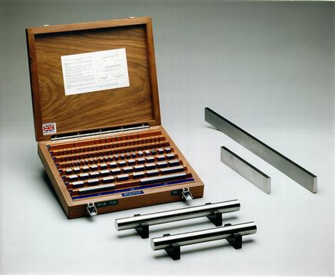
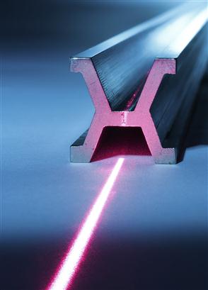
The definition and measurement of length has taken many forms throughout human history (see Refs. [2,5,6] for more thorough historical overviews). The metre was first defined in 1791, as one ten millionth of the polar quadrant of the earth passing through Paris. The team of surveyors that measured the part of the polar quadrant between Dunkirk and Barcelona took 6 years to complete the task. This definition of the metre was realised practically with a provisional metre bar of brass in 1795, with the metre defined as the length between the end faces of the bar. The brass bar was later replaced by a bar of platinum (a more stable material) in 1799. This illustrates the trade-offs between physical stability and reproducibility and the practical realisability of standards. Of course the earth’s quadrant is far more stable than a human’s arm length, but to realise this in a standard is much more tedious. Some years after the prototype metre was realised, some errors were found in the calculation of its length (from the survey results) and it was found that the platinum metre bar was about 1 mm short [2]. However, it was decided to keep the material artefact for practical reasons. Another struggle that has continued until today is the preference of material length; whether to use an end standard (see Section 4.2 and Figure 2.2) with two flat faces that define a distance or a line standard where two lines engraved in a material define a length. In 1889, the platinum metre was replaced by a platinum–iridium line standard, the so-called X-section (or Tresca) metre, which kept the same defined distance as well as possible (Figure 2.3).
The X-section metre was used until 1960 [7], when the metre was redefined as:
the metre is the length equal to 1 650 763.73 wavelengths in vacuum of the radiation corresponding to the transition between the levels 2p10 and 5d5 of the krypton 86 atom.
This redefinition was possible because of the developments in interferometry and the sharp spectral line of the krypton atom that enabled interferometry up to 1 m – allowing comparison of the wavelength of the krypton line with material standards such as gauge blocks (see Chapter 4). Around 1910, such a redefinition was proposed, but at that time the metre could not be reproduced with a lower uncertainty than with the material artefact.
In 1983, advances in the development of the laser, where many stabilisation methods resulted in lasers that were more stable than the krypton spectral line, led to the need for a new definition. In the meantime, it was found that the speed of light in a vacuum is constant within all experimental limits, independent of frequency, intensity, source movement and time. Also it became possible to link optical frequencies to the time standard, thereby allowing for simultaneous measurement of both the speed and the wavelength of light. This enabled a redefinition of the metre, which (as paraphrased by Petley [8]) became:
the length of the path travelled by light in a vacuum in a time interval of 1/c of a second, where c is the speed of light given by 299 792 458 m s−1.
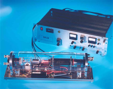
Together with this definition, a list of reference optical frequencies was given, with associated uncertainties [9], which became the accepted realisation of the metre, when suitable light sources were constructed and operated according to laid down specifications. These included spectral lamps, for example. The value for the krypton spectral line was unchanged but it received an attributed uncertainty. More convenient and precise, however, are stabilised laser systems. Such a current realisation of the metre can have an uncertainty in frequency of one part in 1011. Figure 2.4 shows an iodine-stabilised helium–neon laser held at NPL.
As discussed, the speed of light in a vacuum is generally regarded as a universal constant of nature, therefore, making it ideal as the basis for a length standard. The speed of an electromagnetic wave is given by
(2.1)
where ν is the frequency and λ is the wavelength of the radiation. Therefore, length can be disseminated by measuring frequency or wavelength, usually using either time of flight measurements or interferometry (see Chapter 4). For short distances (up to a few tens of metres) measurement is usually referred to the wavelength of the light, for example by counting interference fringes. For longer ranges (kilometres up to Earth–lunar distances, time of flight, i.e. velocity-based measurements are more practical). Note that length can be considered to be a base quantity that is realised in a manner that is based upon the principles of quantum mechanics. The emission of electromagnetic waves from an atom (as occurs in a laser – see Section 2.9) is a quantised phenomenon and not subject to change provided certain conditions are kept constant. This is a highly desirable property of a base unit definition and realisation [10].
Most of the measurements that are described in this book are length measurements. Displacement is a change in length, surface profile is made up of height and lateral displacement, and coordinate measuring machines (CMMs, see Chapter 9) measure the three-dimensional geometry of an object. However, philosophically, the modern definition of length has become dependent on the definition of time, but in practice this simply means that the two units are related by a fundamental constant – the speed of light – fixing one of the units ties down the other, provided that the value of the fundamental constant is known (in the relevant units). Relating length to a standard of time was proposed earlier; in the seventeenth century, Christiaan Huygens proposed to define the metre as the length of a bar with a time of oscillation of one second [2]. However, this failed because of the variation of local acceleration due to gravity with geographic location.
Recent advances in lasers and non-linear optics underpinned the Nobel Prize winning work which led to the use of femtosecond lasers and optical frequency combs as a tool which can be used to compare and link frequencies from across the electromagnetic spectrum. With a so-called femtosecond comb, the frequency standard from an atomic clock can be directly coupled to optical frequencies such as those emitted by stabilised lasers, removing the requirement for the laborious frequency chain comparisons from the 1970s, which Blaney [11,12] used to provide values for input into Eq. (2.1). Femtosecond combs are now accepted as ways of realising the metre, and they are used routinely for calibration of other laser systems.
Chiefly driven by the lack of stability of the realisation of the SI kilogram (see Section 2.4 and Chapter 10), a revision of all the SI base unit definitions is planned to take place at the same time as the redefinition of the kilogram, and then the scale of the SI will be based on seven fixed constants: the ground state hyperfine splitting of the caesium atom (Δν(133Cs)hfs), the speed of light in a vacuum (c), the Planck constant (h), the elementary charge (e), the Boltzmann constant (k), the Avogadro constant (NA) and the luminious efficacy (Kcd) of radiation of frequency 530×1012 Hz.
Fortunately, the metre is already defined in terms of the speed of light, so although the exact wording of the definition may change, the fundamental constant on which it is based, and the physical length, will remain the same.
2.4 Mass
In 1790, Louis XVI of France commissioned scientists to recommend a consistent system for weights and measures (see Refs. [13,14] for more thorough historical overviews of mass metrology). In 1791, a new system of units was recommended to the French Academy of Sciences, including a unit that was the mass of a declared volume of distilled water in vacuo at the freezing point (which was soon succeeded by a cubic decimetre of water at 4°C – at which temperature water is most dense). This unit was based on natural constants but was not reproducible enough to keep up with technological advances. Over the next hundred years, this definition of a mass unit was refined and a number of weights were manufactured to have a mass approximately equal to the mass unit. In 1879, Johnson Matthey and Co. of London successfully cast an ingot of an alloy of platinum and iridium, a highly stable material. The water definition was abandoned, and the platinum–iridium weight became the standard kilogram (known as the International Prototype of the Kilogram). In 1889, 40 copies of the kilogram were commissioned and distributed to the major NMIs to be their primary standard. The United Kingdom received Kilogram 18, which is now held at NPL (Figure 2.5). The International Prototype of the Kilogram is made of an alloy of 90% platinum and 10% iridium and is held at the Bureau International des Poids et Mesures (BIPM) in Paris, France. A thorough treatise on mass metrology is given in Chapter 10.
Whereas the definition of length is given in terms of fundamental physical constants, and its realisation is in terms of quantum mechanical effects, mass does not have these desirable properties. All mass measurements are traced back to a macroscopic physical object. The main problem with a physical object as a base unit realisation is that its mass could change due to loss of material or contamination from the surrounding environment. The International Prototype of the Kilogram’s mass could be slightly greater or less today than it was when it was made in 1884, but there is no way of proving this [15]. It is also possible that a physical object could be lost or damaged. For these reasons, there is considerable effort worldwide to redefine mass in terms of fundamental physical constants [16,17]. The front-runners at the time of writing are the Watt balance, based on electrical measurements that can be realised in terms of Planck’s constant and the charge on an electron [16,18], and the Avogadro method, based on counting the number of atoms in a sphere of pure silicon and determining the Avogadro constant [19]; more methods are described in Section 10.1.6. As with the metre, it is easy to define a standard (e.g. mass as a number of atoms) but as long as it cannot be reproduced better than the current method, a redefinition, even using well-defined physical constants, does not make sense.
On the micro- and nanotechnology (MNT) scale, masses can become very small and difficult to handle. This makes them difficult to manipulate, clean and ultimately calibrate. Also, atom level forces can become significant. These difficulties are discussed in the following section, which considers masses as force production mechanisms (weights).
2.5 Force
The SI unit of force, a derived unit, is the newton – one newton is defined as the force required to accelerate a mass of one kilogram at a rate of one metre per second – per second. The accurate measurement of force is vital in many MNT areas, for example the force exerted by an atomic force microscope on a surface (see Section 7.3.5), the thrust exerted by an ion thrust space propulsion system [20] or the surface forces that can hamper the operation of devices based on microelectromechanical systems (MEMS) [21].
Conventionally, force is measured using strain gauges, resonant structures and load cells (www.npl.co.uk/upload/pdf/forceguide.pdf). The calibration of such devices is carried out by comparison to a weight. If the local acceleration due to gravity is known, the downward force generated by a weight of known mass can be calculated (the volume of the mass and the density of the air also need to be known for an accurate measurement). This is the principle behind deadweight force standard machines – the mass values of their internal weights are adjusted so that, at a specific location, they generate particular forces. At NPL, gravitational acceleration is 9.81182 m·s−2, so a steel weight with a mass of 101.9332 kg will generate a downward force of approximately 1 kN when suspended in air. Forces in the meganewton range are generated using large deadweight machines, and forces above this tend to be generated hydraulically – oil at a known pressure pushes on a piston of known size to generate a known force [22].
When measuring forces on the MNT scale, different measurement principles are applied compared to the measurement of macroscale forces. As mass values decrease, their relative uncertainty of measurement increases. For example, at NPL, a 1 kg mass can be measured with a standard uncertainty of approximately 1 μg or 1 part in 109. However, a 1 mg mass can only be measured with a standard uncertainty of approximately 0.1 µg or 1 part in 104, a large difference in relative uncertainty. This undesired scaling effect of mass measurements is due to the limitations of the instrumentation used and the small physical size of the masses, but is mainly because of the subdivision method used to achieve traceability back to the SI unit (the kilogram). Such small masses are difficult to handle and attract contamination easily (typically dust particles have masses ranging from nanograms to tens of micrograms). The limitation also arises because the dominant forces in the measurement are those other than gravitational forces. Figure 10.2 shows the effects of the sort of forces that are dominant in interactions on the MNT scale. Therefore, when measuring force from around 1 μN or lower, alternative methods to mass comparison are used, for example the deflection of a spring with a known spring constant. Chapter 10 details methods that are commonly used for measuring the forces encountered in MNT devices along with a description of endeavours around the world to ensure the traceability of such measurements.
2.6 Angle
The SI regards angle as a dimensionless quantity (also called a quantity of dimension one). It is one of a few cases where a name is given to the unit one, in order to facilitate the identification of the quantity involved. The names given for the quantity angle are radian (plane angle) and steradian (solid angle). The radian is defined with respect to a circle and is the angle subtended by an arc of a circle equal to the radius (approximately 57.2958°).
For practical angle measurement, however, the sexagesimal (degrees, minutes, seconds) system of units, which dates back to the Babylonian civilisation, is used almost exclusively [23]. The centesimal system introduced by Lagrange towards the end of the eighteenth century is rarely used.
Other units referred to in this section require either a material artefact (e.g. mass) or a natural standard (e.g. length). No ultimate standard is required for angle measurement since any angle can be established by appropriate subdivision of the circle. A circle can only have 360°.
In practice, basic standards for angle measurement depend either on the accurate division of a circle or on the generation of an angle from two known lengths. Instruments that rely on the principle of subdivision include precision index tables, rotary tables, polygons and angular gratings [23]. Instruments that rely on the ratio of two lengths include angular interferometers (see Section 5.2.9), sine bars, sine tables and small angle generators. Small changes in angle are detected by an autocollimator [24] used in conjunction with a flat mirror mounted on the item under test, for example a machine tool (Figure 2.6). Modern autocollimators give a direct digital readout of angular position. The combination of a precision polygon and two autocollimators enables the transfer of high accuracy in small angle measurement to the same accuracy in large angles, using the closing principle that all angles add up to 360°.

Sometimes angle measurement needs to be gravity referenced and in this case use is made of levels. Levels can be based either on a liquid-filled vial or on a pendulum and ancillary sensing system.
2.7 Traceability
The concept of traceability is one of the most fundamental in metrology and is the basis upon which all measurements can be claimed to be accurate. Traceability is defined as follows:
Traceability is the property of the result of a measurement whereby it can be related to stated references, usually national or international standards, through a documented unbroken chain of comparisons all having stated uncertainties [25].
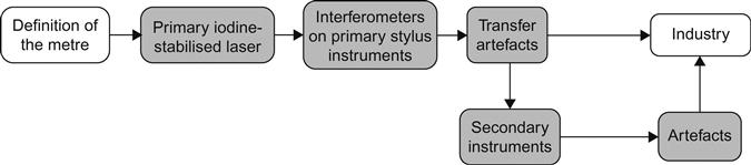
To take an example, consider the measurement of surface profile using a stylus instrument (see Section 6.6.1). A basic stylus instrument measures the topography of a surface by measuring the displacement of a stylus as it traverses the surface. So, it is important to ensure that the displacement measurement is ‘correct’. To ensure this, the displacement-measuring system must be checked or calibrated against a more accurate displacement-measuring system. This calibration can be carried out by measuring a calibrated step height material measure (known as a transfer artefact). Let us assume that the more accurate instrument measures the displacement of the step using an optical interferometer with a laser source. This laser source is calibrated against the iodine-stabilised laser that realises the definition of the metre [8,9], and an unbroken chain of comparisons has been assured. Moving down the chain from the definition of the metre to the stylus instrument that is being calibrated, the accuracy of the measurements usually decreases (Figure 2.7).
It is important to note the last part of the definition of traceability that states all having stated uncertainties. This is an essential part of traceability as it is impossible to usefully compare, and hence calibrate, instruments without a statement of uncertainty. This fact should become obvious once the concept of uncertainty has been explained in Section 2.8. Uncertainty and traceability are inseparable. Note that in practice the calibration of a stylus instrument is more complex than making a simple displacement measurement (see Section 6.10).
Traceability ensures that measurements are consistent and accurate. Any quality system in manufacturing will require that all measurements are traceable and that there is documented evidence of this traceability (e.g. ISO 17025 [26]). If component parts of a product are to be manufactured by different companies (or different parts of an organisation), it is essential that measurements are traceable so that the components can be assembled and integrated into a product.
In the case of dimensional nanometrology, there are many examples when it is not always possible to ensure traceability because there is a break in the chain, often at the top of the chain. There may not be national or international specification standards available and the necessary measurement infrastructure may not have been developed [27]. This is the case for many complex three-dimensional MNT measurements. Also, sometimes an instrument may simply be too complex to ensure traceability of all measurements. An example of this is the CMM (see Chapter 9). Whilst the scales on a CMM (macro- or micro-scale) can be calibrated traceably, the overall instrument performance, or volumetric accuracy, is difficult and time consuming to determine and will be task specific. In these cases, it is important to verify the performance of the instrument against its specification by measuring artefacts that have been traceably calibrated in an independent way. Where there are no guidelines, or where there is a new measurement instrument or technique to be used, the metrologist must apply good practice and should consult other experts in the field.
Traceability does not only apply to displacement (or length) measurements – all measurements should be traceable to their respective SI unit. In some cases, for example in a research environment or where a machining process is stable and does not rely on any other process, it may only be necessary to have a reproducible measurement. In this case, the results should not be used where others may rely upon them and should certainly not be published.
2.8 Accuracy, precision, resolution, error and uncertainty
There are many terms used in metrology, and it is important to be consistent in their use. The International vocabulary of metrology – Basic and general concepts and associated terms (popularly known as the VIM) [25] lays out formal definitions of the main terms used in metrology. Central to many metrology terms and definitions is the concept of the true value (sometimes referred to as the true quantity value or the true value of a quantity). The true value is defined in VIM as the quantity value consistent with the definition of a quantity and is the hypothetical result that would be returned by an ideal measuring instrument if there were no errors in the measurement. In practice, the perfect scenario can never be achieved; there will always be some degree of error in the measurement and it may not always be possible to have a stable, single-valued measurand. Even if an ideal instrument and measurement set-up were available, all measurements are ultimately subject to Heisenberg’s Uncertainty Principle, a consequence of quantum mechanics that puts a natural limit on measurement accuracy [28]. Often the true value is estimated using information about the measurement scenario. In many cases, where repeated measurements are taken, the estimate of the true value is the mean of the measurements.
2.8.1 Accuracy and precision
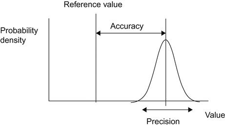
Accuracy and precision are the two terms in metrology that are most frequently mixed up or used indistinguishably. The accuracy of a measuring instrument indicates how close the result is to the true value. The precision of a measuring instrument refers to the dispersion of the results when making repeated measurements (sometimes referred to as repeatability). Figure 2.8 illustrates the difference between accuracy and precision. It is, therefore, possible to have a measurement that is highly precise (repeatable) but is not close to the true value that is inaccurate. This highlights the fundamental difference between the two terms and one must be careful when using them. Accuracy is a term relating the mean of a set of repeat measurements to the true value, whilst precision is representative of the spread of the measurements. Note that accuracy is rarely used as a quantitative value – it is more of a qualitative term. When it is necessary to use a quantitative measure of accuracy associated with a measurement, the measurement uncertainty should be used.
The VIM definition of accuracy is:
closeness of agreement between a measured quantity value and a true quantity value of a measurand.
and the definition of precision is:
closeness of agreement between indications or measured quantity values obtained by replicate measurements on the same or similar objects under specified conditions.
2.8.2 Resolution and error
The resolution of a measuring instrument is a quantitative expression of the ability of an indicating device to distinguish meaningfully between closely adjacent values of the quantity indicated. For example, for a simple dial indicator read by eye, the resolution is commonly given as half the distance between smallest, distinguishable indicating marks. It is not always either easy or obvious how to determine the resolution of an instrument. Consider for example an optical instrument that is used to measure surface texture and focuses light onto the surface. The lateral resolution is sometimes quoted in terms of the Rayleigh or Abbe criteria [29] although, depending on the numerical aperture of the focusing optics, the lateral resolution may be determined by the detector pixel spacing (see Section 6.7.1). The axial resolution will be a complex function of the optics, the detector electronics, the detection algorithm and the noise floor. This example highlights that resolution is not always a simple parameter to determine for a given instrument.
It is also important to note that one should always consider resolution hand in hand with other instrument performance indicators, such as accuracy and precision. Again, using the example of the optical surface measuring instrument, some surfaces can cause the instrument to produce errors that can be several hundred nanometres in magnitude, despite the fact that the instrument has an axial resolution of perhaps less than a nanometre (see Section 6.7.1).
The error in a measuring instrument is the difference between the indicated value and the true value (or the calibrated value of a transfer artefact). Errors usually fall into two categories depending on their origin. Random errors give rise to random fluctuations in the measured value and are commonly caused by environmental conditions, for example seismic noise or electrical interference. Systematic errors give rise to a constant difference from the true value, for example due to alignment error or because an instrument has not been calibrated correctly. Most measurements contain elements of both types of error, and there are different methods for either correcting errors or accounting for them in uncertainty analyses (see Ref. [30] for a more thorough discussion on errors). Also, errors can appear as random or systematic dependent on how they are treated.
The VIM definition of resolution is:
smallest change in a quantity being measured that causes a perceptible change in the corresponding indication.
and the definition of error is:
measured quantity value minus a reference quantity value.
2.8.3 Uncertainty in measurement
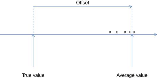
As discussed in the introductory text of Section 2.8, all measurements are imperfect. It follows that a measured value can be expected to differ from the true quantity value, and measured values obtained from repeated measurement to be dispersed about the true quantity value or some value offset from the true quantity value (Figure 2.9). A statement of uncertainty describes quantitatively the quality of a measured value as an estimate of the true quantity value.
A basic introduction to uncertainty of measurement is given elsewhere [31], although some of the more important terms and definitions are described briefly here. The Guide to the Expression of Uncertainty in Measurement (GUM) [32] is the definitive text on most aspects of uncertainty evaluation and should be read before the reader attempts an uncertainty evaluation for a particular measurement problem. A working group of the Joint Committee for Guides in Metrology (JCGM), the body responsible for maintaining the GUM and the VIM, is in the process of preparing a number of documents to support and extend the application of the GUM [33], and the following documents have been published by the working group:
• JCGM 101: 2008 on the propagation of distributions using a Monte Carlo method [34];
• JCGM 102: 2011 on extensions to any number of output quantities [35];
• JCGM 104: 2009 giving an introduction to the GUM and related documents [36]; and
• JCGM 106: 2012 on the role of measurement uncertainty in conformity assessment [37].
Additionally, the working group is in the process of revising the GUM itself [38].
The VIM definition of measurement uncertainty is:
non-negative parameter characterizing the dispersion of the quantity values being attributed to a measurand, based on the information used.
When measurement uncertainty is evaluated and reported as a coverage interval corresponding to a specified coverage probability p, it indicates an interval that contains the true quantity value with probability p.
2.8.3.1 The propagation of probability distributions
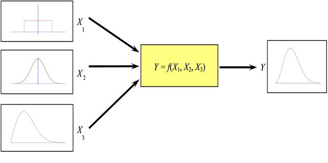
The basis for the evaluation of measurement uncertainty is the propagation of probability distributions (Figure 2.10). In order to apply the propagation of probability distributions, a measurement model of the generic form
(2.2)
relating input quantities X1, …, XN, about which information is available, and the measurand or output quantity Y, about which information is required, is formulated.
The input quantities include all quantities that affect or influence the measurement, including effects associated with the measuring instrument (such as bias, wear, drift), those associated with the artefact being measured (such as its stability), those associated with the measurement procedure, and ‘imported’ effects (such as the calibration of the instrument, material properties).
Information concerning the input quantities is encoded as probability distributions for those quantities, such as rectangular (uniform), Gaussian (normal). The information can take a variety of forms, including a series of indication values, data on a calibration certificate and the expert knowledge of the metrologist. An implementation of the propagation of probability distributions provides a probability distribution for Y, from which can be obtained an estimate of Y, the standard uncertainty associated with the estimate, and a coverage interval for Y corresponding to a stipulated (coverage) probability. Particular implementations of the approach are the GUM uncertainty framework (Section 2.8.3.2) and a Monte Carlo method (Section 2.8.3.3).
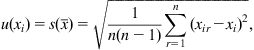
In a Type A evaluation of uncertainty, the information about an input quantity Xi takes the form of a series of indication values xir, r=1, …, n, obtained independently. An estimate xi of Xi is given by the average of the indication values, that is
(2.3)
with associated standard uncertainty u(xi) given by the standard deviation associated with the average, that is
(2.4)
 (2.4)
(2.4)
and degrees of freedom νi=n−1.
In a Type B evaluation of uncertainty, the information about Xi takes some other form and is used as the basis of establishing a probability distribution for Xi in terms of which an estimate xi and the associated standard uncertainty u(xi) are determined. An example is when the information about Xi is that Xi takes values between known limits a and b (a≤b). Then, Xi is characterised by a rectangular distribution on the interval [a, b], and xi and u(xi) are the expectation and standard deviation of Xi evaluated in terms of this distribution, that is
(2.5)
Note that there are other types of distribution, for example triangular and U-shaped, which are used to reflect different information about Xi.
2.8.3.2 The GUM uncertainty framework
The primary guide in metrology on uncertainty evaluation is the GUM [32]. It presents a framework for uncertainty evaluation based on the use of the law of propagation of uncertainty and the central limit theorem. The law of propagation of uncertainty provides a means for propagating uncertainties through the measurement model, that is for evaluating the standard uncertainty u(y) associated with an estimate y of Y given the standard uncertainties u(xi) associated with the estimates xi of Xi (and, when they are non-zero, the covariances u(xi, xj) associated with pairs of estimates xi and xj). The central limit theorem is applied to characterise Y by a Gaussian distribution (or, in the case of finite effective degrees of freedom, by a scaled and shifted t-distribution), which is used as the basis of providing a coverage interval for Y.
In the GUM uncertainty framework, the information about an input quantity Xi takes the form of an estimate xi, a standard uncertainty u(xi) associated with the estimate, and the degrees of freedom νi attached to the standard uncertainty.
The estimate y of the output quantity is determined by evaluating the model for the estimates of the input quantity, that is
(2.6)
The standard uncertainty u(y) associated with y is determined by propagating the standard uncertainties u(xi) associated with the xi through a linear approximation to the model. Writing the first-order Taylor series approximation to the model as
(2.7)
where ci is the derivative of first order of f with respect to Xi evaluated at the estimates of the input quantities, and assuming the Xi are uncorrelated, u(y) is determined from
(2.8)
In Eq. (2.8), which constitutes the law of propagation of uncertainty for uncorrelated quantities, the ci are called (first-order) sensitivity coefficients. A generalisation of the formula applies when the model input quantities are correlated.
An effective degrees of freedom νeff attached to the standard uncertainty u(y) is determined using the Welch–Satterthwaite formula, that is
(2.9)
The basis for evaluating a coverage interval for Y is to use the central limit theorem to characterise the random variable
(2.10)
by the standard Gaussian distribution in the case that νeff is infinite or a t-distribution otherwise. A coverage interval for Y corresponding to the coverage probability p takes the form
(2.11)
U is called the expanded uncertainty given by
(2.12)
where k is called a coverage factor, and is such that
(2.13)
where Z is characterised by the standard Gaussian distribution in the case that νeff is infinite or a t-distribution otherwise.
There are some practical issues that arise in the application of the GUM uncertainty framework. Firstly, although the GUM uncertainty framework can be expected to work well in many circumstances, it is generally difficult to quantify the effects of the approximations involved, which include linearisation of the model in the application of the law of propagation of uncertainty, the evaluation of effective degrees of freedom using the Welch–Satterthwaite formula and the assumption that the output quantity is characterised by a Gaussian or (scaled and shifted) t-distribution. Secondly, the procedure relies on the calculation of the model sensitivity coefficients ci as the basis of the linearisation of the model. Calculation of the ci can be difficult when (i) the model is (algebraically) complicated or (ii) the model is specified as a numerical procedure for calculating a value of Y, for example as the solution to a differential equation.
2.8.3.3 A Monte Carlo method
A Monte Carlo method for uncertainty evaluation is based on the following consideration. The estimate y of Y is conventionally obtained, as in the previous section, by evaluating the model for the estimates xi of Xi. However, since each Xi is described by a probability distribution, a value as legitimate as xi can be obtained by drawing a value at random from the distribution. The method operates, therefore, in the following manner. A random draw is made from the probability distribution for each Xi and the corresponding value of Y is formed by evaluating the model for these values. Many Monte Carlo trials are performed, that is the process is repeated many times, to obtain M, say, values yr, r=1, …, M, of Y. Finally, the values yr are used to provide an approximation to the probability distribution for Y.
An estimate y of Y is determined as the average of the values yr of Y, that is
(2.14)
The standard uncertainty u(y) associated with y is determined as the standard deviation of the values yr of Y, that is
(2.15)
A coverage interval corresponding to coverage probability p is an interval [ylow, yhigh] that contains 100p% of the values yr of Y. Such an interval is not uniquely defined. However, two particular intervals are of interest. The first is the probabilistically symmetric coverage interval for which 100(1−p)/2% of the values are less than ylow and the same number are greater than yhigh. The second is the shortest coverage interval, which is the shortest of all intervals containing 100p% of the values.
The Monte Carlo method has a number of features, including (i) that it is applicable regardless of the nature of the model, that is whether it is linear, mildly non-linear or highly non-linear, (ii) that there is no requirement to evaluate effective degrees of freedom and (iii) that no assumption is made about the distribution for Y, for example that it is Gaussian. In consequence, the method provides results that are free of the approximations involved in applying the GUM uncertainty framework, and it can be expected, therefore, to provide an uncertainty evaluation that is reliable for a wide range of measurement problems. Additionally, the method does not require the calculation of model sensitivity coefficients since the only interaction with the model is to evaluate the model for values of the input quantities.
However, there are also some practical issues that arise in the application of a Monte Carlo method. The degree of numerical approximation obtained for the distribution for Y is controlled by the number M of trials, and a large value of M (perhaps 105 or 106 or even greater) may sometimes be required. One issue, therefore, is that the calculation for large values of M may not be practicable, particularly when a (single) model evaluation takes an appreciable amount of time. Another issue is that the ability to make random draws from the probability distributions for the Xi is central, and the use of high-quality algorithms for random-number generation gives confidence that reliable results are provided by an implementation of the method. In this regard, the ability to draw pseudo-random numbers from a rectangular distribution is fundamental in its own right, and also as the basis for making random draws from other distributions using appropriate algorithms or formulae.
2.9 The laser
The invention of the laser in 1960 has had a significant impact on metrology. The realisation of the definition of the metre (see Section 2.3) involves the use of a frequency-stabilised laser, and many commercial interferometer systems use a laser source. The most common form of laser in the metrology area is the helium–neon laser, although solid-state lasers are becoming more widespread.
2.9.1 Theory of the helium–neon laser
The tube of a continuous-wave helium–neon (He–Ne) gas laser contains a mixture of approximately eight parts of helium to one part of neon at a total pressure of a few millibars. The laser consists of an optical cavity, similar to that of a Fabry–Pérot etalon (see Section 4.4.4), formed by a plasma tube with optical-quality mirrors (one of which is semi-transparent) at both ends. The gas in the tube is excited by a high-voltage discharge of approximately 1.5–2.5 kV, at a current of approximately 5–6 mA. The discharge creates a plasma in the tube that emits radiation at various wavelengths corresponding to the multitude of allowed transitions in the helium and neon atoms.
The coherent radiation emitted by the He–Ne laser at approximately 632.8 nm wavelength corresponds to the 3s2–2p4 atomic transition in neon [39]. The excited 3s2 level is pumped by energetic 2s0 helium atoms colliding with the neon atoms; the 2s0 helium energy level is similar in energy to the 3s2 level of neon, and the lighter helium atoms are easily excited into the 2s0 level by the plasma discharge (Figure 2.11). The excess energy of the collision is approximately thermal, that is it is easily removed by the atoms in the plasma as kinetic energy.

The collisional pumping of the 3s2 level in neon produces the selective excitation, or population inversion, that is required for lasing action. The 2p neon state decays in 10−8 seconds to the 1s state, maintaining the population inversion. This state relaxes to the ground state by collision with the walls of the plasma tube. The laser gain is relatively small and so losses at the end of the mirrors must be minimised by using a high-reflectance coating, typically 99.9%. The output power is limited by the fact that the upper lasing state reaches saturation at quite low discharge powers, whereas the lower state increases its population more slowly. After a certain discharge power is reached, further increase in the power leads to a decrease in the population inversion, and hence lower light power output.
The 632.8 nm operating wavelength is selected by the spacing of the end mirrors, that is by the total length of the optical cavity, lc. The length of the cavity must be such that the waves reflected by the two end mirrors are in phase for stimulated emission to occur. The wavelengths of successive axial modes are then given by
(2.16)
These modes are separated in wavenumber by
(2.17)
or in terms of frequency
(2.18)
where c is the speed of light in a vacuum. This would lead to a series of narrow lines of similar intensity in the spectrum, if it were not for the effects of Doppler broadening and the Gaussian distribution of atoms available for stimulated emission.
When a particular mode is oscillating, there is a selective depopulation of atoms with specific velocities (laser cooling) that leads to a dip in the gain profile. For modes oscillating away from the centre of the gain curve, the atomic populations for the two opposite directions of propagation are different due to the equal but opposite velocities. For modes oscillating at the centre of the gain curve, the two populations become a single population of effectively stationary atoms. Thus, a dip in the gain profile occurs at the centre of the gain curve – the so-called Lamb dip. The position of the Lamb dip is dependent on other parameters of the laser such as the position of the gain curve and can be unstable.
For early lasers with typical cavity lengths of 1 m, the mode spacing was 0.5 m−1, with a gain profile width of approximately 5.5 m−1. Thus, several axial modes were present in the gain profile with gains sufficient for laser action, and so two or more modes would operate simultaneously, making the laser unsuitable for coherent interferometry. By using a shorter tube and then carefully lowering the power of the discharge, and hence lowering the gain curve, it is possible to achieve single-mode operation.
2.9.2 Single-mode laser wavelength stabilisation schemes
To allow a laser to be used in interferometry with coherence lengths above a few millimetres (see Section 4.3.4), it must operate in a single mode and there have been many proposed schemes for laser stabilisation.
The Lamb dip, mentioned above, was used in an early stabilisation scheme. Here the intensity of the output beam was monitored as the length of the cavity was modulated, for example by piezoelectric actuators (PZTs). Alternatively, mirrors external to the laser cavity are used that could be modulated – the output intensity being monitored and the laser locked to the centre of the Lamb dip. The reproducibility of lasers locked to the Lamb dip is limited by shift of the Lamb dip centre as the pressure of the gas inside the laser tube varies and by a discharge current-dependent shift. The large width of the Lamb dip itself (about 5×10⁻⁷ of the laser frequency) also limits the frequency stability obtainable from this technique.
Use has also been made of tuneable Fabry–Pérot etalons in a similar system. Other groups have locked the output of one laser to the frequency of a second stabilised laser. Others have used neon discharge absorption cells, where the laser was locked to the absorption spectrum of neon in an external tube, the theory being that the unexcited neon would have a narrower linewidth than the neon in the laser discharge.
2.9.3 Laser frequency stabilisation using saturated absorption
The technique with the greatest stability is used in the Primary Reference lasers which realise a typical NMI’s Primary Standard of Length and involves controlling the length of the laser cavity to alter the wavelength and locking the wavelength to an absorption line in saturated iodine vapour [40]. This is a very stable technique since the absorption takes place from a thermally populated energy level that is free from the perturbing effects of the electric discharge in the laser tube.
If the output beam from a laser is passed straight through an absorption cell, then absorption takes place over a Doppler-broadened transition. However, if the cell is placed in a standing-wave optical field, the high-intensity laser field saturates the absorption and a narrow dip appears at the centre of the absorption line corresponding to molecules that are stationary or moving perpendicular to the direction of beam propagation. This dip produces an increase in the laser power in the region of the absorption line. The absorption line is reproducible and insensitive to perturbations. The linewidth is dependent on the absorber pressure, laser power and energy level lifetime. Saturated absorption linewidths are typically less than 1×10⁻⁸ of the laser wavelength.
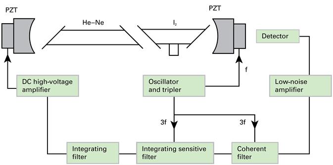
In a practical application, an evacuated quartz cell containing a small iodine crystal is placed in the laser cavity and temperature controlled to 15°C. As the iodine partly solidifies at this temperature, this guarantees a constant iodine gas pressure. The laser mirrors are mounted on PZTs and the end plates are separated by low thermal expansion bars to ensure a thermally stable cavity. A small frequency modulation is then applied to one of the PZTs. This leads to an amplitude modulation in the output power that is detected using a phase-sensitive detector and fed back to the other PZT as a correction signal. The frequency control system employs a photodiode, low-noise amplifier, coherent filter and phase-sensitive detector followed by an integrating filter. Figure 2.12 is a schema of the iodine-stabilised He–Ne instrumentation.
Detection of the absorption signal at the laser modulation frequency results in a first derivative scan that shows the hyperfine components superimposed on the sloping background of the neon gain curve. The laser may be servo-locked to any of these lines, the frequency of which has been fixed (together with their uncertainties) internationally at the time of the redefinition of the metre in 1983 in terms of the speed of light, and which has been fine-tuned a few times since then.
Iodine-stabilised He–Ne lasers can achieve frequency stability of a few parts in 1013 over a period of a few minutes with long-term reproducibility of a few parts in 1011. The reproducibility of iodine-stabilised He–Ne lasers, when being operated under certain conditions, enables the independent manufacture of a primary length standard without a need to refer or compare to some other standard. Contrary to this concept, NMIs compare their reference standards with each other to ensure that no unforeseen errors are being introduced. Until recently, these comparisons were commonly made at the BIPM, similar to when the metre bars were in use [40].
2.9.3.1 Two-mode stabilisation
Instead of emitting one frequency, a laser can be designed in such a way that it radiates in two limited frequency regions. Figure 2.13 shows this schematically. If two (longitudinal) modes exist, then both should be orthogonally linearly polarised.

As the laser cavity length changes, the modes move through the gain curve, changing in both frequency and amplitude. The two modes are separated into two beams by polarisation components, and their amplitudes are compared electronically. The cavity length is then adjusted, usually by heating a coil around the laser tube that is kept at approximately 40°C, to maintain the proper relationship between the modes. By using a polariser, only one beam is allowed to exit the system. Such lasers are commonly used in homodyne interferometry (see Section 5.2.2).
In the comparison method of stabilisation, the ratio of the intensities of the two orthogonal beams is measured and is kept constant. This ratio is independent of output power and accurately determines the output frequency of the beam. In the long term, the frequency may shift due to variations in the He–Ne gas pressure and ratio. By adjusting the intensity ratio, the output frequency can be swept by approximately 300 MHz, while maintaining a 1 MHz linewidth.
In the slope method of stabilisation, only the intensity of the output beam is monitored, and a feedback loop adjusts the cavity length to maintain constant power. Because of the steep slope of the laser gain curve, variations in frequency cause an immediate and significant change in output power. The comparison method is somewhat more stable than the slope method, since it measures the amplitude of the two modes and centres them accurately around the peak of the gain curve, which is essentially an invariant, at least in the short term, and the frequency is unaffected by long-term power drift caused by ageing or other factors. On the other hand, the slope method of frequency control significantly simplifies the control electronics. Another stabilising method is stabilising the frequency difference, as the frequency difference appears to have a minimum when the intensities are equal.
2.9.4 Zeeman-stabilised 633 nm lasers
An alternative technique to saturated absorption is used in many commercial laser interferometers. The method of stabilisation is based on the Zeeman effect [41,42]. A longitudinal magnetic field is applied to a single-mode He–Ne laser tube, splitting the normally linearly polarised mode into two counter-rotating circular polarisations. A field strength of 0.2 T is sufficient to split the modes, which remain locked together at low magnetic field, to produce the linear polarisation. These two modes differ in frequency by typically 3 MHz, around a mean frequency corresponding to the original linear mode [43].
The wavelength difference between the two modes is due to each of the two modes experiencing a different refractive index and, therefore, different optical path length, in the He–Ne mixture. This arises due to magnetic splitting of an atomic state of neon, shown in Figure 2.14.
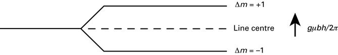
The Δm=+1 mode couples with the left polarised mode and the Δm=−1 mode couples with the right polarised mode. The relative frequencies of the polarisation modes are given by
(2.19)
where L is the cavity length, n is the refractive index for the mode and N is the axial quantum number [44].
The important feature of the Zeeman split gain curve is that the position of ω0 does not vary with magnetic field strength – it remains locked at the original (un-split) line centre, and thus a very stable lock point. If one combines the two oppositely polarised components, one observes a heterodyne beat frequency between them given by
(2.20)
which is proportional to ![]() , where χ+(n) and χ−(n) are dispersion functions for the left and right polarised modes, respectively. For a more complete derivation see Ref. [45]. As the laser is tuned by altering the cavity length, L, the beat frequency will pass through a peak that corresponds to the laser frequency being tuned to ω0.
, where χ+(n) and χ−(n) are dispersion functions for the left and right polarised modes, respectively. For a more complete derivation see Ref. [45]. As the laser is tuned by altering the cavity length, L, the beat frequency will pass through a peak that corresponds to the laser frequency being tuned to ω0.
This tuning curve can be used as an error signal for controlling the laser frequency. The particular method used to modulate the laser cavity is usually thermal expansion. A thin foil heater is attached to the laser tube and connected to a square-root power amplifier. Two magnets are fixed onto the tube to provide the axial magnetic field. A polarising beam splitter is used, together with a photodetector and amplifier to detect the beat frequency. This error signal is fed to various stages of counters and amplifiers and then to the heater.
The laser tube requires a period of approximately 10 min to reach the correct temperature corresponding to the required tube length for operation at frequency, ω0. A phase-locked loop circuit then fine-tunes the temperature, and consequently the length of the cavity, to stabilise the laser at the correct frequency. This last process takes only a few seconds to achieve lock. The frequency stability of the laser is 5×10⁻¹⁰ for 1 s averages and is white-noise limited for averaging times between 100 ms and 10 min. The day-to-day reproducibility of the laser frequency is typically ±5×10⁻¹⁰. There is also a linear drift of frequency with the total amount of time for which the laser has been in operation. This is due to clean-up of the helium–neon mixture whilst undergoing discharge. The rate of drift is unique to each laser, but is stable with respect to time, and can be ascertained after a few calibrations of the laser frequency. As an example, Tomlinson and Fork [46] showed drift rates of 0.3–5.7 MHz ±0.5 MHz per calendar year, although these were for frequency against date, rather than against operational time. Rowley [45] reported a drift rate of −1×10⁻¹¹ per hour of operation.
An attractive feature of the Zeeman-stabilised laser is that the difference in amplitude can be used for stabilisation, and the difference in frequency can be taken as the reference signal when it is used in heterodyne displacement interferometry (see Section 5.2.3).
2.9.5 Frequency calibration of a (stabilised) 633 nm laser
The calibration of a laser’s frequency is achieved by combining the light from the stabilised laser with a primary (reference) laser via a beam splitter. The beat signal between the two frequencies is measured with a photodetector (Figure 2.15). If the beams are carefully aligned, the beams interfere and the interference intensity varies in time with the frequency difference (see Section 4.3.2 and Eq. (4.5)). If the laser frequencies are close enough, this beat frequency can be detected electronically and monitored over a number of hours. Typical values of the beat signal range between 50 and 500 MHz, with the iodine standard stabilised on one of its dips. As the reference laser, if it is an iodine-stabilised laser, is continuously swept over some 6 MHz, it is common to integrate the frequency difference over 10 s. If the reference beam is generated by a frequency comb [47], the reference laser is not continuously swept and the integration time can be shorter, representing the time in which laser interferometers are taking measurements.

As a beat frequency is an absolute value, the reference laser needs to be stabilised on different frequencies in order to determine whether the frequency of the calibrated laser is higher or lower than the reference frequency. A Zeeman-stabilised laser emits two polarisations that are separated, typically by 3 MHz. During laser calibrations, beats between each of these frequencies and the iodine frequency are measured. The mean of these can be considered to be the calibrated wavelength of the Zeeman-stabilised laser under test if the difference is within the uncertainty limits. Also, it is common to measure just one frequency and to take the other into account in the uncertainty; 3 MHz corresponds to a relative uncertainty of about 6×10⁻⁹ in frequency and so in a measured length.
If the two modes of a two-mode laser are used in the same manner, as in a common Zeeman-based laser interferometer system, then the two polarisations may differ by up to 1 GHz, which corresponds to 2×10⁻⁶. However, it is more common that one of the beams is blocked by a polariser and the system is used as a homodyne interferometer (see Section 5.2.2). In this case, a single frequency should be measured.
2.9.6 Modern and future laser frequency standards
As mentioned in Section 2.3, the current definition of length is based on a fixed speed of light, and there are a number of recipes to make an optical wavelength/frequency standard. These optical standards are linked to the time standard (which is a microwave standard) via a series of relatively complicated comparisons to determine an absolute frequency and an uncertainty.
The most direct generation of an optical wavelength that is linked to a radio frequency standard, such as an atomic clock, is the so-called frequency comb [47]. A frequency comb generates a series of equally spaced (the ‘comb’) frequencies by linking a nanosecond pulsed laser to an atomic clock. This makes a direct comparison possible of optical frequencies to the time standard without the need for an intermediate (still primary) standard such as the iodine-stabilised laser.
The development of frequency combs is an important breakthrough as, along with the He–Ne-based gas lasers, ranges of solid-state lasers and diode lasers have become available as frequency-stabilised light sources. These can have wavelengths that are very different from the common He–Ne wavelengths (e.g. the red 633 nm wavelength), and cannot be measured using a beat measurement with a He–Ne laser, because the beat frequency is too high to be measured directly. Frequency combs also further enable the development of other stabilised laser systems, such as stabilised diode lasers. Diode lasers can have a far wider wavelength range than He–Ne gas lasers and can, for example, be used in the swept-frequency absolute distance interferometry, as described in Section 5.2.7.
On the one hand, the frequency comb takes away the necessity of an iodine-stabilised laser as an essential step in establishing traceable measurements in length metrology; on the other hand, the iodine-stabilised reference standard can be calibrated using a frequency comb, making it a transfer standard rather than a primary standard; however, with an even smaller uncertainty, as the calibration may correct for small offsets that are incorporated in the uncertainty in the definition as a primary standard.
Direct use of frequency combs has been explored, where applications are found in highly accurate long-distance measurements, achieving 1.1 µm uncertainty over 50 m [48,49], increasing the range and resolution for small displacement measurements, and achieving 24 pm resolution over 14 µm displacement [50]. Also, direct application in gauge block measurement has been explored (see Chapter 4), as well as simultaneous measurement of the thickness and refractive index (and dispersion) of flat samples [51].
Because of the complexity and expenses of frequency combs, they will not easily find their way outside of specialised laboratories, but the frequency comb technology will open more ways to directly traceable measurements of long sizes and distances in the future.