
Precision Measurement Instrumentation – Some Design Principles
Richard Leach
This chapter introduces many of the concepts necessary for the precision design of measuring instruments. The geometry of the various structural elements of an instrument is discussed along with principles of symmetry. Kinematic design is covered in detail along with examples of fully constrained systems (the Kelvin clamps) and controlled degree of freedom motion devices. Motion and dynamics are addressed and the Abbe principle is covered in detail. Elastic compression and the different forms of force loop on an instrument (structural, thermal and metrological) are discussed along with methods to minimise the effects of thermal and mechanical error sources. Lastly, vibration isolation is covered in detail.
Keywords
Precision Engineering; Geometry; Kinematic Design; Constraints; Elastic Averaging; Degree of Freedom; Kelvin Clamps; Motion; Dynamics; Abbe Principle; Elastic Compression; Force Loops; Vibration Isolation
The design, development and use of precision measurement instrumentation1 is a highly specialised field that combines precision engineering with metrology. Although precision instrumentation has been around for many decades (see Ref. [1] for a historical overview), the measurements that are required to support micro- and nanotechnology (MNT) have forced designers and metrologists to learn a number of new skills. One major difference between conventional-scale instrumentation and that used to measure MNT structures and devices is the effect that the measuring instrument has on the measurement process. For example, when measuring surface topography with a stylus instrument (see Section 6.6.1), one should be aware of the possible distortion of the topography caused by the finite shape of the stylus. In essence, the business end of the instrument can have a size that is comparable to the structure being measured. This ‘probe–measurand’ interaction will be discussed throughout this book where necessary for each type of instrument. This chapter will present the basic principles of precision instrumentation so that, as the reader is presented with the various instruments in the following chapters, he or she will be armed with the appropriate knowledge to understand the basic operating principles.
Precision instrument design involves scientific disciplines such as mechanics, materials, optics, electronics, control, thermomechanics, dynamics and software engineering. Introductions to many of the precision design and metrology concepts discussed in this chapter are given elsewhere [2–5]. The rest of the chapter follows the design considerations of Ref. [6] and is by no means exhaustive.
3.1 Geometrical considerations
Most precision measuring instrument designs involve parts that are formed from simple geometrical elements such as cubes, cylinders, tubes, beams, spheres and boxes to support loads in the system. Surfaces that are used for moving elements are often formed from flats and cylinders. In practice, however, deviations from these ideal shapes and structures occur due to form and surface texture error caused by the machining processes used to manufacture the parts. The environment in which an instrument is housed also affects geometry, for example vibration, temperature gradients and ageing can cause undesirable dimensional changes.
Other factors that can affect the geometry of an instrument include the effects of the connections between different parts, loading of the structure by the weight of the parts, stiffness and other material properties. The above deviations from ideal geometry cause the various parts that make up an instrument to interact in a way that is very difficult to predict in practice. Also, to reiterate the point made in the previous section, of great importance on the MNT scale is the effect of the measuring probe on the part being measured and the measuring result.
3.2 Kinematic design
James Clark Maxwell (1890) was one of the first scientists to rigorously consider kinematic design. He stated that:
The pieces of our instruments are solid, but not rigid. If a solid piece is constrained in more than six ways it will be subject to internal stress, and will become strained or distorted, and this in a manner which, without the most micromechanical measurements, it would be impossible to specify.
These sentences capture, essentially, the main concepts of kinematic design. Kinematics is a branch of mechanics that deals with relationships between the position, velocity and acceleration of a body. Kinematic design aims to impart the required movements on a body by means of constraints [3,7]. Also, kinetics is the study of the forces involved in motion and often forms part of kinematic design. The principle aim of kinematic design is to allow assembly of components with a minimal amount of strain and/or to allow maximum repeatable relocation.
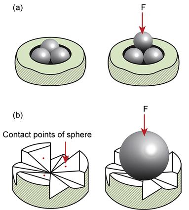
A rigid body possesses six degrees of freedom in motion – three linear and three rotational. In Cartesian coordinates, the degrees of freedom are in the x-, y- and z-directions plus rotations about each of the axes. A constraint is that which prevents minimally motion in just one of the degrees of freedom. Typically a constraint will be a point contact (at least approximately), for example a ball on a flat (Figure 3.1). Assuming the ball is rigid, the point contact will constrain one degree of freedom and, if held by a force (see Figure 3.1), introduces one constraint. Note that two contact points are required to prevent motion in a rotational degree of freedom.

There are two lemmas of kinematic design [3]:
1. any unconstrained rigid body has six degrees of freedom;
2. the number of contact points between any two perfectly rigid bodies is equal to the number of constraints.
This means that
Note that pure kinematic design is often impractical due to the loads involved, manufacturing costs, materials available and other factors. Whereas, over-constraint (more than six constraints) will introduce unwanted strain and should generally be avoided, in practical situations a high degree of over-constraint (many contact points for one constraint) is applied to average out the forces on a system – this is known as elastic averaging. An example of elastic averaging (also referred to as semi-kinematic design) is the use of a sphere in a cone, rather than a trihedral recess (see Section 3.2.1). A cone is easy to manufacture and has a higher load-bearing capacity than the trihedral hole. Under-constraint (less than the required number of constraints) will result in unwanted motion and should be avoided.
There are often many assumptions applied when carrying out kinematic design. Real bodies are not perfectly rigid and will experience both elastic and possibly plastic deformations under a load. Such deformations will exclude perfect point contacts and cause unwanted motions. For this reason, it is often important to choose with care the materials, shapes and surface texture of a given part. Despite this, kinematic design is an extremely important concept that the precision instrument designer must master. Two examples of kinematic design will be considered here – the Kelvin clamp and a single degree of freedom motion system. Note that kinematic design should be used with discretion – kinematics implies that a chair should have three legs, but safety implies that four is better (a degree of leg flexure is tolerated).
3.2.1 The Kelvin clamps
Type I and Type II Kelvin clamps are examples of fully constrained systems, that is ones with six constraints. When designed properly, these clamps are very effective where accurate re-positioning is required and can be stable to within nanometres [8], although around 0.1 µm is more usual.
Both clamps have a top plate (on which, for example, the object to be measured is placed) that has three rigid spheres (or hemispheres) spaced on a diameter. The three spheres then contact on a flat and in a vee and a trihedral hole, as in Figure 3.2(a), or in three vee-grooves, as in Figure 3.2(b). In the Type II clamp, it is easy to see where the six points of contact, that is constraints are – two in each vee-groove. In the Type I clamp, one contact point is on the flat, two more are in the vee-groove and the final three are in the trihedral hole. The Type I clamp has the advantage of a well-defined translational location based on the position of the trihedral hole, but it is more difficult to manufacture. A trihedral hole can be produced using an angled vee-shaped milling cutter (Figure 3.3(b)) or by pressing three spheres together in a flat-bottomed hole – the contacting spheres will then touch at a common tangent (see Figure 3.3(a)). For miniature structures, an anisotropic etchant can be used on a single crystalline material [9]. The Type II clamp is more symmetrical and less influenced by thermal variations. Note that the symmetrical groove pattern confers its own advantages (symmetry) but is not a kinematic requirement; any set of grooves will do, provided that they are not all parallel.

3.2.2 A single degree of freedom motion device
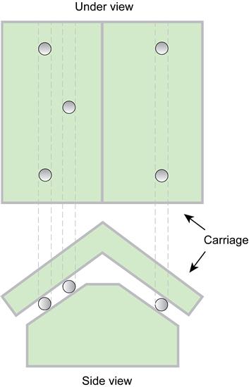
There are many methods for producing single degree of freedom motion (see, for example, Ref. [10]). One method that directly uses the idea of single point contacts is the prismatic slideway [3]. The contact points are distributed on two non-parallel flat surfaces as shown in Figure 3.4. In practice, the spheres would be attached to the carriage (and would usually be just parts of a sphere to give a point contact). The degrees of freedom in the system can be deduced by considering the loading necessary to keep all five spheres in contact. Firstly, the three-point support could be positioned onto the horizontal plane, resulting in a linear constraint in the z-axis and rotary constraints about the x- and y-axes. A carriage placed on this plane is free to slide in the x-direction until either of the two remaining spheres contacts the vertical face. The x-axis linear degree of freedom is then constrained. Further horizontal force would cause the carriage to rotate until the fifth sphere comes into contact, removing the rotary degree of freedom about the z-axis. This gives a single degree of freedom linear motion along the y-axis.
3.3 Dynamics
Most precision instruments used for MNT metrology involve some form of moving part. This is especially true of surface texture measuring instruments and coordinate measuring machines (CMMs). Motion usually requires some form of guideway, this being two or more elements that move relative to each other with fixed degrees of freedom. For accurate positioning, the play and the friction between the parts in the guideway must be reduced (unless the friction characteristics are being used to impart damping on the guideway). To avoid sticking and slipping of the guideway, the friction should normally be minimised and kept at a constant value even when there are velocity or acceleration changes. It is also important that a guideway has a smooth motion profile to avoid high accelerations and forces.
The symmetry of a dynamic system plays an important role. With a rotating part, the unbalance and mass moment of inertia must be reduced. A linear guideway should be driven through an axis that minimises any angular motion in its travel (its axis of reaction). The centres of friction and inertia should be kept on the line of the drive axis. Stiffness is another important factor; there must be a trade-off between minimising the forces on a guideway and maximising its transverse stiffness. As with the metrology frame (see Section 3.6), the environment in which the instrument is housed affects its dynamic characteristics.
Guideways can be produced using many techniques, but the most popular three are as follows:
1. flexures – usually used only over a small range owing to the elastic limit and parasitic motion [3,11,12];
2. dry or roller-bearing linear slideways – as used on surface profile measuring instruments, for example Ref. [13];
Many of the most advanced guideways use active feedback control systems [15,16].
3.4 The Abbe principle
The Abbe principle was first described by Ernst Abbe (1890) of Zeiss and states:
If errors of parallax are to be avoided, the measuring system must be placed co-axially (in line with) the line in which displacement (giving length) is to be measured on the work-piece.
Abbe error occurs when the measuring point of interest is displaced laterally from the actual measuring scale location (reference line or axis of measurement), and when angular errors exist in the positioning system. Abbe error causes the measured displacement to appear longer or shorter than the true position, depending on the angular offset. The spatial separation between the measured point and the reference line is known as the Abbe offset. Figure 3.5 shows the effect of Abbe error on an interferometric measurement of length. To ensure zero Abbe error, the reflector axis of movement should be co-linear with the axis of measurement. To account for the Abbe error in an uncertainty analysis relies on knowing the magnitude of the Abbe offset and the magnitude of the errors in motion of the positioning system (e.g. straightness).

The Abbe error is given by
where d is the Abbe offset and θ is the angular error of the scale motion.
The Abbe principle is, perhaps, the most important principle in precision instrument design and is also one that is commonly misunderstood – Bryan [17] described it as the first principle of machine design and dimensional metrology. Abbe’s original paper concentrated on one-dimensional measuring instruments. Bryan restated the Abbe principle for multidimensional systems as:
The displacement measuring system should be in line with the functional point whose displacement is to be measured. If this is not possible, either the slideways that transfer the displacement must be free of angular motion or angular motion data must be used to calculate the consequences of the offset.
Many three-axis instruments, especially CMMs, attempt to minimise the Abbe error through good design principles (see Chapter 8). Three good examples of this are the Zeiss F25 CMM [18], the ISARA CMM [19] and the Tri-Nano CMM [20].
3.5 Elastic compression
When any instrument uses mechanical contact, or when different parts of an instrument are in mechanical contact, there will be some form of compression due to any applied forces. This compression will mean that a point contact always involves some degrees of elastic averaging. With good design, such compression will be minimal and can be considered negligible, but when micrometre or nanometre tolerances or measurement uncertainties are required, elastic compression must be accounted for, either by making appropriate corrections or by taking account of the compression in an uncertainty analysis. In some cases, where the applied load is relatively high, irreversible, or plastic, deformation may occur. This is especially probable when using either high forces or small contact areas, for example when using stylus instruments (see Section 6.6.1) or atomic force microscopes (see Section 7.3). The theory behind elastic and plastic deformation can be found in detail elsewhere [21].
The amount that a body compresses under applied load depends on:
• the measurement force or applied load;
• the geometry of the bodies in contact;
• the material characteristics of the bodies in contact;
The formulae for calculating the amount of compression for most situations can be found in Ref. [21], and there are a number of calculators available on the Internet (see, for example, emtoolbox.nist.gov/Main/Main.asp). The most common cases will be included here. More examples of simple compression calculations are given elsewhere [4]. For a sphere in contact with a single plane (Figure 3.6), the mutual compression (i.e. the combined compression of the sphere and the plane) is given by
(3.1)
where D is the diameter of the sphere, P is the total applied force and V is defined as
(3.2)
where E is the Young’s modulus of the material and σ is the Poisson’s ratio. Note that the assignment of the subscript for the two materials is arbitrary due to the symmetry of the interaction. For a sphere between two parallel planes of similar material, Eq. (3.1) is modified by removing the factor of two in the denominator.

For a cylinder in contact with a plane, the compression is given by
(3.3)
where 2a is the length of the cylinder, and the force per unit length is given by
(3.4)
Plastic compression is much more complicated than elastic compression and will be highly dependent upon the types of materials and surfaces considered. Many examples of both elastic and plastic compression are considered in Ref. [22].
3.6 Force loops
There are three types of loop structures found on precision measuring instruments: structural loops, thermal loops and metrology loops. These three structures are often interrelated and can sometimes be indistinguishable from each other.
3.6.1 The structural loop
A structural loop is an assembly of mechanical components that maintain relative position between specified objects. Using a stylus surface texture measuring instrument as an example (see Section 6.6.1 and Figure 6.8), the structural loop runs along the base plate and up the bridge, through the probe, through the object being measured, down through the x-slideway and back into the base plate to close the loop. It is important that the separate components in the structural loop have high stiffness to avoid deformations under loading conditions – deformation in one component will lead to uncompensated dimensional change at the functional or measurement point.
3.6.2 The thermal loop
A thermal loop is described as a path across an assembly of mechanical components, which determines the relative position between specified objects under changing temperatures [6]. Much akin to mechanical deformations in the structural loop, temperature gradients across an instrument can cause thermal expansion and resulting dimensional changes. It is possible to compensate for thermal expansion by choosing appropriate component lengths and materials. If well designed, and if there are no temperature gradients present, it may just be necessary to make the separate components of an instrument from the same material. Thermal expansion can also be compensated by measuring thermal expansion coefficients and temperatures and applying appropriate corrections to measured lengths. This practice is common in gauge block metrology where the geometry of the blocks being measured is well known [23]. Obviously, the effect of a thermal loop can be minimised by controlling the temperature stability of the room, or enclosure, in which the instrument is housed.
3.6.3 The metrology loop
A metrology loop is a reference frame for displacement measurements, independent of the instrument base. In the case of many surface texture measuring instruments or CMMs, it is very similar to the structural loop. The metrology loop should be made as small as possible to avoid environmental effects. In the case of an optical instrument, relying on the wavelength of its source for length traceability, much of the metrology loop may be the air paths through which the beam travels. Fluctuations in the air temperature, barometric pressure, humidity and chemical composition of these air paths cause changes in the refractive index and corresponding changes to the wavelength of the light [24,25]. This can cause substantial dimensional errors. The last example demonstrates that the metrology and structural loops can be quite different.
3.7 Materials
Nearly all precision measuring instrument designs involve minimising the influence of mechanical and thermal inputs which vary with time and which cause distortion of the metrology frame. Exceptions to this statement are, of course, sensors and transducers designed to measure mechanical or thermal properties. There are three ways (or combinations of these ways) to minimise the effects of disturbing inputs:
1. isolate the instrument from the input, for example using thermal enclosures and anti-vibration tables;
2. use design principles and choose materials that minimise the effect of disturbing inputs, for example thermal compensation design methods, materials with low coefficients of expansion and stiff structures with high natural frequencies;
3. measure the effects of the disturbing influences and correct for them.
The choice of materials for precision measuring instruments is closely linked to the design of the force loops that make up the metrology frame.
3.7.1 Minimising thermal inputs
Thermal distortions will usually be a source of inaccuracy. To find a performance index for thermal distortion, consider a horizontal beam supported at both ends of length L and thickness h [26]. One face of the beam is exposed to a heat flux of intensity Q in the y-direction that sets up a temperature, T, gradient, dT/dy, across the beam. Assuming the period of the heat flux is greater than the thermal response time of the beam, then a steady state is reached with a temperature gradient given by
(3.5)
where λ is the thermal conductivity of the beam. The thermal strain is given by
(3.6)
where α is the thermal expansion coefficient and T0 is the ambient temperature. If the beam is unconstrained, any temperature gradient will create a strain gradient, dε/dy in the beam causing it to take up a constant curvature given by
(3.7)
Integrating along the beam gives the central deflection of
(3.8)
where C1 is a constant that depends on the thermal loads and the boundary conditions. Thus, for a given geometry and thermal input, the distortion is minimised by selecting materials with large values of the performance index
(3.9)
In Refs. [3,27], they arrive at the same index by considering other types of thermal load. If the assumption that the period of the heat flux is greater than the thermal response time of the beam is not valid, then the thermal mass of the beam has to be taken into account [27]. In this case, thermal conductivity is given by
(3.10)
where D is the thermal diffusivity of the beam material, ρ is its density and Cp is its specific heat capacity. In the case of a room with stable temperature and very slow heat cycling, Eq. (3.9) is normally valid.
3.7.2 Minimising mechanical inputs
There are many types of mechanical input that will cause unwanted deflections of a metrology frame. These include elastic deflections due to self-weight, loading due to the object being measured and external vibration sources. To minimise elastic deflections, a high stiffness is desirable. The elastic self-deflection of a beam is described by
(3.11)
where W is the weight of the beam, E is the Young’s modulus of the beam material, I is the second moment of area of the cross section and C2 is a constant that depends on the geometry of the beam and the boundary conditions. It can be seen from Eq. (3.11) that, for a fixed design of instrument, the self-loading is proportional to ρ/E – minimising this ratio minimises the deflection.
The natural frequency of a beam structure is given by
(3.12)
where n is the harmonic number, m is the mass per unit length of the beam, l its length and C3 is a constant that depends on the boundary conditions. Again, for a fixed design of instrument, ωn is directly proportional to ![]() . For a high natural frequency and, hence, insensitivity to external vibrations it is, once again, desirable to have high stiffness. As with the thermal performance index, a mechanical performance index can be given by
. For a high natural frequency and, hence, insensitivity to external vibrations it is, once again, desirable to have high stiffness. As with the thermal performance index, a mechanical performance index can be given by
(3.13)
Insensitivity to vibration will be discussed in more detail in Section 3.9.
3.8 Symmetry
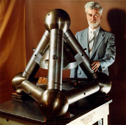
Symmetry is a very important concept when designing a precision measuring instrument. Any asymmetry in a system normally has to be compensated for. In dynamics, it is always better to push or pull a slideway about its axis of reaction otherwise parasitic motions will result due to asymmetry. If a load-bearing structure does not have a suitably designed centre of mass, there will be differential distortion upon loading. It would seem that symmetry should be incorporated into a precision measuring instrument design to the maximum extent. An excellent example of a symmetrical structure (plus many other precision instrument design concepts) is the Tetraform grinding machine developed by Kevin Lindsey at NPL [28,29]. The symmetrical tetrahedral structure of Tetraform can be seen in Figure 3.7. Calculations and experimental results showed that the Tetraform is extremely well compensated for thermal and mechanical fluctuations. Note, that from a practical point of view, the Tetraform design does not scale well, that is it is not suitable for large machines (those with individual members much greater than 1 m).
3.9 Vibration isolation
Most precision measuring instruments require some form of isolation from external and internal mechanical excitations. Where sub-nanometre accuracy is required, it is essential that seismic and sonic vibration is suppressed. This section will discuss some of the issues that need to be considered when trying to isolate a measuring instrument from vibration. The measurement of vibration is discussed in Ref. [30], and vibration spectrum analysis is reviewed in Ref. [31].
3.9.1 Sources of vibration
Different physical influences contribute to different frequency bands in the seismic vibration spectrum, a summary of which is given in Table 3.1 and discussed in Ref. [30].
Table 3.1
Sources of Seismic Vibration and Corresponding Frequencies [30]
| Frequency/mHz | Cause of Vibration |
| <50 | Atmospheric pressure fluctuations |
| 50–500 | Ocean waves (60–90 mHz fundamental ocean wave frequency) |
| >100 | Wind-blown vegetation and human activity |
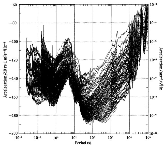
Figure 3.8 shows measured seismic background noise spectra obtained from a worldwide network of 75 seismograph stations. The upper and lower bounds of this data set have been used to model ‘noisy’ and ‘quiet’ vibration environments. The underlying structure of the vibration spectra is determined by the dominant cause of seismic noise at each period band. Short-period (less than 1 s) vibration variations are often dominated by human activity and machinery [32].
For determining the low-frequency vibrations, a gravitational wave detector, in the form of a Michelson interferometer with 20 m arms, has been used to measure vibrations 1 km below sea level [33]. A summary of the results is given in Table 3.2.
Table 3.2
Possible Sources of Very Low-Frequency Vibration
| Source | Period | Acceleration/m·s−1 |
| Earth’s free seismic oscillation | 102–103 s | 10−6–10−8 |
| Core modes | 103 s | 10−11 |
| Core undertone | 103–104 s | 10−11 |
| Earth tides | 104–105 s | 10−6 |
| Post-seismic movements | 1–103 days | 10−6–10−8 |
| Crustal movements | 102 days | 10−7–10−9 |
3.9.2 Passive vibration isolation
Simple springs and pendulums can provide vibration isolation in both vertical and horizontal directions. The transmissibility of an isolator is the proportion of a vibration as a function of frequency that is transmitted from the environment to the structure of the isolator. For a single degree of freedom vibration isolation system, the transmissibility, T, is given by [33]
(3.14)
 (3.14)
where ω0 is the resonant frequency of the isolator and γ is the viscous damping factor. Figure 3.9 shows the transmissibility as a function of frequency ratio for various damping factors.

Vibration isolation is provided only above ![]() times the natural frequency of the system, that is
times the natural frequency of the system, that is
(3.15)
Therefore, to provide vibration isolation at low frequencies, the resonant frequency of the isolation system must be as low as possible. The resonant frequency for a pendulum is given by
(3.16)
and by
(3.17)
for a spring, where g is the acceleration due to gravity, l is the pendulum length, k is the spring constant and m is the mass.
Rewriting Eq. (3.17) in terms of the static extension or compression of a spring, δl, gives
(3.18)
since the static restoring force kδl=mg. Thus, for a low resonant frequency in a spring system, it is necessary to have a large static extension or compression (or use a specialised non-linear spring).
3.9.3 Damping
In vibration isolation systems, it is important to have damping, to attenuate excessive vibration near resonance. In Eq. (3.14), it is assumed that velocity-dependent (viscous) damping is being applied. This is attractive since viscous damping does not degrade the high-frequency performance of the system.
The effects at resonance due to other forms of damping can be represented in terms of an ‘equivalent viscous damping’, using energy dissipation per cycle as the criterion of equivalence [34]. However, in such cases, the value of the equivalent viscous damping is frequency dependent and, therefore, changes the system behaviour. For hysteresis or structural damping, the damping term depends on displacement instead of velocity.
3.9.4 Internal resonances
A limit to high-frequency vibration isolation is caused by internal resonances of the isolation structure or the object being isolated [35]. At low frequencies, the transmissibility is accurately represented by the simple theory given by Eq. (3.14), but once the first resonance is reached, the isolation does not improve. Typically, the fundamental resonance occurs somewhere in the acoustic frequency range. Even with a careful design, it is difficult to make a structure of an appreciable size with internal resonant frequencies above a few kilohertz.
3.9.5 Active vibration isolation
Active vibration isolation is a method for extending the low-frequency isolation capabilities of a system but is very difficult in practice. Single degree of freedom isolation systems are of little practical use because a non-isolated degree of freedom reintroduces the seismic noise even if the other degrees of freedom are isolated. Active vibration isolation uses actuators as part of a control system essentially to cancel out any mechanical inputs. An example of a six degree of freedom isolation system has been demonstrated for an interferometric gravitational wave detector [36].
3.9.6 Acoustic noise
Acoustic noise appears in the form of vibrations in a system generated by ventilators, music, speech, street noise, etc. over a frequency range from about 10 to 1000 Hz in the form of sharp coherent resonances as well as transient excitations [37]. Sound pressure levels in a typical laboratory environment are greater than 35 dB, usually due to air-conditioning systems.
Consider an enclosure that is a simple bottomless rectangular box whose walls are rigidly attached at each edge. When a panel is acoustically excited by a diffuse sound field, forced bending waves govern its sound transmission characteristics, and the sound pressure attenuation is determined by the panel mass per unit area [35]. The panel sound pressure attenuation (dB) is given by [38]
(3.19)
 (3.19)
where ρs is its mass per unit area, ρ0 is the density of air at standard pressure and f is the incident acoustic field frequency. Equation (3.19) suggests that the enclosure wall should be constructed from high-density materials to obtain the largest ρs possible given the load-bearing capacity of any supporting structure. Note that the attenuation decreases for every 20 dB per decade increase in either ρs or frequency.