
Displacement Measurement
Richard Leach
This chapter discusses the various sensing methods used for displacement measurement. Common terms are introduced followed by the two most common forms of displacement interferometry: homodyne and heterodyne. Double pass, differential and swept-frequency absolute distance interferometers are also covered. The various sources of errors associated with displacement interferometry are presented, including thermal, cosine, deadpath and periodic error. Other forms of displacement sensors are then discussed, along with their error sources, including strain sensors, capacitive sensors, eddy current and inductive sensors, optical encoders and optical fibre sensors. Lastly, the calibration of displacement sensors is discussed using both optical and X-ray interferometry.
Keywords
Displacement Measurement; Displacement Interferometer; Homodyne Interferometer; Heterodyne Interferometer; Differential Interferometer; Cosine Error; Deadpath Error; Heydemann Correction; Strain Sensor; Capacitive Sensor; Inductive Sensor; Eddy Current Sensor; Optical Encoder; Optical Fibre Sensor; X-Ray Interferometer
5.1 Introduction to displacement measurement
At the heart of all instruments that measure a change in length, or coordinates, are displacement sensors. Displacement sensors measure the distance between a start position and an end position, for example the vertical distance moved by a surface measurement probe as it responds to surface features. Displacement sensors can be contacting or non-contacting, and often can be configured to measure velocity and acceleration. Displacement sensors can be used to measure a whole range of measurands such as deformation, distortion, thermal expansion, thickness (usually by using two sensors in a differential mode), vibration, spindle motion, fluid level, strain and mechanical shock. Many length sensors are relative in their operation, that is they have no zero or datum. For this type of sensor, the zero of the system is some arbitrary position at power-up. An example of a relative system is a laser interferometer. Many encoder-based systems have a defined datum mark that defines the zero position or have absolute position information encoded on the track. An example of an absolute sensor is a laser time-of-flight system or certain types of angular encoder.
There are many types of displacement sensor that can achieve resolutions of the order of nanometres and less, and only the most common types are discussed here. The reader can consult several modern reviews and books that discuss many more forms of displacement sensor (see, e.g. Refs. [1–4]). Displacement sensors are made up of several components, including the actual sensing device, a transduction mechanism to convert the measurement signal to an electrical signal and signal-processing electronics. Only the measurement mechanisms will be covered here, but there are several comprehensive texts that can be consulted on the transduction and signal-processing systems (see, e.g. Ref. [5]).
5.2 Basic terms
There are number of terms and definitions that are useful when designing or procuring displacement sensors. The following four terms are often used indistinguishably [6].
1. Length – It is the measured dimension of an object. An example is the length of a gauge block, which is measured from one end face to the other (see Chapter 4). In SI units, the unit of length is the metre (see Section 2.3).
2. Distance – It is a quantitative measure of how far two objects are apart. In mathematics, a distance is called a metric. Distance is also measured in metres and is a scalar quantity.
3. Displacement – It is the distance between an initial position and a subsequent position of a moving object, measured in metres. In mathematics, displacement is defined as the shortest path between the final point and the initial point of a body and is a vector quantity.
4. Position – It is the spatial location of an object, quantified as a spatial coordinate and is a vector quantity. Position is always relative to the origin of a one-dimensional coordinate system; a line, such as an axis of a two-dimensional coordinate system; or a plane, such as the reference surface in a three-dimensional coordinate system. In physics, position is the location in space of a physical body. In the rigid-body approximation, where the configuration of that body is fully specified by six generalised coordinates (three linear and three rotational) corresponding to its six degrees of freedom, position is given by the three linear coordinates.
There is also a large range of terms and definitions that are relevant to displacement sensors. The following list is not exhaustive but presents just some of the characteristics that need to be determined when considering a displacement sensor (see Ref. [4] for a thorough review of all these terms):
5.3 Displacement interferometry
5.3.1 Basics of displacement interferometry
Displacement interferometry is usually based on the Michelson configuration or some variant of that basic design. In Chapter 4, we introduced the Michelson and Twyman–Green interferometers for the measurement of static length, and most of the practicalities in using such interferometers apply to displacement measurement. Displacement measurement, being simply a change in length, is usually carried out by counting the number of fringes as the object being measured (or reference surface) is displaced. Just as with gauge block interferometry, the displacement is measured as an integer number of whole fringes and a fringe fraction. Displacement interferometers are typically categorised as either homodyne systems (single frequency) or heterodyne systems (two frequencies). Homodyne displacement interferometers require at least two fringe patterns that are 90° out of phase (referred to as phase quadrature) to allow bidirectional fringe counting and to simplify the fringe analysis. Heterodyne displacement interferometers use a frequency modulation method where the two optical frequencies produce a nominal heterodyne frequency, typically in the megahertz regime. The phase of the measurement signal is then tracked relative to an optical reference that is detected at the heterodyne frequency. Photodetectors and digital electronics are used to count the fringes, and the fraction is determined by electronically sub-dividing the fringe [7]. With this method, fringe subdivisions of λ/1000 are common, giving sub-nanometre resolutions for both heterodyne and homodyne systems. There are many homodyne and heterodyne interferometers commercially available, and the realisation of sub-nanometre accuracies in a practical setup is an active area of research [8,9]. Many of the modern advances in high-accuracy interferometry come from the community searching for the effects of gravitational waves [10].
5.3.2 Homodyne interferometry
Figure 5.1 shows a homodyne interferometer configuration. The homodyne interferometer uses a single frequency, f1, laser beam. Often this frequency is one of the modes of a two-mode stabilised laser (see Section 2.9.3.1). The beam from the stationary reference is returned to the beam splitter with a frequency f1, but the beam from the moving measurement path is returned with a Doppler-shifted frequency of f1±δf. These beams interfere in the beam splitter and enter the photodetector. The Doppler-shifted frequency gives rise to a count rate, dN/dt, which is equal to f (2v/c), where v is the velocity of the retro-reflector and c is the velocity of light. Integration of the count over time, t, leads to a fringe count, N=2d/λ, where d is the displacement being measured.
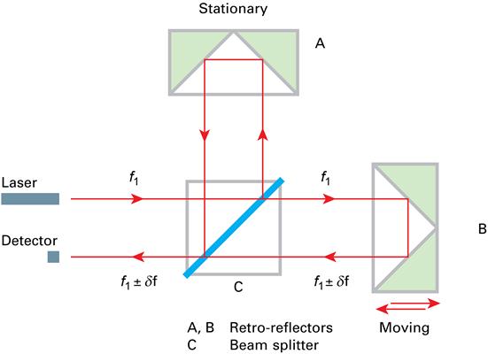
In a typical homodyne interferometer using a polarised beam, the measurement arm contains a quarter-wave plate, which results in the measurement and reference beams having a phase separation of 90° (for bidirectional fringe counting). In some cases, where an un-polarised beam is used [11], a coating is applied to the beam splitter to give the required phase shift [12]. After traversing their respective paths, the two beams re-combine in the beam splitter to produce an interference pattern.
Homodyne interferometers have an advantage over heterodyne interferometers (see Section 5.3.3) because the reference and measurement beams are split at the interferometer and not inside the laser (or at an acousto-optic modulator). This means that the light can be delivered to the interferometer via a standard fibre optic cable. In the heterodyne interferometer, a polarisation-preserving (birefringent) optical fibre has to be employed [13]. Therefore, fibre temperature or stress changes alter the relative path lengths of the interferometer’s reference and measurement beams, causing drift. A solution to this problem is to employ a further photodetector that is positioned after the fibre optic cable [14]; doing so makes it redundant to measure the optical reference prior to the fibre.
Homodyne interferometers can have sub-nanometre resolutions and nanometre-level accuracies, usually limited by their non-linearity (see Section 5.3.8.4). Their speed limit depends on the electronics and the detector photon noise; see also Section 5.3.4. For a speed of 1 m·s−1 and four counts per 0.3 μm cycle, a 3 MHz signal must be measured within 1 Hz. Maximum speeds of 4 m·s−1 with nanometre resolutions are claimed by some instrument manufacturers.
5.3.3 Heterodyne interferometry
Figure 5.2 shows a heterodyne interferometer configuration. The output beam from a dual-frequency laser source contains two orthogonal polarisations, one with a frequency of f1 and the other with a frequency of f2 (separated by about 3 MHz using the Zeeman effect [15] or some other means – see Section 2.9.4). A polarising beam splitter reflects the light with frequency f1 into the reference path. Light with frequency f2 passes through the beam splitter into the measurement path where it strikes the moving retro-reflector causing the frequency of the reflected beam to be Doppler shifted by ±δf. This reflected beam is then combined with the reference light in the beam splitter and returned to a photodetector with a beat frequency of f2−f1±δf. This signal is mixed with the reference signal that continuously monitors the frequency difference, f2−f1. The beat difference, δf, gives rise to a count rate, dN/dt, which is equal to f (2v/c), where v is the velocity of the retro-reflector and c is the velocity of light. Integration of the count over time, t, leads to a fringe count, N=2d/λ, where d is the displacement being measured.
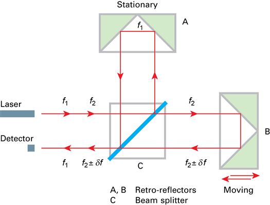
With a typical reference beat of around 3 MHz, it is possible to monitor δf values up to 3 MHz before introducing ambiguities due to the beat crossing through zero. This limits the target speed possible in this case to less than 2 m·s−1 [16], which could be a constraint in some applications. Practical signal processing, and filter roll-off in the electronics, further limits this velocity range. An alternative method of producing a two-frequency laser beam is to use an acousto-optic frequency shifter [17]. This method has the advantage that the frequency difference can be much higher, so that higher count rates can be handled [18].
Many variations on the theme in Figure 5.2 have been developed which improve the speed of response, measurement accuracy and resolution. Modern commercial heterodyne interferometers can be configured to measure both displacement and angle (see, e.g. the xy interferometers in Ref. [19]).
5.3.4 Fringe counting and subdivision
There are two main types of optical fringe counting methods: hardware fringe counting and software fringe counting [20]. Hardware fringe counting utilises hardware circuits to subdivide and count interference fringes [7]. Its principle of operation is as follows. Two interference signals (sine and cosine) with π/2 phase difference are converted into two square waves by means of a zero crossing detector. It is important to employ hysteresis in the zero crossing detectors to ensure spurious noise in the signal does not cause false triggers [21]. Activated by the rising edge of the sine-equivalent square wave, a reversible counter adds or subtracts counts according to the moving direction of the measured object, which is determined by the level of the cosine-equivalent square wave that corresponds to the rising edge of the sine-equivalent square wave. The advantages of the hardware fringe counting method are good real-time performance and relatively simple realisation. However, the electronically countable shift of π/2 corresponds to a phase shift of λ/4 (or λ/8 in a double-pass interferometer – see Section 5.3.5), which defines the resolution limit for most existing hardware fringe counting systems.
Software fringe counting mainly uses digital processing to subdivide and count interference fringes [22]. Its basic principle is that the sine and cosine interference signals, when properly amplified, can be converted by an analogue-to-digital converter (ADC) and then processed by a digital computer to give the number of counts. Compared with hardware fringe counting, software fringe counting can overcome the effect of counting results that are due to random interference signal oscillation and has better intelligence in discriminating the direction of movement. Modern signal processing systems, often called phase meters, typically employ 10–14 bit ADCs with tens of megahertz of measurement bandwidth. The detected signals are then typically processed in a field programmable gate array (FPGA), which can perform massively parallel computations. Commercial phase meters that employ FPGAs typically achieve a further 1:2000 to 1:4000 interpolation factors in addition to the optical resolution. Custom systems have shown even higher interpolations factors (e.g. Refs. [23–25]).
5.3.5 Double-pass interferometry
The simple Michelson interferometer requires a high degree of alignment and requires that alignment to be maintained. Using retro-reflectors relaxes the alignment requirements but it may not always be possible to attach a retro-reflector (usually a cube corner or a cat’s eye) to the target. The Michelson interferometer may be rendered insensitive to mirror tilt misalignment by double-passing each arm of the interferometer and inverting the wavefronts between passes. An arrangement is shown in Figure 5.3, where double passing is achieved with a polarising beam splitter and two quarter-wave plates, and wavefront inversion by a cube-corner retro-reflector. Note that the beams are shown as laterally separated in Figure 5.3. This separation is not necessary but may be advantageous to stop light travelling back to the source. Setting up the components appropriately [26] allows a high degree of alignment insensitivity. Note that such an arrangement has been used in the differential interferometer in Section 5.3.6. The added polarisation components can also increase periodic error that may be present in the measured phase [27,28].

5.3.6 Differential interferometry
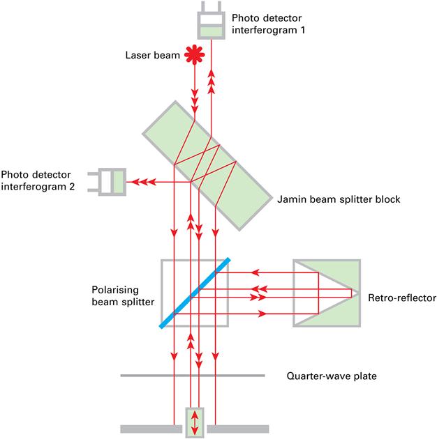
Figure 5.4 is a schema of a differential plane mirror interferometer developed at NPL [29]. The beam from the laser is split by a Jamin beam splitter, creating two beams that are displaced laterally and parallel to each other. Figure 5.4 shows how polarisation optics can be used to convert the Michelson part of the interferometer into a plane mirror configuration, but a retro-reflecting configuration could just as easily be employed. After a double passage through the wave plate, the beams are transmitted back to the Jamin beam splitter where they re-combine and interfere. The design of the Jamin beam splitter coating is such that the two signals captured by the photodetectors are in phase quadrature and so give the optimum signal-to-noise conditions for fringe counting and subdivision. In this configuration only the differential motion of the mirrors is detected.
The differential nature of this interferometer means that many sources of uncertainty are common to both the reference and measurement paths, essentially allowing for common noise rejection. For example, with a conventional Michelson configuration, where the reference and measurement paths are orthogonal, changes in the air refractive index in one path can be different from those in the other path.
Differential interferometers can have sub-nanometre accuracies, as has been confirmed using X-ray interferometry [30]. When a Heydemann correction is applied (see Section 5.3.8.5), such interferometers can have non-linearities of a few tens of picometres.
5.3.7 Swept-frequency absolute distance interferometry
Swept-frequency (or frequency scanning) interferometry using laser diodes or other solid-state lasers is becoming popular due to the versatility of its sources and its ability to measure length absolutely. Currently, such interferometers achieve high resolution but relatively low accuracies and tend to be used for applications over metres. Consider the case of a laser diode aligned to an interferometer of free spectral range, νR. If the output of the laser is scanned through a frequency range νs, N fringes are generated at the output of the interferometer [31]. Provided the frequency scan range is accurately known, the free spectral range and hence the optical path length, L, may be determined from counting the number of fringes. For a Michelson or Fabry–Pérot interferometer in vacuum, the optical path length is given by
(5.1)
It is generally convenient to use feedback control techniques to lock the laser to particular fringes at the start and finish of the scan and so make N integral. For scans of up to several gigahertz, two lasers are typically used, which are initially tuned to the same frequency. One laser is then scanned by νs, and the difference frequency counted directly as a beat by means of a fast detector with several gigahertz of frequency response. This, together with the number of fringes scanned, enables the optical path length to be determined. The number and size of the sweeps can be used to improve the accuracy and range of the interferometer [32].
Swept-frequency interferometers have been used in applications where accurate alignment of components over relatively large distances is required, for example when aligning detectors for particle accelerators [33], for large coordinate measuring machines (CMMs) [34] and for remote sensing applications [35] – in the latter case using frequency combs as the source (see Section 2.6.9).
5.3.8 Sources of error in displacement interferometry
Many of the sources of uncertainty discussed in Section 4.5.4 also apply to displacement interferometry. There will be two types of error sources that will lead to uncertainties. Firstly, there will be error sources that are proportional to the displacement being measured, L, commonly referred to as cumulative errors. Secondly, there will be error sources that are independent of the displacement being measured, commonly referred to as non-cumulative errors. When calculating the measurement uncertainty, the standard uncertainties due to the cumulative and non-cumulative error sources must be combined in an appropriate manner (see Section 2.8.3), and an expanded uncertainty calculated. An example of an uncertainty calculation for the homodyne displacement interferometers on a traceable surface texture measuring instrument is given elsewhere [36], and the most prominent error sources are discussed here.
The effects of the variation in the vacuum wavelength and the refractive index of the air will be the same as described in Section 4.5.4, and the effect of the Abbe error is described in Section 3.4.
5.3.8.1 Thermal expansion of the metrology frame
All measuring instruments have thermal and metrology loops (see Section 3.6). In the case of a Michelson interferometer, with reference to Figure 4.7, both loops run from the laser, follow the optical beam paths through the optics and travel back to the laser via the mechanical base used to mount the optics. Any thermal expansion in these components, for example due to changes in the ambient temperature or conduction into the system from motors, will cause an error in the length measured by the interferometer. Such errors can be corrected for as described in Section 3.7.1 and must be considered in the instrument uncertainty analysis. Thermal expansion errors are cumulative. The change in length due to thermal expansion, Δl, of a part of length, l, is given by
(5.2)
where α is the coefficient of linear thermal expansion and ΔT is the change in temperature.
5.3.8.2 Deadpath length
Deadpath length, d, is defined as the difference in distance in air between the reference and measurement reflectors and the beam splitter when the interferometer measurement is initiated. Deadpath error occurs when there is a non-zero deadpath and environmental conditions change during a measurement. Equation (5.3) yields the displacement, D, for a single-pass interferometer [37]
(5.3)
where N is half the number of fringes counted during the displacement, n2 is the refractive index at the end of the measurement, Δn is the change in refractive index over the measurement time: that is n2=n1+Δn and n1 is the refractive index at the start of the measurement. The second term on the right-hand side of Eq. (5.3) is the deadpath error, which is non-cumulative (although it is dependent on the deadpath length). Deadpath error can be eliminated by presetting counts at the initial position to a value equivalent to d.
5.3.8.3 Cosine error
Figure 5.5 shows the effect of cosine error on an interferometer. The moving stage is at an angle to the laser beam (the scale) and the measurement will have a cosine error, Δl, given by
(5.4)
where l and θ are defined in Figure 5.5. The cosine error will always cause a measurement system to measure short and is a cumulative effect. The obvious way to minimise the effect of cosine error is to correctly align the interferometer. However, despite how perfectly aligned the system appears to be, there will always be a small, residual cosine error. This residual error must be taken into account in the uncertainty analysis of the system. For small angles, Eq. (5.4) can be approximated by
(5.5)

Due to Eq. (5.5), cosine error is often referred to as a second-order effect, contrary to the Abbe error, which is a first-order effect. The second-order nature means that cosine error quickly diminishes as the alignment is improved, but it has the disadvantage that its magnitude is difficult to estimate once it becomes relevant.
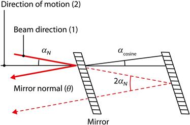
Cosine error for plane mirror targets can also have another uncertainty contributor, even when the input beam propagation direction and the target motion axis are aligned. This occurs when the plane mirror target is not aligned normal to the input beam propagation direction. Thus, the reflected beam from the target propagates off at an angle, causing errors. Equation (5.5) can be expanded to include this error [38],
(5.6)
where θN is the plane mirror misalignment angle between the target surface normal vector at the input beam propagation direction. A schema of this is depicted in Figure 5.6.
5.3.8.4 Periodic error
Both homodyne and heterodyne interferometers are subject to periodic error (sometimes called non-linearities) in the relationship between the measured phase difference and the displacement. Many sources of periodic error in heterodyne interferometers are discussed in Ref. [39], and further discussed, measured and extended in Refs. [40,41]. These sources include misalignment of laser polarisation axes with respect to the beam splitter, ellipticity of the light from the laser source, differential transmission between the two arms of the interferometer, rotation of the plane of polarisation by the retro-reflectors, leakage of light with the unwanted polarisation through the beam splitter and the lack of geometrical perfection of the wave plates used. For homodyne interferometers, the main source of periodic error [42] is attributed to polarisation mixing caused by imperfections in the polarising beam splitters, although there are several other sources [9]. The various sources of periodic error give rise to non-linearities – a first-order phase harmonic having a period of one cycle per fringe and a second harmonic with a period of two cycles per fringe. Errors due to periodic error are usually of the order of a few nanometres but can be reduced to below a nanometre with careful alignment and high-quality optics. There have been many attempts to correct for periodic error in interferometers with varying degrees of success (see, e.g. Refs. [43,44]). Recently, researchers have developed heterodyne interferometers for which a zero periodic error is claimed [45–47].
5.3.8.5 Heydemann correction
When making displacement measurements at the nanometre level, the sine and cosine signals from interferometers must be corrected for dc offsets, differential gains and a quadrature angle that is not exactly 90°. The method described here is that due to Birch [20] and is a modified version of that originally developed by Heydemann [48]. There are many ways to implement such a correction in both software and hardware but the basic mathematics is that presented here. The full derivation is given, as this is an essential correction in many micro- and nanotechnology (MNT) applications of interferometry. This method only requires a single-frequency laser source (homodyne) and does not require polarisation optics. Birch [20] used computer simulations of the correction method to predict a fringe-fractioning accuracy of 0.1 nm. Other methods, which also claim to obtain sub-nanometre uncertainties, use heterodyne techniques [49] and polarisation optics [50].
Heydemann used two equations that describe an ellipse
(5.7)
and
(5.8)
where U1d and U2d represent the noisy signals from the interferometer containing the correction terms p, q and a as defined by Eqs. (5.13), (5.15) and (5.16) respectively, G is the ratio of the gains of the two detector systems and U1 and U2 are given by
(5.9)
(5.10)
where δ is the instantaneous phase of the interferograms. If Eqs. (5.7) and (5.8) are combined, they describe an ellipse given by
(5.11)
If Eq. (5.11) is now expanded out and the terms are collected together, an equation of the following form is obtained
(5.12)
with

Equation (5.12) is in a form suitable for using a linearised least squares fitting routine [51] to derive the values of A through E, from which the correction terms can be derived from the following set of transforms
(5.13)
 (5.13)
(5.14)
(5.15)
(5.16)
(5.17)
Consequently, the interferometer signals are corrected by using the two inversions
(5.18)
and
(5.19)
where ![]() and
and ![]() are now the corrected phase quadrature signals and, therefore, the phase of the interferometer signal is derived from the arctangent of
are now the corrected phase quadrature signals and, therefore, the phase of the interferometer signal is derived from the arctangent of ![]() .
.
The arctangent function varies from −π/2 to +π/2, whereas, for ease of fringe fractioning, a phase, θ, range of 0–2π is preferable. This is satisfied by using the following equation
(5.20)
where θ=0 when U1d>p and Λ=π when U1d<p.
The strong and weak points of a Heydemann-corrected system are that it appears correct in itself and refers to its own result to predict residual deviations (e.g. deviations from the ellipse). However, there are uncertainty sources that still give deviations even when the Heydemann correction is applied perfectly, for example so-called ghost reflections [52] and beam shear [53]. These error sources result in periodic errors at harmonics other than the first or second orders, which is not captured in the underlying model for the Heydemann correction.
5.3.8.6 Random error sources
There are many sources of random error that can affect an interferometer. Anything that can change the optical path or mechanical part of the metrology loop can give rise to errors in the measured displacement. Examples include seismic and acoustic vibration (see Section 3.9), air turbulence (causing random fluctuations of the air refractive index) and electronic noise in the detectors and amplifier electronics. Random errors are usually non-cumulative and can be quantified using repeated measurements.
Homodyne systems measure phase by comparing the intensities of two sinusoidal signals (sine and cosine). By contrast, most modern heterodyne systems measure phase by lock-in detection or single-bin discrete Fourier transforms. Heterodyne systems are less susceptible to beam intensity variations and stray light. However, current signal processing techniques for both systems typically account for these main stray perturbations. Therefore, the influence of noise on both systems is effectively the same.
5.3.8.7 Other sources of error in displacement interferometers
There are many sources of error that only have a significant effect when trying to measure to accuracies of nanometres or less using interferometry. Thermal changes in the metrology loop can also cause direct changes to an interferometer. Most commercial interferometers have a thermal sensitivity specification given in nanometres per kelvin change from nominal ambient conditions. So-called balanced interferometers can have sensitivities of approximately 10 nm K−1, whereas interferometers with unequal paths within the optic can have sensitivities of 300 nm K−1 or greater [54].
Irregularities of the measurement target can also cause significant measurement errors. Lateral motions of the measurement target result in different reflection surface profiles. Deviations in the measurement surface profile directly couple into the measurement value. With cube-corner targets, this error is exacerbated by having three different reflection surfaces and two transition surfaces into the cube corner. With plane mirror targets, improved flatness specifications can reduce this error, but planar positioning systems can exhibit errors similar to crosstalk errors when the target is laterally positioned along an orthogonal axis.
Along with surface irregularities causing error, the uncertainty in the measurement axis location can cause errors in the overall measurement [40,55,56]. For cube-corner targets, the line of measurement is the axis parallel to the incoming optical beam that passes through the nodal point of the cube corner. For plane mirror targets, the line of measurement is the axis parallel to the target normal vector at a location equidistant between the two reflection points on the mirror. This axis should be used for the measurement location for the purposes of calculating the Abbe error described in Section 3.4.
Due to the very high spatial and temporal coherence of the laser source, stray light can interfere with beams reflected from the surfaces present in the reference and measurement arms of the interferometer. The dominant effects are usually due to unwanted reflections and isolated strong point scatterers, both leading to random and non-random spatial variations in the scattered phase and amplitude [17]. These effects can be of the order of a nanometre (see, e.g. Ref. [36]). To minimise the effects of stray reflections, all the optical components should be thoroughly cleaned, the retro-reflectors (or mirrors) should be mounted at a non-orthogonal angle to the beam propagation direction (to avoid reflections off the front surfaces) and all the non-critical optical surfaces should be anti-reflection coated. It is extremely difficult, if not impossible, to measure the amplitude of the stray light, simply because it propagates in the same direction as the main beams. Also, rotational misalignment of polarisation components can increase periodic errors, thus, reducing one error source may give rise to another error source.
Also due to the laser source, the shift of the phase and changes in the curvature of the wavefronts lead to systematic errors and diffraction effects [57]. There will also be quantum effects [58] and even photon bounce [59]. These effects are very difficult to quantify or measure but are usually significantly less than a nanometre.
5.3.9 Latest advances in displacement interferometry
Most of the recent advances in displacement interferometry have been to reduce thermal and mounting errors, make heterodyne interferometry more practical for embedded applications and add inherent multi-axis measurement.
Many commercial interferometers use fused silica optics housed in Invar (a low-expansion steel alloy) mounts that are subsequently bolted together to assemble multi-part interferometers. Mounting the interferometers in this manner increases the overall optical paths within the interferometer, increasing the susceptibility to thermal variations and refractive index fluctuations. For high-accuracy applications, commercial interferometers are now available with all of the optical components mounted to one central optic, typically the beam splitter. Mounting optics in this manner eliminates air gaps in the interferometer assemblies, eliminates some ghost reflections due to reduced glass–air transitions and shortens optical paths, resulting in lower noise interferometers that are more stable over time. The drawback to these single interferometer assemblies is that they are dedicated to a single configuration and cannot be readily disassembled for use in other interferometer configurations.
One advantage that homodyne systems have over heterodyne systems is their ability to readily have the source fibre delivered to the interferometer. Homodyne systems do not use a so-called optical reference to establish the nominal detection frequency. Thus, only one fibre is needed to deliver light to the interferometer, as shown in Figure 5.7. Heterodyne interferometers can be fibre delivered but polarisation-maintaining fibre must be used, an optical reference is needed at each interferometer and periodic errors can still contribute nanometres of error [13]. Spatially separated interferometer configurations [25,46,60–62] offer the possibility of fibre delivery with limited or zero periodic error. In these interferometers, the heterodyne frequency is typically generated using two acousto-optic modulators driven at slightly different radio frequencies (RF). The Wu interferometer configuration has been widely adapted for the LISA programme (see, e.g. Ref. [53]) and can be viewed similarly to a differential interferometer, where the measured signal is the difference between the measurement and reference optical paths. Spatially separated configurations by Tanaka, Joo and Ellis offer the possibility of enhanced optical resolution; however, they cannot be configured as differential interferometers as their measured signal is the total path length changes from both the measurement and reference optical paths.
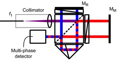
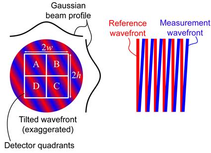
The spatially separated interferometers by Wu et al. [61] and Ellis et al. [25] (shown in Figure 5.8) also use differential wavefront sensing to measure the displacement simultaneously with target tip and tilt. Differential wavefront sensing uses the spatially varying phase from a target’s angle changes incident on a quadrant photodiode to measure four interference patterns [63,64] (Figure 5.9). Then, by knowing the beam size and detector geometry, the measurement target’s angle change can be determined by differencing matched pairs of measured phase from the quadrant photodiode (while the displacement is determined from the average phase over the four quadrants). Differential wavefront sensing has several advantages over traditional single-axis interferometers: (i) the beam size is smaller and only a plane mirror is needed as the target; (ii) the measurement axis location is more readily determined than in traditional plane mirror interferometers; (iii) interferometers for calibration need fewer set-ups to determine linear and angular errors and (iv) the measured phase on the four quadrants has a small spatial location that limits refractive index errors for the angle measurement (the linear measurement is still susceptible to refractive index changes). The downsides to differential wavefront sensing are that it requires extra measurement channels, the wavefront of the interfering beams must be known and aberrations must be limited. Aberrations in the interfering beams can lead to inaccuracies in the sensitivity coefficient, creating uncertainty in the angle measurement [65].

5.3.10 Angular interferometers
In the discussion on angle in Section 2.6, the possibility of determining an angle by the ratio of two lengths was discussed. This method is applicable in interferometry.
Figure 5.10 shows a typical optical arrangement of an interferometer set-up for angular measurements. The angular optics is used to create two parallel beam paths between the angular interferometer and the angular reflector. The distance between the two beam paths is found by measuring the separation of the retro-reflectors in the angular reflector. This measurement is made either directly or by calibrating a scale factor against a known angular standard.

The beam that illuminates the angular optics contains two frequencies, f1 and f2 (heterodyne). A polarising beam splitter in the angular interferometer splits the frequencies, f1 and f2, that travel along separate paths.
At the start position, the angular reflector is assumed to be approximately at a zero position (i.e. the angular measurements are relative). At this position, the two paths have a small difference in length. As the angular reflector is rotated relative to the angular interferometer, the relative lengths of the two paths will change. This rotation will cause a Doppler-shifted frequency change in the beam returned from the angular interferometer to the photodetector. The photodetector measures a fringe difference given by (f1±Df1)−(f2±Df2).
The returned difference is compared with the reference signal, (f1−f2). This difference is related to velocity and then to distance. The distance is then converted to an angle using the known separation of the reflectors in the angular interferometer.
Other arrangements of angular interferometer are possible using plain mirrors, but the basic principle is the same. Angular interferometers are generally used for measuring small angles (less than 10°) and are commonly used for measuring guideway errors in machine tools and measuring instruments.
5.4 Strain sensors
Strain sensors, or strain gauges, are widely used for position control of actuators, especially for piezoelectric actuators (PZTs) [66]. Compared to other displacement sensors, strain gauges are compact, low cost, precise and highly stable.
Due to their low cost and simplicity, resistive strain sensors are one of the most common forms. Resistive strain gauges are constructed from a thin layer of conducting material laminated between two insulating layers. With a zigzag conductive pattern, resistive strain gauges can be designed for high sensitivity in one direction – as the gauge is stretched or compressed in this direction, the resistance changes proportionally. The change in resistance per unit strain is known as the gauge factor. The major disadvantages of resistance strain gauges are the high-measurement noise that arises from the resistive thermal noise and low sensitivity. In addition, the current through the necessary bridge electronics also causes 1/f noise.
Compared to resistive strain gauges, which respond only to changes in geometry, piezoresistive sensors exhibit up to orders of magnitude greater sensitivity. Piezoresistive strain sensors are also easily integrated into standard IC and micro-electromechanical systems (MEMS) fabrication processes. The main disadvantages of piezoresistive sensors are low strain range (0.1 %), high temperature sensitivity, poor long-term stability and non-linearity, although electronic circuits have been designed to partially compensate for these effects. The temperature dependence and low strain range have resulted in piezoresistive sensors primarily being used in micro-fabricated devices (e.g. for atomic force microscope (AFM) [67] and MEMS pressure sensors [68]). Similar to resistive strain gauges, the noise in piezoresistive sensors is predominantly thermal and 1/f noise. However, piezoresistive sensors are essentially semiconductors, the 1/f noise can be worse.
The piezoelectric effect can also be used to produce strain sensors for dynamic applications. The unit cell of a crystalline material with piezoelectric properties will develop a charge dipole when subjected to stress along axes of asymmetry [3]. When inserted into a circuit, applied stress induces transient charge generation which, if collected successfully and integrated, becomes an analogue of strain.
A key advantage of the piezoelectric effect is the ability to generate, as well as measure, strain, as evidenced by the array of advanced nanopositioning devices widely available commercially. This, in principle, enables sensors that can actively interrogate the mechanical properties of passive devices and objects. Macroscopic devices are driven by large applied voltages; in MEMS devices, breakdown limits require exploitation of resonant modes to generate significant strain within allowable voltages.
Combined piezoelectric strain generation and sensing has been successfully applied in a three-dimensional vibrating tactile probe for miniature CMMs ([69], see Chapter 9). In this micro-fabricated probe, which operates near resonance in the kilohertz range, a phase offset between driving and sensing signals is used to detect proximity to a surface to be located in space.
5.5 Capacitive displacement sensors
Capacitive sensors are widely used for non-contact displacement measurement. Capacitive sensors can have very high dynamic responses (up to 100 kHz), sub-nanometre resolution, ranges up to 10 mm, good thermal stability and zero hysteresis (due to their non-contact nature) [70,71]. Capacitive sensors measure the change in capacitance as a target is displaced with respect to the sensor. Figure 5.11 shows a capacitive sensor and measurement target. In this parallel plate capacitor arrangement, the capacitance, C, is given by
(5.21)
where ε is the permittivity of the medium between the sensor and the target, A is the effective surface area of the sensor and d is the distance between the sensor and the target surface. This relationship is not highly dependent on the target conductivity, and hence, capacitance sensors can be used with a range of materials. Note that capacitance sensors can also be used to measure dielectric thickness and density by varying ε and keeping d constant.
Due to the effect of stray capacitance and the need to measure very low values of capacitance (typically from 0.01 to 1 pF), capacitance sensors usually require the use of a guard electrode to minimise stray capacitance. The guard electrode constrains the measurement field to a target spot size of about 130 % of the sensing electrode’s diameter.
Capacitance sensors are used in the semiconductor, disk drive and precision manufacturing industries, often to measure the motion of an axis of rotation, or to control linear position, in high-bandwidth applications, such as fast tool servo control, and high-speed optical focusing. They are also used for level sensing and product sensing, sometimes through a window, sidewall or package. Modern MEMS devices also employ thin membranes and comb-like structures to act as capacitance sensors (and actuators) for pressure, acceleration and angular rate (gyroscopic) measurement [72,73]. High-accuracy capacitance sensors are used for control of MNT motion devices [74] and form the basis for a type of near-field microscope (the scanning capacitance microscope) [75].
The non-linear dependence of capacitance with displacement can be overcome by using a cylindrical capacitor or by moving a flat dielectric plate laterally between the plates of a parallel plate capacitor [76]. These configurations give a linear change of capacitance with displacement. However, most modern commercial sensors use a constant current excitation with the traditional parallel plate capacitive sensor to provide a linear output with displacement.
The environment in which it operates will affect the performance of a capacitance sensor [70]. As well as thermal expansion effects, the permittivity of the dielectric material (including air) will change with temperature and humidity. Misalignment of the sensor and measurement surface will also give rise to a cosine effect.
Capacitance sensors are very similar to some inductive or eddy current sensors (i.e. sensors that use the electromagnetic as opposed to the electrostatic field). Eddy current displacement sensors offer similar measurement capabilities but with very different application-specific considerations. See Ref. [70] for a fuller account of the theory and practice behind capacitive sensors.
5.6 Eddy current and inductive displacement sensors
As discussed above, inductive sensors have similarities to capacitive sensors. However, inductive sensors are not dependent upon the material in the sensor/target gap so they are well adapted to hostile environments where fluids may be present in the gap. They are sensitive to the target material and must be calibrated for each material that they are used with. They also require a certain thickness of target material to operate (usually fractions of a millimetre, dependent on the operating frequency).
A coil in the end of an eddy current sensing probe is excited with an alternating current ranging in frequency from kilohertz to megahertz. The resulting magnetic field surrounds the end of the probe and induces eddy currents in any conductive material near the sensor. The target’s eddy currents produce a magnetic field which opposes the sensor’s field. The magnitude of the eddy currents and the opposing magnetic field are a function of the distance between the probe and the target.
Compared to capacitive sensors, eddy current sensors have larger measurement ranges for the same size probe. Capacitive sensors generally have better signal-to-noise ratios and with their smaller ranges have higher absolute resolutions.
An important consideration in the use of precision eddy current displacement sensors is ‘side loading’. The sensing field of an eddy current sensor is three times larger than the probe diameter. The effective spot size on the target is three times the diameter of the probe, and any other metallic material to the side of the probe that encroaches on the sensing field volume will affect the measurement. More information regarding eddy current sensors and especially their comparison to capacitive sensors is available at www.lionprecision.com/tech-library/technotes/article-0011-cve.html. Whilst they may have nanometre resolutions, their range of operation is usually some millimetres. Their operating frequencies can be 100 kHz and above.
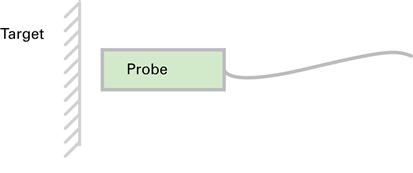
Another popular form of contacting sensor, based on inductive transduction, is the linear variable differential transformer (LVDT). An LVDT probe consists of three coils wound on a tubular former. A centre-tapped primary coil is excited by an oscillating signal of between 50 Hz and 30 kHz and a non-magnetic rod, usually with an iron core, moves in and out of the tube. Figure 5.12 illustrates this design. As the rod moves, the mutual inductance between the primary and two other, secondary, coils changes. A voltage opposition circuit gives an output potential difference that is directly proportional to the difference in mutual inductance of the two secondary coils that is in turn proportional to the displacement of the rod within the tube. When the core is central between the two secondary coils, the LVDT probe is at its null position and the output potential difference is zero.

LVDTs have a wide variety of ranges, typically ±100 μm to ±500 mm and linearities of 0.5 % or better. LVDTs have a number of attractive features. First, there is no physical contact between the movable core and the coil structure, which results in frictionless measurement. The zero output at its null position means that the signal can be amplified by an unlimited amount, and this essentially gives an LVDT probe infinite resolution, the only limitation being caused by the external signal-conditioning electronics. There is complete isolation between the input and the output, which eliminates the need for buffering when interfacing to signal-conditioning electronics. The repeatability of the null position is inherently very stable, making an LVDT probe a good null-position indicator. Insensitivity to radial core motion allows an LVDT probe to be used in applications where the core does not move in an exactly straight line. Lastly, an LVDT probe is extremely rugged and can be used in relatively harsh industrial environments (although they are sensitive to magnetic fields).
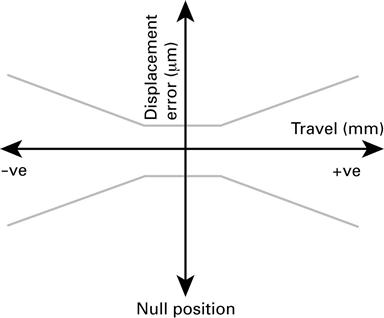
Figure 5.13 shows the ‘bow-tie’ error characteristic of a typical LVDT probe over its linear or measuring range. Probes are usually operated around the null position, for obvious reasons, although, depending on the displacement accuracy required, a much larger region of the probe’s range can be used.
LVDTs find uses in advanced machine tools, robotics, construction, avionics and computerised manufacturing. Air-bearing LVDTs are now available with improved linearities and less damping. Modern LVDTs can have multiple axes [77,78] and use digital signal processing [79] to correct for non-linearities and to compensate for environmental conditions and fluctuations in the control electronics [80].
5.7 Optical encoders
Optical encoders operate by counting scale lines with the use of a light source and a photodetector. They usually transform the light distribution into two sinusoidal electrical signals that are used to determine the relative position between a scanning head and a linear scale. The grating pitch (resolution) of the scales varies from less than 1 μm to several hundred micrometres. As with interferometers, electronic interpolation of the signals can be used to produce sub-nanometre resolution and some of the more advanced optical encoders can have accuracies at this level [81–83].
The most common configuration of an optical encoder is based upon a double grating system; one grating acts as the scale and the other is placed in the reading head. The grating pair produces a fringe pattern at a certain distance from the second grating (usually a Lau or moiré pattern). The reading head has a photodetector that transforms the optical signal into an electrical signal. When a relative displacement between the reading head and the scale is produced, the total light intensity at the photodetector varies periodically. The electronic signals from the photodetector are analysed in the same manner as the quadrature signals from an interferometer (see Section 5.3.4). Figure 5.14 is a schema of a commercial optical encoder system capable of sub-nanometre resolution. The period of the grating is 512 nm. The reading head contains a laser diode, collimating optics and an index grating with a period of 1024 nm (i.e. twice the period of the scale). The signals collected by the detectors are transformed into quadrature signals with a period of 128 nm (i.e. a quarter of the scale period).

There are a number of errors that can affect the performance of an optical encoder, which can be mechanical, electrical or optical [84,85]. Mechanical errors arise from deformation of the parts, thermal expansion and vibration. There may also be errors in the production of the gratings or dust particles on the gratings. Variations in the light intensity, mechanical rotations between the two gratings or variations in the amplification of the optical signals may also occur. Correct design of the scanning head, so that the encoder is robust to variations in the distances between the parts, rotations, variations in illumination conditions, etc., can minimise many of the error sources.
Optical encoders can be encoded with a geometric pattern that describes either the absolute position or the incremental position. Absolute scales contain additional information that can make them physically larger than incremental scales, and hence more sensitive to alignment errors, lower in resolution, slower and more costly.
The highest resolution optical encoders operate on the principle of interference [86]. Light is diffracted through a transparent phase grating in the read head and reflected from a step grating on the scale. Since the technique operates on the principle of diffraction, very small signal periods of down to 128 nm are possible with resolution on the order of a few nanometres [4].
Optical encoders can be linear or rotary in nature. The rotary version simply has the moving grating encoded along a circumference. The linear and angular versions often have integral bearings due to the difficulty of aligning the parts and the necessity for a constant light intensity. Optical encoders are often used for machine tools, CMMs, robotics, assembly devices and precision slideways [87]. A high-accuracy CMM that uses optical encoders is discussed in Section 9.4.1.1. Some optical encoders can operate in more than one axis by using patterned gratings [87,88].
5.8 Optical fibre sensors
Optical fibre displacement sensors are non-contact, relatively cheap and can have sub-nanometre resolution, millimetre ranges at very high operating frequencies (up to 500 kHz). Optical fibres transmit light using the property of total internal reflectance; light that is incident on a media’s interface will be totally reflected if the incident angle is greater than a critical angle (known as Brewster’s angle [89]). This condition is satisfied when the ratio of the refractive index of the fibre and its cladding is in proper proportion (Figure 5.15). The numerical aperture (NA) of an optical fibre is given by
(5.22)
where n1 and n2 are the refractive indexes of the fibre core and cladding, respectively.

This refractive index ratio also governs the efficiency at which light from the source will be captured by the fibre; the more collimated the light from the source, the more light that will be transmitted by the fibre. A multimode optical fibre cable (i.e. one that transmits a number of electromagnetic modes) has a multilayered structure including the fibre, the cladding, a buffer layer, a hard braid and a plastic outer jacket.
There are three types of reflective optical fibre sensors, known as bifurcated sensors: hemispherical, fibre pair and random [90]. These three configurations refer to fibre bundles at one end of the sensor (Figure 5.16).

The bundles have one common end (for sensing) and the other end is split evenly into two (for the source and detector) (Figure 5.17).
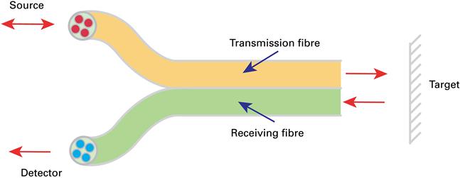
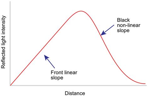
As the target is moved towards the sensing end, the intensity of the reflected light follows the curve as shown in Figure 5.18. Close to the fibre end the response is linear, but follows a 1/d2 curve as the distance from the fibre end increases (d is the distance from the fibre end to the target).
The performance of a bifurcated fibre optic sensor is a function of the cross-sectional geometry of the bundle, the illumination exit angle and the distance to the target surface. Tilt of the target surface with respect to the fibre end significantly degrades the performance of a sensor.
Optical fibre sensors are immune to electromagnetic interference, very tolerant of temperature changes, and bending or vibration of the fibre does not significantly affect their performance. As a consequence, optical fibre sensors are often used in difficult or hazardous environments. Note that only bifurcated fibre optic displacement sensors have been considered here. However, fibre optic sensors can be used to measure a wide range of measurands [91] and can be the basis of very environment-tolerant displacement measuring interferometers [92], often used where there is not sufficient space for bulk optics. Fibre sensing and delivery has been used by some surface topography measuring instruments [93], and fibre sensors are used to measure the displacement of atomic force microscope cantilevers [94].
5.9 Other optical displacement sensors
The sensing element on a point-probing surface topography measuring instrument is essentially a displacement sensor. It is, therefore, possible to use confocal sensors (pinhole- and chromatic-based) and triangulation sensors as displacement sensors. This is especially common for machine tool monitoring (see, e.g. Ref. [95]) and for monitoring rotary motion [87]. The principles and operation of such sensors can be found in Chapter 6.
5.10 Calibration of displacement sensors
There are many more forms of displacement sensors other than those described in this chapter (see Refs. [2–4]). Examples include sensors that use the Hall effect, ultrasonics, magnetism and the simple use of a knife edge in a laser beam [96]. Also, some MNT devices, including MEMS and NEMS sensors, use quantum mechanical effects such as tunnelling and quantum interference [97]. It is often claimed that a sensor has a resolution below a nanometre but it is far from trivial to prove such a statement. Accuracies of nanometres are even more difficult to prove and often there are non-linear effects or sensor/target interactions that make the measurement result very difficult to predict or interpret. For these reasons, traceable calibration of displacement sensors is essential, especially in the MNT regime.
5.10.1 Calibration using optical interferometry
In order to characterise the performance of a displacement sensor, a number of interferometers can be used (provided the laser source has been traceably calibrated; see Section 2.9.5). A homodyne or heterodyne set-up (see Sections 5.3.2 and 5.3.3, respectively) can be used by rigidly attaching or kinematically mounting an appropriate reflector so that it moves collinearly with the displacement sensor. One must be careful to minimise the effects of Abbe offset (see Section 3.4) and cosine error (see Section 5.3.8.3) and to reduce any external disturbances. A differential interferometer (see Section 5.3.6) can also be used but over a reduced range.
As displacement sensor characteristics are very sensitive over short distances, the limits and limiting factors of interferometric systems for very small displacement become critical. For the most common interferometers, it is the periodic error within one wavelength that becomes critical. Even with the Heydemann correction (see Section 5.3.8.5) applied, periodic error can be the major error source.
5.10.1.1 Calibration using a Fabry–Pérot interferometer
The Fabry–Pérot interferometer, as described in Section 4.4.4, can be used for an accurate calibration at discrete positions. If one mirror in the cavity is displaced, parallel interference extrema appear in steps of half a wavelength. If the sensor to be calibrated at the same time measures the mirror displacement, a calibration can be carried out.
Such a system is described elsewhere [98], where it was used to calibrate a displacement generator with a capacitive feedback system with 0.2 nm uncertainty. As a capacitive system can be assumed to have a smoothly varying non-linear behaviour, discrete steps can be feasibly used. However, fringe periodic deviations, as they may appear in interferometric systems, cannot be detected. A continuous calibration system is possible if the wavelength can be tuned and accurately measured simultaneously (see Section 2.9.5).
5.10.1.2 Calibration using a measuring laser
The stability of an iodine-stabilised He–Ne laser is considered to be one part in 1011 (see Section 2.9.3). Relating this stability to the typical length of a laser cavity (a Fabry–Pérot cavity) of, say, 15 cm, one could conclude that the cavity length is fixed with an uncertainty of 1.5 pm. Of course, there are many disturbing factors, such as temperature effects in the air, which make such a small uncertainty in a true displacement measurement difficult to achieve. In the set-up described in Ref. [99], the iodine standard is stabilised on its successive iodine peaks, and a sensor can be calibrated at a number of discrete points. Thermal drift effects mainly determine the uncertainty; the frequency stability itself contributes only 1.5 pm to the uncertainty. This is probably one of the most obvious traceable displacement measurements possible, although difficult to realise in practice.
Separate measuring lasers can be used to give a continuous measurement [100,101]. Here the laser frequency can be tuned by displacing one of its mirrors, while the laser frequency is continuously monitored by a beat measurement. Mounting the laser outside the cavity removes the major thermal (error) source, but further complicates the set-up. In Ref. [102], a piezoelectric controller is used to account for a displacement that is applied to a mirror and is measured by both a sensor and a Fabry–Pérot system. The slave laser is stabilised to the Fabry–Pérot cavity, that is its frequency is tuned such that it gives a maximum when transmitted through the cavity. At the same time, the slave laser frequency is calibrated by a beat measurement against the iodine-stabilised laser. Also here, the uncertainties from the frequency measurement are in the picometre range, and still thermal and drift effects dominate [102].
Design considerations are in the cavity length, the tuning range of the slave laser, the demand that the slave laser has a single-mode operation and the range that the frequency counter can measure. Typical values are 100 mm cavity length and 1 GHz for both the tuning range of the slave laser and the detection range of the photodiode and frequency counter. For a larger frequency range, the cavity length can be reduced, but this increases the demands on the ability to measure a larger frequency range. With tuneable diode lasers, the cavity length can be reduced to the millimetre level, but this requires different wavelength measurement methods [98].
5.10.2 Calibration using X-ray interferometry
The fringe spacing for a single-pass two-beam optical interferometer is equal to half the wavelength of the source radiation and this is its basic resolution before fringe subdivision is necessary. The fringe spacing in an X-ray interferometer is independent of the wavelength of the source; it is determined by the spacing of diffraction planes in the crystal from which X-rays are diffracted [103]. Due to its ready availability and purity, silicon is the most common material used for X-ray interferometers. The atomic lattice parameter of silicon can be accurately measured (by diffraction) and is regarded as a traceable standard of length. Therefore, X-ray interferometry allows a traceable measurement of displacement with a basic resolution of approximately 0.2 nm (0.192 nm for the (220) planes in silicon).
Figure 5.19 shows a schema of a monolithically manufactured X-ray interferometer made from a single crystal of silicon. Three, thin, vertical and equally spaced lamella are machined with a flexure stage around the third lamella (A). The flexure stage has a range of a few micrometres and is driven by a PZT. X-rays are incident at the Bragg angle [12] on lamella B, and two diffracted beams are transmitted. Lamella A is analogous to a beam splitter in an optical interferometer. The transmitted beams are incident on lamella M that is analogous to the mirrors in a Michelson interferometer. Two more pairs of diffracted beams are transmitted and one beam from each pair is incident on lamella A, giving rise to a fringe pattern. This fringe pattern is too small to resolve individual fringes, but when lamella A is translated parallel to B and M, a moiré fringe pattern between the coincident beams and lamella A is produced. Consequently, the intensity of the beams transmitted through lamella A varies sinusoidally as lamella A is translated.

The displacements measured by an X-ray interferometer are free from the periodic error in an optical interferometer (see Section 5.3.8.4). To calibrate an optical interferometer (and, therefore, measure its periodic error), the X-ray interferometer is used to make a known displacement that is compared against the optical interferometer under calibration. By servo-controlling the PZT, it is possible to hold lamella A in a fixed position or move it in discrete steps equal to one fringe period [104]. Examples of the calibration of a differential plane mirror interferometer and an optical encoder can be found in Refs. [30] and [81], respectively. In both cases, periodic errors with amplitudes of less than 0.1 nm were measured once a Heydemann correction (see Section 5.3.8.5) had been applied. More recently, a comparison of the performance of the next generation of optical interferometers was undertaken using X-ray interferometry [8]. X-ray interferometry can also be used to calibrate the characteristics of translation stages in two orthogonal axes [105] and to measure nanoradian angles [106].
One limitation of X-ray interferometry is its short range. To overcome this limitation, NPL, PTB and Instituto di Metrologia ‘G. Colonetti’ (now known as Instituto Nazionale di Recerca Metrologica – the Italian NMI) collaborated on a project to develop the Combined Optical and X-ray Interferometer [107] as a facility for the calibration of displacement sensors and actuators up to 1 mm. The X-ray interferometer has an optical mirror on the side of its moving mirror that is used in the optical interferometer (Figure 5.20). The optical interferometer is a double-path differential system with one path measuring displacement of the moving mirror on the X-ray interferometer with respect to the two fixed mirrors above the translation stage. The other path measures the displacement of the mirror (M) moved by the translation stage with respect to the two fixed mirrors either side of the moving mirror in the X-ray interferometer. Both the optical and X-ray interferometers are servo controlled. The X-ray interferometer moves in discrete X-ray fringes; the servo system for the optical interferometer registers this displacement and compensates by initiating a movement of the translation stage. The displacement sensor being calibrated is referenced to the translation stage and its measured displacement is compared with the known displacements of the optical and X-ray interferometers.
