
Surface Topography Measurement Instrumentation
Richard Leach
This chapter focuses on the measurement of surface topography. The chapter begins with an introduction to the subject and presents a short history. Profile and areal measurements are presented and their pros and cons discussed. Different methods for measuring surface topography are then addressed including stylus methods, triangulation, confocal, chromatic confocal, point autofocus, phase stepping interferometry, coherence scanning interferometry, digital holographic microscopy and scattering instruments. The generic and specific limitations of the optical methods are covered in detail. Calibration and traceability form the last part of the chapter with uncertainty, material measures (calibration artefacts), metrological characteristics, determination of the spatial frequency response and software measurement standards all being discussed.
Keywords
Surface Topography; Profile; Areal; Stylus Instrument; Triangulation; Confocal; Chromatic Confocal; Point Autofocus; Phase Stepping Interferometry; Coherence Scanning Interferometry; Digital Holographic Microscopy; Scattering; Material Measure; Metrological Characteristic; Spatial Frequency Response; Software Measurement Standard; Softgauge
6.1 Introduction to surface topography measurement
Most manufactured parts rely on some form of control of their surface features. The surface is usually the feature on a component or device that interacts with the environment in which the component is housed or the device operates. The surface topography (and of course the material characteristics) of a part can affect things such as how two bearing parts slide together, how light interacts with the part or how the part looks and feels. The need to control and, hence, measure surface features becomes increasingly important as we move into a miniaturised world. The surface features can become the dominant functional features of a part and may become large in comparison to the overall size of an object.
There is a veritable dictionary-sized list of terminology associated with the field of surface measurement. In this book, I have tried to be consistent with ISO specification standards and the NPL good practice guides [1,2]. We define surface topography as the overall surface structure of a part (i.e. all the surface features treated as a continuum of spatial wavelengths), surface form as the underlying shape of a part (e.g. a cylinder liner has cylindrical form) and surface texture as the features that remain once the form has been removed (e.g. machining marks on the cylinder liner) [3]. The manner in which a surface governs the functionality of a part is also affected by the material characteristics and sub-surface physics or surface integrity. Surface integrity is not covered in this book as it falls under material science (see Refs. [4,5]).
In many ways form becomes texture as the overall size of the part approaches that of its surface features, so this distinction is not always clear-cut. In the field of optics manufacturing, the surface form and texture often both need to be controlled to nanometric accuracy. A recent example where the macro-world meets the micro- and nanotechnology (MNT) world is the proposal for a 42 m diameter off-axis ellipsoidal primary mirror for the E-ELT optical telescope [6]. This will be made from several 1.42 m across-flats hexagonal mirror segments that need phenomenal control of their surface topography [7,8]. Such mirrors are not usually thought of as MNT devices, but they clearly need engineering nanometrology. We will only consider surface texture in this book; the measurement of surface form in the optics industry is covered in many other textbooks and references (see, for example, Ref. [9]). Surface texture measurement has been under research for over a century and it was naturally taken up by most of the National Measurement Institutes (NMIs) as their first MNT subject. However, it is still a hot area of research, especially as the new areal surface texture specification standards have now started to be published. The reader is referred elsewhere for more in-depth treatment of the area of surface measurement [10–14].
I have split the information on surface topography measurement in this book into three. Chapters 6 and 7 discuss the instrumentation used to measure surface topography (see Section 6.2 for a discussion of why I have used two instrumentation chapters). Chapter 8 then discusses the characterisation of surface topography – essentially how the data that are collected from a surface topography measuring instrument are analysed.
6.2 Spatial wavelength ranges
A chapter on surface topography, primarily surface texture measurement, could include a large range of instrumentation, with stylus and optical instruments at one end of the range and scanning probe and electron microscopes at the other end. However, this would make for a very large chapter that would include a large range of measurement technologies. I have, therefore, split surface topography into instruments that measure spatial wavelength features that are 500 nm and larger, for example stylus and most far-field optical methods, and instruments that measure features that are 500 nm and smaller, for example scanning probe and electron microscopes. This division is not hard and fast but will suffice to rationalise the information content per chapter.
It is worth noting that the magnitude of 500 nm has not been chosen for purely arbitrary reasons; it is also a form of natural split. The stylus instrument is limited to spatial wavelengths that are greater than the stylus radius, typically 2 μm or more, and far-field optical instruments are diffraction limited, typically to around 300 nm or so. Scanning probe instruments are also limited by the radius of the tip, typically tens of nanometres, and electron microscopes tend to be used for spatial wavelengths that cannot be measured using far-field optical techniques.
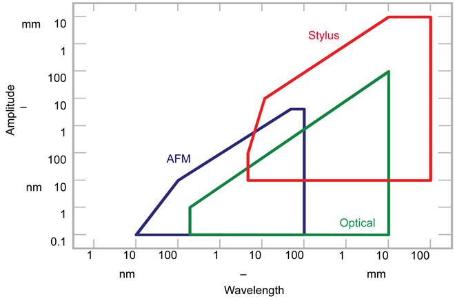
The measurement capabilities of surface texture measuring instruments are constrained by a number of factors, for example range and resolution, tip geometry and environment. Each of these constraints can be modelled and parameterised, and relationships between these parameters derived. The relationships are best represented as inequalities, which define the area of operation of the instrument. A useful way to visualise these inequalities is to construct a space where the constraining parameters form the axes. The constraint relationships (inequalities) can be plotted to construct a polygon. This shape defines the viable operating region of the instrument. Constraints that are linear in a given space must form a flat plane across that space, solutions on one side of which are valid. Such a plane can only form a side of a convex polyhedron containing the viable solutions.
This technique is not new, and the constraint relationships for stylus measuring instruments are well understood. The traditional presentation of a stylus instrument’s operating region in two dimensions is known as amplitude–wavelength (AW) or ‘Stedman’ space, in which constraints are plotted in terms of resolvable surface feature amplitudes and wavelengths [15–17]. The key features of this space are shown in Figure 6.1, with some example plots in Figure 6.2. AW space has been extended recently to include the instrument measuring speed and probing force [18,19].

6.3 Historical background of classical surface texture measuring instrumentation
Before the turn of the nineteenth century, the measurement of surface texture was primarily carried out by making use of our senses of sight and touch. By simply looking at a surface, one can easily tell the difference between a freshly machined surface and one that has been lapped and fine-polished. Touch was utilised by running a finger or fingernail along a surface to be measured and feeling any texture present on the surface. With a few technological modifications, these two methods for measuring surface texture are still the most widely used today.
One of the earliest attempts at controlling surface texture was made in the United States by a company that mounted samples of textures produced by different methods in cases [20] which were given to the machinist, who was expected to obtain a texture on his or her workpiece as near to that specified as possible. This was a suitable method for controlling the appearance of the workpiece but did not in any way indicate the magnitude of the surface texture.
Perhaps the first stylus method was to drag a sapphire needle attached to a pickup arm across the surface being tested [21]. As with a gramophone, the vibration so produced gave rise to sound in a speaker and variation in the electrical current reading on a voltmeter. The method was calibrated by comparing the measured results to those obtained with a sample having a texture that should have been given to the workpiece. This method does not give rise to many benefits over the visual appearance method, and it would be expected that the amplitude of the current reading will bear a greater relation to the pitch of the texture rather than its depth.
Few metrologists can doubt the influence on the world of surface texture measurement, and indeed the entire field of engineering metrology, played by two brothers named Thomas Smithies Taylor and William Taylor, plus their associate William S. Hobson. The three men went into business in Leicester, England, in 1886 manufacturing optical, electrical and scientific instruments [22]. In the 1880s, photography was developing rapidly, and Taylor, Taylor and Hobson (TTH) started making photographic lenses. The present company still holds a leading position in the world for cinematograph and television lenses.
The first metrology instrument manufactured by TTH was a screw diameter measuring machine (originally designed by Eden at NPL). This instrument was used extensively for armaments manufacture during the First World War. In 1945, J. Arthur Rank, the British flour miller and millionaire film magnate, purchased shares in the company. Until 1996, Rank Taylor Hobson was still part of the Rank organisation.
Richard Reason [23], who was employed by TTH, attributed the origin of surface stylus measurements to Gustav Schmaltz of Germany in 1929. Schmaltz used a pivoted stylus drawn over the surface with a very lightweight mirror being attached to the stylus [24]. A beam of light reflected in the mirror traced a graph on a moving photographic chart, providing a magnified, although distorted, outline of the surface profile. In 1934, William Taylor learned of the work of Abbott and Firestone [25] in developing methods for measuring surface texture. In their 1933 paper, Abbott and Firestone discuss the use of a similar instrument to that of Schmaltz and name it a profilograph. Abbott’s instrument was put on the market in 1936. Schmaltz later produced a microscope (known as the light-section microscope) that observed the surface at an angle of incidence of 45°. This gave additional magnification (√2×) to that of the microscope but was only suitable for relatively coarse surface textures since the optical magnification was necessarily limited.
In the mid-1930s, the area where accurate surface measurement was required was mainly in finely finished bearing surfaces, such as those used in aircraft engines. The stylus and mirror arrangement was limited to about 4000× magnification but an order of magnitude more was needed. Therefore, Reason rejected optical magnification and used the principles of a stylus drawn across the surface with a variable inductance pickup and electronic amplification.
Along the lines of Abbott, in 1940 Rolt (at NPL) was pressing for surface texture measurement to produce a single number that would define a surface and enable comparisons to be made. The number most readily obtainable from a profile graph was the Ra parameter (see Section 8.2.7), obtained using a planimeter. Eventually, TTH put the Talysurf onto the market. (Note that the name Talysurf comes from the Latin talea, which roughly translates to ‘measurement’, and not from the name Taylor.) This instrument provided a graph and the average surface roughness value read directly from a metre. Figure 6.3 is a photograph of the original Talysurf instrument.

Another method for measuring surface texture was due to Linnik of the Mendelleif Institute in Leningrad (1930) and interferometers for this method were made by Hilger and Watts and by Pitter Valve Engineering in Britain. These interferometric instruments were diffraction limited but paved the way for a range of non-contacting instruments that is still being increased to date (see Section 6.7).
In 1947, Reason turned his attention to the measurement of roundness, and in 1949, the first roundness testing machine, the Talyrond, was produced. The Talyrond used a stylus arm and electrical transducer operating on the same principle as the Talysurf. These two, plus other instruments, paved the way for the Talystep instrument, which uses the sensitive electronic transducer technique to measure very small steps or discontinuities in a surface and is thus able to measure thin-film steps of near-molecular thickness [26]. Further developments in surface texture measurement will be discussed in the following sections of this chapter.
6.4 Surface profile measurement
Surface profile measurement is the measurement of a line across the surface that can be represented mathematically as a height function with lateral displacement, z(x). With a stylus or optical scanning instrument, profile measurement is carried out by traversing the stylus across a line on the surface. With an areal (see Section 6.7.3) optical instrument, a profile is usually extracted in software after an areal measurement has been taken (see Section 6.5). Figure 6.4 shows the result of a profile measurement extracted from an areal measurement.

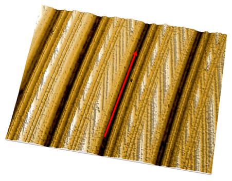
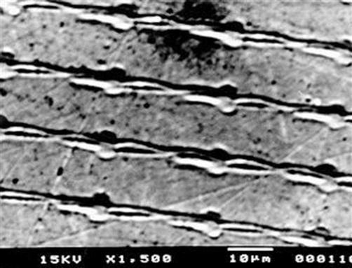
When using a stylus instrument, the traversing direction for assessment purposes is defined in ISO 4287 [27] as perpendicular to the direction of the lay unless otherwise indicated. The lay is the direction of the predominant surface pattern (see Figure 6.5 for an example). Lay usually derives from the actual production process used to manufacture the surface and results in directional striations across the surface. The appearance of the profile being assessed is affected by the direction of the view relative to the direction of the lay, and it is important to take this into account when interpreting surface texture parameters [1,28].
6.5 Areal surface texture measurement
Whereas the profile method may be useful for showing manufacturing process change, much more functional information about the surface can be gained from an analysis of the 3D or ‘areal’ surface topography. Also, over the last few decades, there has been a change in the types of surfaces being used in manufacturing. Previously, stochastic and random surfaces, or the machining marks left by the manufacturing process, were most often used to impart functionality into the surface. More recently, deterministic patterning is being used to critically control the function of a surface [29–33].
To a large extent, the use of deterministic patterning to control function is duplicating the way that surfaces have evolved in the natural world. For example, the riblet micro-structures on a shark’s skin allow it to glide more easily through water [34], and the complex, multi-scale surface structures on the skin of a snake allow it to have unique tribological and thermal properties [35]. Modern manufacturing industry is now using a large range of structuring techniques to affect the function of component parts. Examples include the following (more examples can be found in Ref. [3]):
• surface structuring to encourage the binding of biological implants, for example to promote bone integration and healing [36] or cell adhesion [37];
• micro-optical arrays for displays, lightings, safety signage, backlighters and photo-voltaics [38];
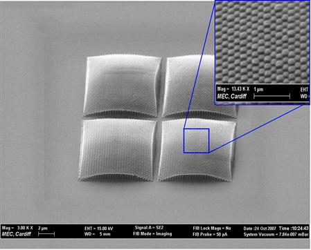
• nanostructured surfaces that affect plasmonic interactions for anti-reflection coatings, waveguides and colour control [39] – recent researchers have attempted to mimic the multi-scale surfaces found in, for example moth-eyes [40,41], see Figure 6.5;
• surfaces of microfluidic channels for flow control, mixing, lab-on-a-chip and biological filtering;
• deterministic patterning to control tribological characteristics such as friction, rheology and wear, for example laser texturing of automotive components [42,43].
There are a number of significant differences between profile and areal analysis. Firstly, most of the structures in the list above require areal characterisation to predict or control their function. Whereas it may be possible to use the profile method to control quality once a machining process has been shown to be sufficiently stable, for problem diagnostics and function prediction, an areal measurement is often required.
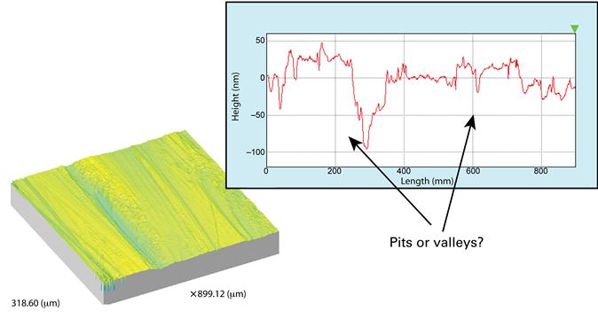
Also, with profile measurement and characterisation, it is often difficult to determine the exact nature of a topographic feature. Figure 6.6 shows a profile and an areal surface map of the same component covering the same measurement area. With the profile alone, a discrete pit is measured on the surface. However, when the areal surface map is examined, it can be seen that the assumed pit is actually a valley and may have far more bearing on the function of the surface than a discrete pit (Figure 6.7).
Lastly, an areal measurement will have more statistical significance than an equivalent profile measurement, simply because there are more data points and an areal map is a closer representation of the ‘real surface’.
To conclude this section, the profile method has been used for over a century, is relatively simple to apply, is well established and is still the most utilised method for surface characterisation in manufacturing industry, especially for process and quality control purposes. But, as manufacturing industry is increasingly using deterministic surface structuring methods to significantly enhance the functionality, efficiency and usefulness of components, areal methods of analysis are becoming more commonplace. However, the complexity of areal analysis, and the fact that an areal measurement can take significantly longer than a profile measurement, means that if profile methods can be used, they should be.
6.6 Surface topography measuring instrumentation
Over the past 100 years, and especially in the last 30 years, there has been a large increase in the number of instruments that are available to measure surface texture. In ISO 25178 part 6 [44], the instruments are divided into three broad classes: line profiling, areal topography measuring and area integrating. Line profiling methods produce a topographic profile, z(x). Areal topography methods produce topographic images, z(x, y). Often, z(x, y) is developed by juxtaposing a set of parallel profiles. Area-integrating methods measure a representative area of a surface and produce numerical results that depend on area-integrating properties of the surface. This chapter will highlight the most popular instruments available at the time of writing – more instruments are discussed elsewhere [10–14]. Scanning probe and electron beam instruments are described in Chapter 7.
6.6.1 Stylus instruments
Stylus instruments are by far the most common instruments for measuring surface texture today, although optical instruments and scanning probe microscopes are becoming more common in manufacturing facilities. A typical stylus instrument consists of a stylus that physically contacts the surface being measured and a transducer to convert its vertical movement into an electrical signal. Other components can be seen in Figure 6.8 and include: a pickup, driven by a motor and gearbox, which draws the stylus over the surface at a constant speed; an electronic amplifier to boost the signal from the stylus transducer to a useful level and a device for recording the amplified signal [1,45,46].

The part of the stylus in contact with the surface is usually a diamond tip with a carefully manufactured shape. Commercial styli usually have tip radii of curvature ranging from 2 to 10 μm, but smaller or larger styli are available for specialist applications and form measurement, respectively. Owing to their finite shape, some styli on some surfaces will not penetrate into valleys and will give a distorted or filtered measure of the surface texture. Consequently, certain parameters will be more affected by the stylus shape than others. The effect of the stylus shape has been extensively covered elsewhere (see, for example Refs. [13,47–50]). The effect of the stylus force can have a significant influence on the measurement results and too high a force can cause damage to the surface being measured (Figure 6.9). ISO 3274 [45] states that the stylus force should be 0.75 mN, but this is rarely checked and can vary significantly from the value given by the instrument manufacturer. The value of 0.75 mN was chosen so as not to cause scratches in metals with a 2 μm radius stylus, but it does cause scratches in aluminium. Smaller forces limit the measurement speed due to the risk of ‘stylus flight’. Some researchers [51–54] have developed constant-force stylus instruments to improve the fidelity between the surface and the stylus tip, plus reduce surface damage and dynamic errors.
To enable a true cross section of the surface to be measured, the stylus, as it is traversed across the surface, must follow an accurate reference path that has the general profile of, and is parallel to, the nominal surface. Such a datum may be developed by a mechanical slideway (e.g. Refs. [55,56]). The need for accurate alignment of the object being measured is eliminated by the surface datum device in which the surface acts as its own datum by supporting a large radius of curvature spherical (or sometimes with different radii of curvature in two orthogonal directions) skid fixed to the end of the hinged pickup. At the front end of the pickup body, the skid rests on the specimen surface (note that skids are rarely seen on modern instruments and not covered by ISO specification standards).
All the aspects of stylus instruments are discussed in great detail elsewhere [13]. The main sources of error associated with a stylus instrument are simply listed below:
• effect of skid or other datum;
• relocation upon repeated measurements;
• effect of filters – electrical or mechanical;
The lateral resolution of a stylus instrument, or the shortest wavelength, λ, of a sinusoidal signal where the probe can reach the bottom of the surface, is given by
(6.1)
where a is the amplitude of the surface and r is the radius of the stylus tip. Note that Eq. (6.1) only applies for a sinusoidal profile (see Ref. [57] for a more thorough treatment of the spatial frequency response of a stylus instrument). Quantisation effects and the noise floor of the instrument will determine the axial, or height, resolution [58].
Modern stylus instruments regularly obtain measurements of surface texture with sub-nanometre height resolution, but traceability of these measurements in each of their axes is relatively new and has not yet been fully taken up in industry [59]. It is worth pointing out here that many of the pitfalls of mechanical stylus techniques are often highly exaggerated [60]. For example, the wear on the surface caused by a stylus is often stated as its fundamental limit, but even if a stylus does cause some damage, this may not affect the functionality of the surface. There have been some proposals to speed up the performance of a stylus by vibrating it axially [61].
A drawback of a stylus instrument when operated in an areal scanning mode is the time to take a measurement. It may be perfectly acceptable to take several minutes to make a profile measurement, but if the same number of points are required in the y-direction (orthogonal to the scan direction) as are measured in the x-direction, then measurement times can be up to several hours. For example, if the drive mechanism can scan at 0.1 mm·s−1 and 1000 points are required for a profile of 1 mm, then the measurement will take 10 s. If a square grid of points is required for an areal measurement, then the measurement time will increase to 105 s or approximately 2.7 h. This sometimes precludes the use of a stylus instrument in a production or an in-line application. A further issue with stylus instruments when used in areal mode is the use of a lateral (y-axis) stage that does not have the same precision and accuracy as the x-axis stage [62]. This is one area where some of the optical instruments offer an advantage over the stylus instruments.
6.7 Optical instruments
There are many different types of optical instrument that can measure surface topography, both surface texture and surface form. The techniques can be broken down into two major areas – those that measure the actual surface topography by either scanning a beam or using the field of view (profile or areal methods) and those that measure a statistical parameter of the surface, usually by analysing the distribution of scattered light (area-integrating methods). Whilst both these methods operate in the optical far field, there is a third category of instruments that operate in the near field – these are discussed in Chapter 7.
The instruments that are discussed in Sections 6.7.2–6.7.4 are the most common instruments that are available commercially. There are many more optical instruments, or variations on the instruments presented here, most of which are listed in ISO 25178 part 6 [44] and discussed in detail in Ref. [14]. At the time of writing, only the methods described in Sections 6.7.2.2, 6.7.3.1, 6.7.3.2 and 6.7.3.4 are being actively standardised in the appropriate ISO committee (ISO 213 working group 16) – see Section 8.2.10 for an overview of the current state-of-play with specification standards in this area.
Optical instruments have a number of advantages over stylus instruments. They do not physically contact the surface being measured and hence do not present a risk of damaging the surface. This non-contact nature can also lead to much faster measurement times for the optical scanning instruments. The area-integrating and scattering methods can be faster still, sometimes only taking some seconds to measure a relatively large area. However, care must be taken when interpreting the data from an optical instrument (compared to that from a stylus instrument). Whereas it is relatively simple to predict the output of a stylus instrument by modelling it as a ball of finite diameter moving across the surface, it is not such a trivial matter to model the interaction of an electromagnetic field with the surface. Often many assumptions are made about the nature of the incident beam or the surface being measured that can be difficult to justify in practice [14,63]. The beam-to-surface interaction is so complex that one cannot decouple the geometry or material characteristics of the surface being measured from the measurement. For this reason, it is often necessary to have an a priori understanding of the nature of the surface before an optical measurement is attempted.
6.7.1 Limitations of optical instruments
Optical instruments have a number of limitations, some of which are generic, and some that are specific to instrument types. This section briefly discusses some of these limitations, and Section 6.13 discusses a number of comparisons that show how the limitations may affect measurements and to what magnitude.
Many optical instruments use a microscope objective to magnify the features on the surface being measured. Most modern optical instruments are designed for infinity-corrected objectives. It is worth noting that the magnification of the objective is not the value assigned to the objective, but the combination of the objective and the microscope’s tube length. The tube length may vary between 160 and 210 mm, and thus, if the nominal magnification of the objective assigned by the manufacturer is based on a 160 mm tube length, then the magnification of this objective on a system with 210 mm tube length will be about 30% greater, as magnification equals tube length divided by the focal length of the objective. Magnifications vary from 2.5× to 200× depending on the application and the type of surface being measured.
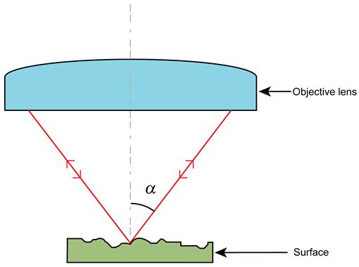
Instruments employing a microscope objective will have two fundamental limitations. Firstly, the numerical (or angular) aperture (NA) determines the largest slope angle on the surface that can be measured and affects the optical resolution. The NA of an objective is given by
(6.2)
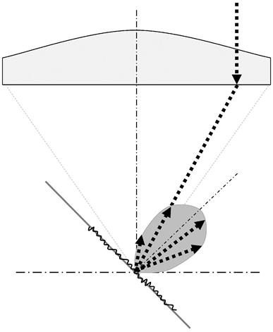
where n is the refractive index of the medium between the objective and the surface (usually air, so n can be approximated by unity) and α is the acceptance angle of the aperture (Figure 6.10, where the objective is approximated by a single lens). The acceptance angle will determine the slopes on the surface that can physically reflect light back into the objective lens and hence be measured. Note that, if there is some degree of diffuse reflectance (scattering) from a rough surface, some light can reflect back into the aperture, allowing larger angles than those dictated by Eq. (6.2) to be detected (Figure 6.11). However, care must be taken when interpreting the data at angles greater than the acceptance angle, and this is still a subject of research [64]. It is also possible to extend the slope limitation with some surfaces using controlled tilting of the sample and specialist image processing [65,66].
For instruments based on interference microscopy, it may be necessary to apply a correction to the interference pattern due to the effect of the NA. Effectively the finite NA means that the fringe distance is not equal to half the wavelength of the source radiation [67–69]. This effect also accounts for the aperture correction in gauge block interferometry (see Section 4.5.4.6), but it has a larger effect here; it may cause a step height to be measured up to 15% short. This correction can usually be determined by measuring a step artefact with a calibrated height value, and it can be directly determined using a grating [70].
The second limitation is the optical resolution of the objective. The resolution determines the minimum distance between two lateral features on a surface that can be measured. The resolution is approximately given by
(6.3)
where λ is the wavelength of the incident radiation [71,72]. For a theoretically perfect optical system with a filled objective pupil, the optical resolution is given by the Rayleigh criterion, where the ½ in Eq. (6.3) is replaced by 0.61 [73]. Yet another measure of the optical resolution is the Sparrow criterion, or the spatial wavelength where the instrument response drops to zero and where the ½ in Eq. (6.3) is replaced by 0.47 [74]. Equation (6.3) and the Rayleigh and Sparrow criteria are often used almost indiscriminately, so the user should always check which expression has been used where optical resolution is a limiting factor. Also, Eq. (6.3) sets a minimum value (although the Sparrow criterion will give a smaller numerical value – this is down to the manner in which ‘resolved’ is defined). If the objective is not optically perfect (i.e. aberration free) or if a part of the beam is blocked (e.g. in a Mirau interference objective or when a steep edge is measured), the value becomes higher (worse). Note also that the above discussion on resolution is only strictly true for incoherent, spatially extended illumination (see Refs. [75,76] for more thorough treatments of the different resolution criteria).
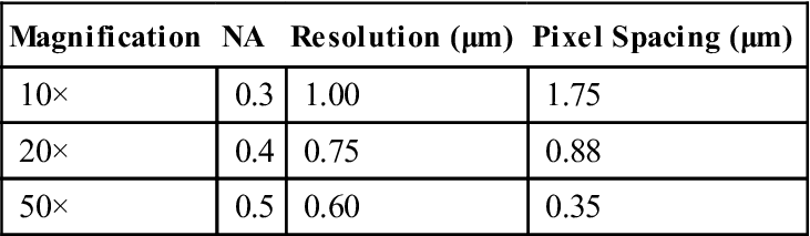
For some instruments, it may be the distance between the pixels (determined by the image size and the number of pixels in the camera array) in the microscope camera array that determines the lateral resolution. Table 6.1 gives an example for a commercial microscope – for the 50× objective, it is the optical resolution that determines the minimum distance between features, but with the 10× objective it is the pixel spacing.
Table 6.1
Minimum Distance Between Features for Different Objectives
| Magnification | NA | Resolution (μm) | Pixel Spacing (μm) |
| 10× | 0.3 | 1.00 | 1.75 |
| 20× | 0.4 | 0.75 | 0.88 |
| 50× | 0.5 | 0.60 | 0.35 |
The optical resolution of the objective is an important characteristic of an optical instrument but its usefulness can be misleading. When measuring surface texture, one must consider the ability to measure the spacing of points in an image along with the ability to accurately determine the heights of features. We need an optical equivalent of Eq. (6.1) for stylus instruments. This is not a simple task, and there may not be a common expression that can be used for all optical instruments. One such definition is the lateral period limit. This is defined as the spatial period of a sinusoidal profile for which the instrument response (measured feature height compared to actual feature height) falls to 50%. The instrument response can be found by direct measurement of the instrument transfer function (see Refs. [77,78]). The lateral period limit and a method to determine its value are discussed in Section 6.12.
Another important factor for optical instruments that magnify the surface being measured is the optical spot size. For scanning-type instruments, the spot size will determine the area of the surface measured as the instrument scans. To a first approximation, the spot size mimics the action of the tip radius on a stylus instrument, that is it acts as a low-pass filter [79] (this is not always the case). The optical spot size is given by
(6.4)
where f is the focal length of the objective lens and w0 is the beam waist (the radius of the 1/e2 irradiance contour at the plane where the wavefront is flat [72]).
In a non-scanning areal instrument, it will be the field of view that determines the lateral area that is measured. In the example given in Table 6.1, the areas measured are 0.3 mm×0.3 mm and 1.2 mm×1.2 mm for the 50× and 10× objectives, respectively.
Many optical instruments, especially those utilising interference, can be affected by the surface having areas that are made from different materials [80,81]. For a dielectric surface, there is a π phase change on reflection (at normal incidence), that is a π phase difference between the incident and reflected beams. The phase change on reflection, δ, is given by
(6.5)
where n and k are the refractive and absorption indexes of the surrounding air (medium 1) and the surface being measured (medium 2), respectively. For dielectrics, k will be equal to zero but for materials with free electrons at their surfaces (i.e. metals and semiconductors), a finite k will lead to a (π−δ) phase change on reflection. For the example of a chrome step on a glass substrate, the difference in phase change on reflection gives rise to an error in the measured height of approximately 20 nm (at a wavelength of approximately 633 nm) when measured using an optical interferometer. A stylus instrument would not be subject to this error in height (although there may be comparable errors due to the different hardness values of the materials). In the example of a simple step, it is common to correct for the phase change on reflection (if one has prior knowledge of the optical constants of the two materials) or an artefact that allows for empirical calibration of the effect. When measuring a multi-material engineered surface or an amalgam, this may not be so easy to achieve and may require in situ characterisation [82].
Most optical instruments can experience problems when measuring features with very high slope angles or discontinuities. Examples include steep-sided vee-grooves, steps or very rough surfaces. The NA of the delivery optics will dictate the slope angle that is detectable and, in the case of a microscope objective, it will be the acceptance angle. For variable focus and confocal instruments (see Sections 6.7.2.2 and 6.7.3.1), sharp, overshooting spikes are seen at the top of steps and often the opposite at the bottom of the step. These are usually caused by the instrument not measuring the topography correctly, sometimes due to only a single pixel spanning the discontinuity. For low-coherence interferometers (see Section 6.7.3.4), there can be problems that are caused by diffraction and interference from the top and bottom surface when a step height is less than the coherence length of the source [83,84]. These effects give rise to patterns known as batwings (Figure 6.12). In general, care should be taken when measuring steep slopes with optical instruments [85].

Many optical instruments for measuring surface topography utilise a source that has an extended spectral bandwidth (e.g. coherence scanning interferometers (CSIs) and confocal chromatic microscopy). Such instruments can be affected by dispersion in the delivery optics or due to thin films at the sample surface. For example, due to dispersion, CSIs can miscalculate the fringe order, giving rise to what are referred to as 2π discontinuities or ghost steps [86]. Dispersion effects can also be field or surface gradient dependent [87]. Also, all optical instruments will be affected by aberrations caused by imperfections in the optical components, and these will affect the measurement accuracy and optical resolution (such systems will not be diffraction limited).
Finally, it is important to note that surface roughness plays a significant role in measurement quality when using optical instrumentation. Many researchers have found that estimates of surface roughness derived from optical measurements differ significantly from other measurement techniques [88–91]. The surface roughness is generally overestimated by optical instrumentation (this is not necessarily true when considering area-integrating instruments), and this may be attributed to multiple scattering. Although it may be argued that the local gradients of rough surfaces exceed the limit dictated by the NA of the objective and, therefore, would be classified as beyond the capability of optical instrumentation, measured values with high signal-to-noise ratio are often returned in practice. If, for example, a silicon vee-groove (with an internal angle of approximately 70°) is measured using coherence scanning interferometry, a clear peak is observed at the bottom of the profile due to multiple reflections (scattering) [92]. Although this example is specific to a highly polished vee-groove fabricated in silicon, this effect may be the cause for overestimation of surface roughness, since a roughened surface can be considered to be made up of lots of randomly oriented grooves with random angles. Note that recent work has shown that, whilst multiple scattering may cause problems in most cases for optical instruments, it is possible to extend the dynamic range of the instrument by using the multiple scatter information. For example, Ref. [93] discusses the measurement of vertical sidewalls and even undercut features using this method.
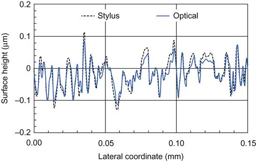
The above limitations notwithstanding, optical instruments for areal topography measurement are highly valued in many industries for their high speed and non-contact nature, for applications ranging from semiconductor wafer metrology to industrial machined-metal quality control. Modern commercial systems can correlate to stylus results within expected uncertainties, as illustrated in Figures 6.13 and 6.14, over a wide range of surface textures [94].

6.7.2 Scanning optical techniques
Scanning optical techniques measure surface topography by physically scanning a light spot across the surface, akin to the operation of a stylus instrument. For this reason, scanning optical instruments suffer from the same measurement-time limitations discussed for stylus instruments (although in many cases the optical instruments can have higher scanning speeds due to their non-contact nature). The measurement will also be affected by the dynamic characteristics of the scanning instrumentation and by the need to combine, or stitch, the optical images together. Stitching can be a significant source of error in optical measurements [95,96], and it is important that the process is well characterised for a given application.
6.7.2.1 Triangulation instruments
Laser triangulation instruments measure the relative distance to an object or a surface. Light from a laser source is projected, usually using fibre optics, on to the surface on which the light scatters. The detector is fitted with optics that focuses the scattered light to a spot on to a CCD-line array or position-sensitive detector. As the topography of the surface changes, this causes the spot to be displaced from one side of the array to the other (Figure 6.15). The line array is electronically scanned by a digital signal-processor device to determine which of the pixels the laser spot illuminates and to determine where the centre of the electromagnetic energy is located on the array. This process results in what is known as sub-pixel resolution, and modern sensors claim to have between five and ten times higher resolution than that of the line array.

Triangulation sensors came to the market at the beginning of the 1980, but initially had many problems. For example, they gave very different measurement results for surfaces with different coefficients of reflectance. So, historically laser triangulation sensors were used in applications where a contact method was not practical or perhaps possible, for example hot, soft or highly polished surfaces. Many of these early problems have now been minimised, and modern triangulation sensors are used to measure a large array of different surfaces, often on a production line.
Triangulation instruments usually use an xy scanning stage with linear motor drives giving a flatness of travel over the typically 150 mm×100 mm range of a few micrometres. Over 25 mm, the flatness specification is usually better than 0.5 μm. These instruments are not designed to have the high resolution and accuracy of the interferometric, confocal or variable focus methods, having typical height resolutions of 100 nm over several millimetres of vertical range. For these reasons, triangulation instruments are used for measuring surfaces with relatively large structure such as paper, fabric, structured plastics and even road surfaces. In Ref. [97], they illustrate the use of high-resolution triangulation for the measurement of fuel cells.
The main benefit of triangulation sensors is the speed with which the measurement can be taken and their robustness for in-process applications. Typical instruments are usually much cheaper than their higher-resolution brethren.
Triangulation instruments do suffer from a number of disadvantages that need to be borne in mind for a given application. Firstly, the laser beam is focused through the measuring range, which means that the diameter of the laser beam varies throughout the vertical range. This can be important when measuring relatively small features as the size of the spot will act as an averaging filter near the beginning and end of the measuring range, as the beam will have a larger diameter here. Also, the measurement depends on an uninterrupted line of sight between laser, surface and detector. Therefore, if a step is to be measured, the sensor must be in the correct orientation so that the laser spot is not essentially hidden by the edge [98]. There can also be effects due to the tilt angle of the surface [99].
Note that triangulation is one form of what is referred to as structured light projection in ISO 25178 part 6 [44]. Structured light projection is a surface topography measurement method whereby a light image with a known structure or pattern is projected on to a surface and the pattern of reflected light, together with knowledge of the incident structured light, allows the surface topography to be determined. When the structured light is a single focused spot or a fine line, the technique is commonly known as triangulation. Structured light methods, for example Moiré fringe projection, are now very common for surface form measurement [100].
6.7.2.2 Confocal instruments
Confocal instruments, the principle of which is shown in Figure 6.16, differ from a conventional microscope in that they have two additional pinhole apertures: one in front of the light source and one in front of the detector [101,102]. The pinholes help to increase the lateral optical resolution over the limits defined by Eq. (6.2) or the Abbe criterion. This resolution enhancement is possible because Abbe assumed an infinitely large field of view. The optical resolution can be increased further by narrowing down the field of view with the pinholes to an area smaller than the Abbe limit [102].
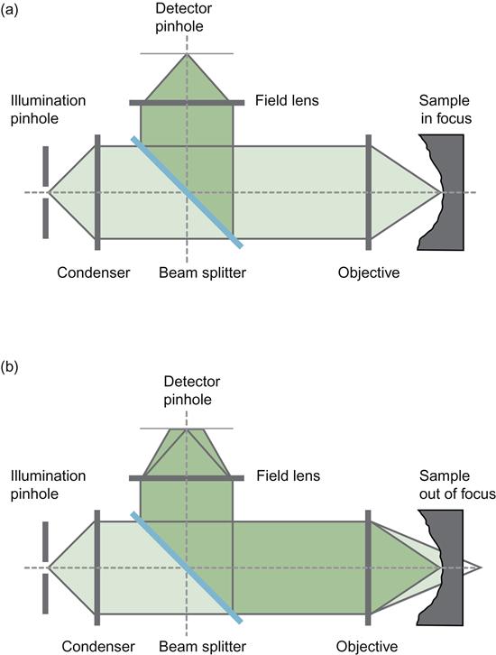
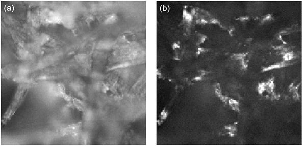
A second effect of the confocal set-up is the depth discrimination. In a normal bright-field microscope set-up, the total energy of the image stays constant while changing the focus. In a confocal system, the total image energy rapidly decreases when the object is moved out of focus [103], as shown in Figure 6.16(b). Only surface points in focus are bright, while out of focus points remain dark. Figure 6.17 shows an example illustrating the difference between normal bright-field imaging and confocal imaging.
When using a confocal instrument to measure a surface profile, a focus scan is needed [102,104]. An intensity profile (confocal curve) whilst scanning through the focus position is shown in Figure 6.18. The location of the maximum intensity is said to be the height of the surface at this point. The full width at half maximum (FWHM) of the confocal curve determines the depth discrimination [105] and is mainly influenced by the objective’s numerical aperture, although it will also be influenced by the type of algorithm applied to calculate the maximum of the confocal intensity profile [102].

Since the confocal principle measures only one point at a time, lateral scanning is needed. The first systems, for example Ref. [106], used a scanning stage moving the sample under the confocal light spot, which is very slow. Modern systems use either scanning mirrors [102] or a Nipkow disk [107] to guide the spot over the measurement area. The Nipkow disk is well known from mechanical television cameras invented in the 1930s. Figure 6.19 shows a classical design of a Nipkow disk. As shown in Figure 6.19, the Nipkow disk is placed at an intermediate image in the optical path of a normal microscope. This avoids the need for two pinholes moving synchronously.

Scanning mirrors are mainly used in confocal laser scanning microscopes, because they can effectively concentrate the whole laser energy on one spot. Their disadvantage is a rather slow scanning speed of typically a few frames per second.
The Nipkow disk is best suited for white light systems, because it can guide multiple light spots simultaneously through the intermediate image of the field of view. It does integrate the whole area within one revolution. Current commercial systems have scanning rates of about 100 frames per second, making a full 3D scan with typically 200–300 frames in a few seconds.
Confocal microscopes suffer from the same limitations as all microscopic instruments as discussed in Section 6.7.1. The typical working distance of a confocal microscope depends on the objective used. Microscope objectives are available with working distances from about 100 μm to a tens of millimetres. With increasing working distance, the NA normally decreases. This results in reduced lateral and axial resolution. Depending on the application, the objective parameters have to be chosen carefully. Low values of NA below 0.4 are in general not suitable for roughness analysis. Low apertures can be used for geometric analysis if the slope angle, ß, is lower than the aperture angle, α, from Eq. (6.1). For an NA of 0.4, ß is approximately 23°.
The vertical measurement range is mainly limited by the working distance of the objective and thus by the NA. Therefore, it is not possible to make high-resolution measurements in deep holes. The field of view is limited by the objective magnification. Lower magnifying objectives with about 10× to 20× magnification provide a larger field of view of approximately one square millimetre. High magnifying objectives with 100× magnification have a field of view of about 150 μm × 150 μm. The lateral resolution is normally proportional to the value given by Eq. (6.2), if it is not limited by the pixel resolution of the camera. However, when the size of the pinhole is small compared to the size of the Airy disk of the incident radiation, there can be an increase in the lateral resolution from that predicted by Eq. (6.2) – what is referred to as the ‘pinhole effect’ [102]. Lateral resolution ranges from 0.25 μm (with a blue source) to about 1.5 μm. The depth resolution can be given by the repeatability of axial measurements and at best has a standard deviation of a few nanometres on smooth surfaces and in suitable environments.
6.7.2.2.1 Confocal chromatic probe instrument
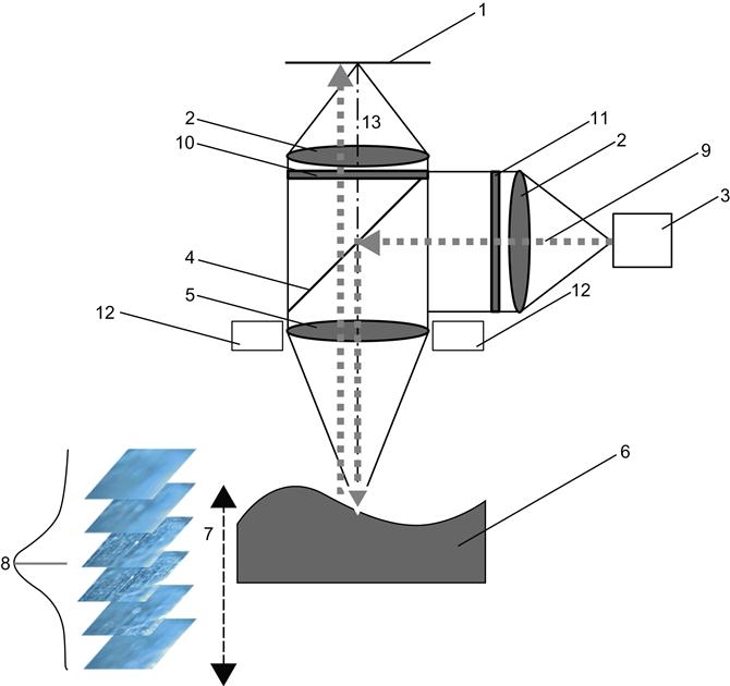
The confocal chromatic probe instrument [108,109] avoids the rather time-consuming depth scan required for an imaging confocal system, by using a non-colour-corrected lens and white light illumination. Due to dispersion along the optical axis, light of different wavelengths is focused at different distances from the objective, as shown in Figure 6.20. By analysing the reflected light with a spectrometer, the confocal curve can be recovered from the spectrum. Closer points are imaged to the blue end of spectrum, while farther points are imaged to the red end [110]. The spectrometer comprises a prism, or an optical grating and a CCD-line sensor to analyse the spectral distribution.

The chromatic principle allows the design of remote sensor heads, coupled only with an optical fibre to the illumination and analysis optics. This is a significant advantage when using chromatic sensors in dirty or dangerous environments. Another advantage of chromatic sensors is the freedom to design the strength of depth discrimination, not only by changing the aperture but also by choosing a lens glass type with appropriate dispersion. Pinhole confocal systems tend to have a smaller working distance with increasing aperture and better depth discrimination. Chromatic systems can be designed to have a large working distance up to a few centimetres while still being able to resolve micrometres in depth.
The principle drawback of chromatic sensors is their limitation to a single measurement point. There has been no success yet in creating a rapidly scanning area sensor. Multi-point sensors with an array of some ten by ten points are available, and there are now systems on the market that can scan a line across the surface [111,112], but these are still some way from a rapid areal scan.
6.7.2.3 Point autofocus profiling
A point autofocus instrument measures surface topography by automatically focusing a laser beam on a point on the specimen surface, moving the specimen surface in a fixed measurement pitch using an xy scanning stage and measuring the specimen surface height at each focused point.
Figure 6.21 illustrates a typical point autofocus instrument operating in beam offset autofocus mode. A laser beam with high focusing properties is generally used as the light source. The input beam passes through one side of the objective, and the reflected beam passes through the opposite side of the objective after focusing on a specimen surface at the centre of the optical axis. This forms an image on the autofocus sensor after passing through an imaging lens.
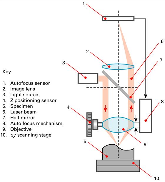
Figure 6.21 shows the in-focus state. The coordinate value of the focus point is determined by the xy scanning stage position and the height is determined from the Z-positioning sensor.
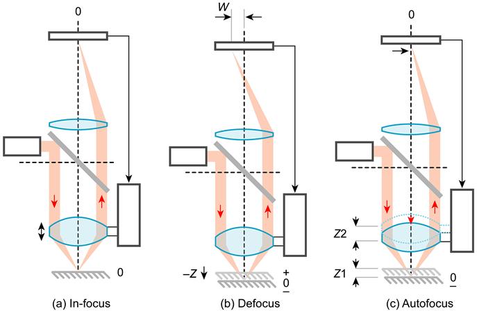
Figure 6.22 shows the principle of point autofocus operation. Figure 6.22(a) shows the in-focus state, where the specimen is in focus, and Figure 6.22(b) shows the defocus state, where the specimen is out of focus. The surface being measured is displaced downward (−Z), and the laser beam position on the autofocus sensor changes accordingly (W). Figure 6.22(c) shows the autofocus state where the autofocus sensor detects the laser spot displacement and feeds back the information to the autofocus mechanism in order to adjust the objective back to the in-focus position. The specimen displacement, Z1, is equal to the moving distance of the objective, Z2, and the vertical position sensor (typically a linear scale is used) obtains the height information of the specimen [113,114].
The disadvantage of the point autofocus is that it requires a longer measuring time than other non-contact measuring methods since it must obtain the coordinate values of each point by moving the mechanism of the instrument (as with chromatic confocal – see Section 6.7.2.2.1). Also, the accuracy of the instrument will be determined by the laser spot size (see Section 6.7.1) because of the uneven optical intensity within the laser spot (speckle) that generates focal shift errors [115].
Point autofocus instruments can have relatively high resolution. The lateral resolution is potentially diffraction limited, but the axial resolution is determined by the resolution of the master scale, which can be down to 1 nm. The range is determined by the xy and z scanner and can be typically 150 mm×150 mm×10 mm. The method is almost immune to the surface reflectance properties since the autofocus sensor detects the position of the laser spot (the limit is typically a reflectivity of 1%). The point autofocus instrument irradiates the laser beam on to a specimen surface that causes the laser beam to scatter in various directions due to the surface roughness of the specimen. This enables the measurement of surface slope angles that are greater than the half aperture angle of the objective (less than 90°) by capturing the scattered light that is sent to the autofocus sensor.
6.7.3 Areal optical techniques
6.7.3.1 Focus variation instruments
Focus variation combines the small depth of focus of an optical system with vertical scanning to provide topographical and colour information from the variation of focus [116,117]. Figure 6.23 shows a schematic diagram of a focus variation instrument. The main component of the system is a precision optical arrangement that contains various lens systems that can be equipped with different objectives, allowing measurements with different lateral resolution. With a beam-splitting mirror, light emerging from a white light source is inserted into the optical path of the system and focused onto the specimen via the objective. Depending on the topography of the specimen, the light is reflected into several directions. If the topography shows diffuse reflective properties, the light is reflected equally strongly into each direction. In the case of specular reflections, the light is scattered mainly into one direction. All rays emerging from the specimen and hitting the objective lens are bundled in the optics and gathered by a light-sensitive sensor behind the beam-splitting mirror. Due to the small depth of field of the optics, only small regions of the object are sharply imaged. To perform a complete detection of the surface with full depth of field, the precision optical arrangement is moved vertically along the optical axis while continuously capturing data from the surface. This ensures that each region of the object is sharply focused. Algorithms convert the acquired sensor data into 3D information and a true colour image with full depth of field. This is achieved by analysing the variation of focus along the vertical axis.
 ); 10, analyser; 11, polariser; 12, ring light; 13, optical axis (
 ).
).Various methods exist to analyse this variation of focus, usually based on the computation of the sharpness at a specific position [117]. Typically, these methods rely on evaluating the sensor data in a small local area. In general, as an object point is focused sharper, the larger the variation of sensor values in a local neighbourhood. As an example, the standard deviation of the sensor values could be used as a simple measure for the sharpness.
The vertical resolution of a focus variation instrument depends on the chosen objective and can be as low as 10 nm. The vertical scan range depends on the working distance of the objective and ranges from a few millimetres to approximately 20 mm or more. The vertical resolution is not dependent upon the scan height, which can lead to a high dynamic range. The xy range is determined by the objective and typically ranges from 0.14 mm×0.1 mm to 5 mm×4 mm for a single measurement. By using special algorithms and a motorised stage, the xy range can be increased to around 100 mm×100 mm.
In contrast to other optical techniques that are limited to co-axial illumination, the maximum measurable slope angle is not dependent on the NA of the objective [64]. Focus variation can be used with a large range of different illumination sources (such as a ring light), which allows the measurement of slope angles exceeding 80°. Additionally, the light can be polarised using appropriate filters (a polariser and an analyser), which allow the removal of specular light components. This is especially helpful for the measurement of metallic surfaces containing steep and flat surface elements. However, as with all instruments that measure angles outside that dictated by the NA, caution must be applied when interpreting the data at such angles.
Focus variation is applicable to surfaces with a large range of different optical reflectance values. Specimens can vary from shiny to diffuse reflecting, from homogeneous to compound materials and from smooth to rough surface properties (but see next paragraph). Focus variation overcomes the aspect of limited measurement capabilities in terms of reflectance by using a combination of a modulated illumination source, controlling the sensor parameters and integrated polarisation. In addition to the scanned height data, focus variation also delivers a colour image with full depth of field that is registered to the 3D data points. Despite the need for vertical scanning, modern focus variation instruments allow the measurement of surfaces within a few seconds, depending on the chosen scanning height and vertical resolution. This is made possible by the use of fast hardware components and sophisticated algorithms for extracting height data from the calculated focus information.
Since focus variation relies on analysing the variation of contrast, it is only applicable to surfaces where the focus varies sufficiently during the vertical scanning process. Surfaces not fulfilling this requirement, such as transparent specimens or components with only a small local roughness, are difficult and sometimes impossible to measure. Typically, focus variation gives repeatable measurement results for surfaces with a local Ra of 10 nm or greater at a λc of 2 μm (see Section 8.2.3).
6.7.3.2 Phase-shifting interferometry
Phase-shifting interferometry (PSI) instrumentation for nanometrology consists of an interference objective integrated with a microscope (Figure 6.24) [85,118,119]. Within the interferometer, a beam splitter directs one beam of light down a reference path, which has a number of optical elements including an ideally flat and smooth mirror from which the light is reflected. The beam splitter directs a second beam of light to the sample where it is reflected. The two beams of light return to the beam splitter and are combined forming an image of the measured surface superimposed by an interference pattern on the image sensor array (camera). The optical path in the reference arm is adjusted to give the maximum interference contrast. During measurement, several known shifts between the optical path to the measured surface and the optical path to the reference mirror are introduced and produce changes in the fringe pattern. A phase map is then constructed from the ensemble of shifted interferograms [120]. There are several ways to shift the difference in optical paths. For example, the objective and reference mirror of the system are translated with the use of a piezoelectric actuator. Finally, the vertical height data are deduced from the phase maps. For specimens with vertical heights greater than half the wavelength, the 2π ambiguity can be suppressed by phase-unwrapping algorithms or the use of dual-wavelength methods [118,121].

PSI microscopes usually come in one of two configurations depending on the arrangement of the microscope objective. Figure 6.25 shows a Mirau configuration, where the components A, B and C are translated with reference to D, and Figure 6.26 shows a Linnik configuration, where components B and C are translated with reference to D and E. The Mirau is more compact and needs less adjustment than the Linnik. For both objectives, there must be white light interference when both the reference mirror and the object are in focus. For the Mirau objective, this is accomplished in one setting of the tilt and position of the reference mirror. For the Linnik objective, both the reference mirror and the object must be in focus, but in addition both arms of the Linnik objective must be made equal within a fringe. Also, a Linnik objective consists of two objectives that must match together [86], at least doubling the manufacturing costs. An advantage of the Linnik is that no central area of the objective is blocked and no space underneath the objective is needed for attaching an extra mirror and beam splitter. Therefore, with the Linnik objective, magnifications and resolutions can be achieved as with the highest-resolution standard optical microscope objectives. A further objective used in PSI is based on a Michelson interferometer (see Section 4.4.1). These are produced by placing a cube beam splitter under the objective lens and directing some of the beam to a reference surface. The advantage of the Michelson configuration is that the central part of the objective is not blocked. However, the cube beam splitter is placed in a convergent part of the beam, which leads to aberrations and limits the instrument to small numerical apertures.


The light source used for PSI measurements typically consists of a narrow band of optical wavelengths as provided by a laser [67], light-emitting diode, narrow-band-filtered white light source or spectral lamp. The accuracy of the central wavelength and the bandwidth of the illumination are important to the overall accuracy of the PSI measurement. The measurement of a surface profile is accomplished by using an image sensor composed of a linear array of detection pixels. Areal measurements of the surface texture may be accomplished by using an image sensor composed of a matrix array of detection pixels. The spacing and width of the image sensor pixels are important characteristics, which determine attributes of instrument lateral resolution (see Section 6.7.1).
PSI instruments can have sub-nanometre axial resolution, but it is difficult to determine their accuracy in a general way, as this can depend on the surface structure being measured. Most of their limitations were discussed in Section 6.7.1. PSI instruments usually require that adjacent points on a surface have a height difference of less than λ/4. The range of PSI is limited to one fringe, or approximately half the central wavelength of the light source, so PSI instruments are most often used for measuring smooth surfaces, such as polished, honed or burnished textures with an Ra or Sa less than λ/10, as opposed to ground, machined or highly structured surfaces. This limitation can be overcome by combining the PSI principles with CSI in one instrument (see Section 6.7.3.4).
The PSI instrument can be used to measure surfaces that are smoother than the reference surface using a process known as reference surface averaging [122]. Alternatively, it may be possible to characterise the reference surface using a liquid surface [123]. Super-polished surfaces are best evaluated using specialised objectives that have no physical reference in focus, obviating the contribution of the internal optics to high-spatial frequency roughness [124].
The xy range in PSI instrumentation will be determined by the field of view of the objective and the camera size. Camera pixel arrays range from 256 × 256 to 1024 × 1024 or more, and the xy range can be extended to several tens of centimetres using scanning stages and stitching software. PSI instruments can be used with samples that have very low optical reflectance values (well below 1%), although the signal-to-noise ratio decreases with an increasing mismatch of the reference and object reflectivities. Optimal contrast is achieved when the reflectance values of the reference and the measured surface match (see Section 4.3.3).
6.7.3.3 Digital holographic microscopy
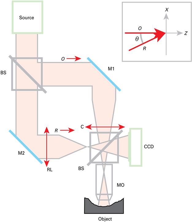
A digital holographic microscope (DHM) is an interferometric microscope very similar to a PSI (see Section 6.7.3.2), but with a small angle between the propagation directions of the measurement and reference beams as shown in Figure 6.27 [125,126]. The acquired digital hologram, therefore, consists of a spatial amplitude modulation with successive constructive and destructive interference fringes. In the frequency domain, the difference between the co-axial geometry (PSI) and the off-axis geometry (DHM) is in the position of the frequency orders of the interference. In PSI, because the three orders (the zeroth-order or non-diffracted wavefront, and ±1 orders or the real and virtual images) are superimposed, several phase shifts are necessary. In contrast, in DHM, the off-axis geometry spatially separates the different frequency orders, which allows simple spatial filtering to reconstruct the phase map from a single digital hologram [127]. DHM is, therefore, a real-time phase imaging technique less sensitive to external vibrations than PSI.
In most DHM instruments, contrary to most PSI instruments, the image of the object formed by the microscope objective is not focused on the camera. Therefore, DHM needs to use a numerical wavefront propagation algorithm that can use numerical optics to increase the depth of field [128] or compensate for optical aberrations [129].
The choice of source for DHM is large but is dictated by the source coherence length. A source with a short coherence length is preferred to minimise parasitic interference, but the coherence length has to be sufficiently large to allow interference over the entire field of view of the detector. Typically, coherence lengths of several micrometres are necessary.
DHM has a similar resolution to PSI [130] and is limited in range to half the central wavelength of the light source when a single wavelength is used. However, dual-wavelength [131] or multiple-wavelength DHM [132] allows the vertical range to be increased to several micrometres. For low magnification, the field of view and the lateral resolution depend on the microscope objective and the camera pixel size; but for high magnification, the resolution is diffraction limited down to approximately 300 nm with a 100× objective. As with PSI, scanning stages and stitching software can be used to increase the field of view.
6.7.3.4 Coherence scanning interferometry
The configuration of a CSI is similar to that of a phase-shifting interferometer, but in CSI a broadband (white light) or extended (many independent point sources) source is utilised [85,133]. CSI is often referred to as vertical scanning white light interferometry or scanning white light interferometry. With reference to Figure 6.28, the light from the broadband light source is directed towards the objective lens. The beam splitter in the objective lens splits the light into two separate beams. One beam is directed towards the sample and one beam is directed towards an internal reference mirror. The two beams recombine and the recombined light is sent to the detector. Due to the low coherence of the source, the optical path length to the sample and the reference must be almost identical, for interference to be observed. Note that coherence is the measure of the average correlation between the values of a wave at any pair of times, separated by a given delay [72]. Temporal coherence tells us how monochromatic a source is. In other words, it characterises how well a wave can interfere with itself at a different time (coherence in relation to CSI is discussed in more detail in Ref. [2] and in general in Section 4.3.4). The detector measures the intensity of the light as the optical path is varied in the vertical direction (z-axis) and finds the interference maximum. Each pixel of the camera measures the intensity of the light and the fringe envelope obtained can be used to calculate the position of the surface.

A low-coherence source is used rather than monochromatic light because it has a shorter coherence length and, therefore, avoids ambiguity in determining the fringe order. Different instruments use different techniques to control the variation of the optical path (by moving either the object being measured, the scanning head or the reference mirror), and some instruments have a displacement-measuring interferometer to measure its displacement [134,135].
As the objective lens is moved, a change of intensity due to interference will be observed for each camera pixel when the distance from the sample to the beam splitter is the same as the distance from the reference mirror to the beam splitter (within the coherence length of the source). If the objective is moved downwards, the highest points on the surface will cause interference first. This information can be used to build up a 3D map of the surface. Figure 6.29 shows how the interference is built up at each pixel in the camera array.

There are a number of options for extracting the surface data from the CSI optical phase data. Different fringe analysis methods give advantages with different surface types, and many instruments offer more than one method. These are simply listed here but more information can be found in Refs. [85,133]. The fringe analysis methods include:
CSI instruments can have sub-nanometre resolution and repeatability, but it is difficult to determine their accuracy, as this will be dependent on the surface being measured. Most of their limitations were discussed in Section 6.7.1 and are reviewed in Ref. [84]. The range of the optical path actuator, usually around 100 μm, will determine their axial range, although this can be increased to several millimetres using a long-range actuator and stitching software. As with PSI, CSI instruments can be used with samples that have low optical reflectance values (well below 1%), although the signal-to-noise ratio decreases with an increasing mismatch of the reference and object reflectivities. Optimal contrast is achieved when the reflectance values of the reference and the measured surface match (see Section 4.3.3).
To avoid the need to scan in the axial direction as in CSI, some areal surface metrology instruments employ multiple or swept wavelength methods. Dispersive white light interferometry generates spectral distributions of the interferograms by means of spectroscopic analysis [136,137] or wavelength scanning [138] without the need for depth scanning. When combined with an additional monitor interferometer to detect vibration, this method promises benefits for in-line applications requiring high immunity to external vibration [139].
CSI techniques can be used to measure relatively large areas (several centimetres) without the need for stitching together of multiple area measurements [140]. Some large-area systems use non-telecentric optics so as to have relatively compact optics [141]. Large-field methods have low magnification and NA, consequently, the lateral resolution is necessarily limited.
Some CSI instruments have been configured to measure the dynamic behaviour of oscillating structures by using a stroboscopic source to essentially freeze the oscillating structure [142,143]. Note that confocal instruments have also been used to measure the motion of vibrating structures [144].
CSI (and PSI) is often used for the measurement of the thickness of optical films by making use of the interference between reflections from the top surface and the different film interfaces [145,146]. Recent advances can also measure the individual thickness of a small number of films in a multilayer stack and the interfacial surface roughness [147].
6.7.4 Scattering instruments
There are various theories to describe the scattering of light from a surface (see Ref. [148] for a thorough introduction and review). The theories are based on both scalar and vector scattering models, and many were developed to describe the scattering of radio waves from the ocean surface. Light scattered from a surface can be both specular, that is the reflection as predicted by geometrical optics, and diffuse, that is reflections where the angle of reflection is not equal to the angle of incidence. Diffuse reflection is caused by surface irregularities, local variations in refractive index and any particulates present at the surface (for this reason, cleanliness is important). From the theoretical models, the amount of light scattered from smooth surfaces is found to be closely related to a statistical parameter of the surface (often Rq or Sq), within a finite bandwidth of spatial wavelengths [149–151]. Hence, scattering instruments do not measure the actual peaks and valleys of the surface texture; rather they measure some aspect of the surface height distribution.
There are various methods for measuring light scatter and there are many commercially available instruments [152,153]. As scattering instruments sample over an area (they are area-integrating methods), they can be very fast and relatively immune to environmental disturbance. For these reasons, scattering methods are used extensively in on-line or in-process situations, for example measuring the effects of tool wear during a cutting process or damage to optics during polishing. It can be difficult to associate an absolute value to a surface parameter measured using a scattering technique, so scattering is often used to investigate process change.
The function that describes the manner in which light is scattered from a surface is the bidirectional scatter distribution function (BSDF) [149]. The reflective properties of a surface are governed by the Fresnel equations [72]. Based upon the angle of incidence and material properties of a surface (optical constants), the Fresnel equations can be used to calculate the intensity of the reflected radiation. The BSDF then describes the intensity of the reflected radiation.
The total integrated scatter (TIS) is equal to the light power scattered into the hemisphere above the surface divided by the power incident on the surface. The TIS is equal to the integral of the BSDF over the scattering hemisphere multiplied by a correction factor (known as the obliquity factor). Davies [154] derived a relationship between the TIS and Rq (or Sq) given by
(6.6)
where the TIS is often approximated by the quotient of the diffusely scattered power to the specularly reflected power.
The instrumentation for measuring TIS [155] consists of a light source (usually a laser), various filters to control the beam size, a device for collecting the scattered light and detectors for measuring the scattered light and specularly reflected light. The scattered light is captured using either an integrating sphere or a mirrored hemisphere (a Coblentz sphere). Often phase-sensitive detection techniques are used to reduce the noise when measuring optical power.
An integrating sphere is a sphere with a hole for the light to enter, another hole opposite where the sample is mounted and a third position inside the sphere where the detector is mounted (Figure 6.30). The interior surface of the sphere is coated with a diffuse white material. Various corrections have to be applied to integrating sphere measurements due to effects such as stray light and the imperfect diffuse coating of the sphere [156].

With a Coblentz sphere, the light enters through a hole in the hemisphere at an angle just off normal incidence, and the specularly reflected light exits through the same hole. The light scattered by the surface is collected by the inside of the hemisphere and focused onto a detector.
A number of assumptions are made when using the TIS method. These include:
• the surface is relatively smooth (λ![]() 4πRq);
4πRq);
• most of the light is scattered around the specular direction;
• scattering originates solely at the top surface and is not attributable to material inhomogeneity or multilayer coatings;
TIS instruments are calibrated by using a diffusing standard usually made from white-diffusing material (material with a Lambertian scattering distribution) [157].
When comparing the Rq value from a TIS instrument to that measured using a stylus instrument, or one of the optical instruments described in Sections 6.7.2 and 6.7.3, it is important to understand the bandwidth limitations of the instruments. The bandwidth limitations of the TIS instrument will be determined by the geometry of the collection and detection optics (and ultimately by the wavelength of the source) [158]. TIS instruments can measure Rq values that range from a few nanometres to a few hundred nanometres (depending on the source). Their lateral resolution is diffraction limited, but often the range of angles subtended by the sphere will determine the lower and upper spatial wavelengths that can be sampled.
Another scattering method that is commercially available is angle-resolved scatter (ARS) [148,151,153,159,160]. However, ARS methods tend to be more complicated than TIS, and the theory relates the ARS to a spectrum of surface spatial wavelengths. Basically, the angular distribution of the scattered light is measured using either a goniophotometer-type instrument or a dedicated scatterometer (see Ref. [153] for examples). The angular distribution of the scattered light can be expressed as the product of an optical factor and a surface factor. The optical factor can be calculated from the illuminating wavelength, the angles of incidence and scattering, the material properties of the surface and the polarisation of the incident and scattered beams. The surface factor is called the power spectral density (PSD) function and is a function of the surface roughness. From the PSD, quantitative values for the height and spatial wavelength distributions can be obtained, although a good a priori model of the surface is required for accurate measurements. It is also possible to extract the BRDF from ARS data. The range and resolution of ARS instruments are very similar to those for TIS instruments. As with TIS instruments, ARS instruments do not measure the actual surface topography but measure some aspect of the height and spatial wavelength distributions. For this reason, ARS instruments are usually employed where process change needs to be monitored.
TIS and ARS instruments are limited in the range of heights that they can measure. With visible illumination, the heights are usually limited to 100 nm or less. The use of infrared illumination sources can increase this range limit. However, to employ scattering to measure larger surface heights, it is more common to use correlation methods, for example the use of laser speckle [161]. Such techniques will not be discussed here, as they are not common to surfaces encountered in MNT applications.
6.8 Capacitive instruments
The use of capacitance to measure surface texture has been around for about as long as stylus methods [162,163]. A conducting plate is held over (or more usually mounted on) a conducting sample to be measured [13]. The capacitance between the plates is a function of the effective plate area, the separation of the plates and the dielectric constant of the medium between them (usually air) [162]. The mean capacitance will change with changes in surface texture as the top plate is scanned over the surface. Surface form can cause serious problems when using capacitance instruments to measure surface texture and, because the capacitance is related to the inverse of the surface texture, large peaks will be weighted differently to valleys.
Note that the configuration described above is usually used to measure proximity (see Section 5.3). Capacitance instruments for measuring surface texture can have significant problems and are difficult to calibrate. They are rarely used nowadays and do not find many applications in the MNT area. However, the scanning capacitance microscope is used in many MNT applications [165].
6.9 Pneumatic instruments
Pneumatic gauging has been around for many years. Basically, an air flow is input to the surface by means of a hollow nozzle and the back pressure generated in the nozzle chamber is measured. This gives rise to a non-linear relationship between surface texture and back pressure, but a linear region exists over a restricted range [166]. The axial resolution can be less than 1 μm and the lateral resolution is limited to the nozzle diameter (usually much greater than 1 μm). Pneumatic gauging can be very fast and is self-purging, which is useful for on-line processes. It is not used extensively for MNT applications.
6.10 Calibration of surface topography measuring instruments
Calibration and traceability for surface texture measuring instruments is a subject area that has received a great deal of attention in the past century and is still an active area of research. There are many unsolved problems and it is still impossible to calibrate a given surface texture measuring instrument for all surface types (this may well always be the case). The complex interaction of the probe with the surface being measured and the vast range of possible surface types confound the problem. This is especially true for optical instruments – it is non-trivial, but possible to calculate the trajectory of a spherical stylus as it traverses a surface, but it is much more difficult to calculate the interaction of an electromagnetic wave with a surface. Also, there is a vast array of surface texture parameters and characterisation methods (see Chapter 8) with varying degrees of complexity. For example, there has been little attempt to calculate the uncertainty associated with areal feature parameters (see Section 8.3.7). The following sections summarise the current state of the art in the area of calibration and traceability.
6.10.1 Traceability of surface topography measurements
Traceability of surface topography measuring instruments can be split into two parts. Firstly, there is the traceability of the instruments and secondly, the traceability of the analysis algorithms and parameter calculations. Instrument traceability is achieved by calibrating the axes of operation of the instrument and its spatial frequency response, usually using calibration artefacts (referred to as material measures in ISO standards and this book). In some instances, it may also be possible to calibrate an instrument using a range of instrumentation to measure the various characteristics of the instrument [167], although this is a time-consuming process that is only usually required by NMIs. Material measures are available in a range of forms for both profile (see Section 6.10.2) and areal calibration (see Section 6.10.3), but a primary instrument must calibrate them (also see penultimate paragraph of this section). Primary instruments are usually kept at the NMIs and can be stylus (e.g. Refs. [53,54,56]) or optical (e.g. Ref. [168]). Most primary instrumentation achieves traceability by using interferometers that are traceable to the definition of the metre via a laser source.
An important aspect of traceability is the measurement uncertainty of the primary instrument, the instrument being calibrated and the parameter calculations. Whilst there is a traceability infrastructure for stylus instruments operating in a profile mode, the infrastructure for areal surface topography measuring instruments is still in its infancy and there are still a number of issues to be addressed. To fill the traceability chain from the definition of the metre to an areal measurement in industry, a number of steps are required (Figure 6.31). Firstly, primary instrumentation that can measure areal surface topography is needed. A number of NMIs (including NPL and PTB) have developed stylus instruments with displacement-measuring laser interferometers that can determine the position of the stylus tip (see, for example Refs. [53,54]). Knowledge of the laser source wavelength in the interferometers assures traceability to the definition of the metre. Secondly, transfer artefacts are needed that can be calibrated via the primary instrumentation (either directly or indirectly) and be used in turn to calibrate instruments in industry. In many cases, it makes commercial sense to calibrate material measures using an optical instrument (such an instrument is much easier to use and faster than the primary instruments) – in this case, the secondary instruments must be calibrated using material measures calibrated on the primary instruments.
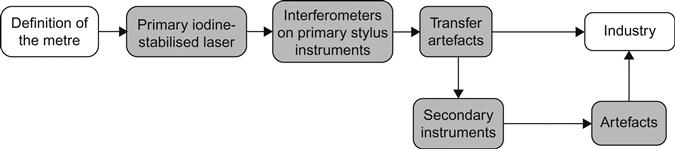
NPL has been working towards a traceability infrastructure for areal measurement for a decade. A stylus-based primary instrument has been developed and methods for calculating uncertainties using this instrument have been devised based on a Monte Carlo approach (see Section 2.8.3.3). NPL (with the University of Huddersfield) recently produced reference software for calculating areal surface texture parameters (at least for the areal field parameters (see Section 6.15) – work on the areal feature parameters is ongoing). NPL (with others in ISO technical committee 213 working group 16) has also developed a series of metrological characteristics which determine the scale calibration of an instrument (see Section 6.12). The remaining task is to determine the spatial frequency response of an instrument. The latter task is still being developed, but see Section 6.14.
For most measurements requiring traceability, a chain of comparisons based on transfer artefacts, usually to an NMI, is appropriate. There is, however, another route to traceability consistent with the requirements of ISO 17025 [169]. In the evaluation of optical surfaces using laser Fizeau interferometry, for example there is no need to employ a transfer artefact to calibrate for the amplification coefficient, as this is based on the He–Ne laser wavelength. Indeed, a procedure based on a mechanical step height would very likely degrade the uncertainty in this case. According to the US standard on metrological traceability [170], ‘Metrological traceability is always to the unit… an appropriate metrological terminus can be… a competent laboratory… or a realisation of the SI metre (sic.)’. This recommendation is reinforced in ISO 17025, which states that ‘Traceability to SI units may be achieved by reference to a natural constant, the value of which … is known and recommended by … the International Committee of Weights and Measures (CIPM)’. CIPM recommendations for standard frequencies and for the practical realisation of the metre appear on the BIPM website (www.bipm.org/en/publications/mep.html), ‘provided that the given specifications and accepted good practice are followed’. A claim of traceability, following this route, for a derived quantity, requires a rigorous uncertainty analysis. This has been documented, in the case of optical flats [171] based on an NIST memorandum [172] ‘… the three flat method is used at NIST to calibrate our master reference flats, the method is very well documented in the technical literature, and provides adequate traceability to satisfy the requirements of ISO 17025’.
A similar approach may be taken with other measurement tasks, including surface texture evaluation using a 3D microscope, provided that we have the appropriate self-calibration means or embedded reference to a natural constant. A specific example is the height response in a CSI instrument, which may be calibrated in situ by integrated metrology using a known wavelength [135,173] or by a capacitance stage sensor or LVDT that has been calibrated using a He–Ne based displacement measuring interferometer.
6.10.2 Material measures for profile measuring instruments
ISO 5436 part 1 [174] describes five types of material measure that are used to calibrate the characteristics of profile measuring stylus instruments. Optical instruments are not covered in ISO 5436 part 1, but many of the material measures described can be adapted to calibrate optical instruments in profile mode. Many groups have developed profile calibration material measures that are available commercially (see Ref. [168] for a review). The use of the five types of profile calibration artefacts is presented in detail in Ref. [1] and they are summarised here ([1] – also presents the analysis methods for the various material measures). Some groups have developed dynamic techniques for calibrating the vertical characteristics of stylus instruments by using a vibrating platform to simulate the spatial frequencies on a surface, but such methods are not used extensively in industry [167,175].
ISO 12179 [176] describes the methodologies to be applied when calibrating a surface texture measuring instrument such as the need for repeat measurements, general instrument set-up and what to include on a calibration certificate. The five types of calibration material measures described in ISO 5436 part 1 [174] are as follows:
1. Type A – used to verify the vertical characteristics of an instrument. They come in two subgroups: type A1 – a wide groove with a flat valley the size of which is dictated by the stylus tip, and type A2 – same as type A1 but with a rounded valley. Figure 6.32 shows how a type A1 material measure is analysed.
2. Type B – used to investigate the geometry of the stylus tip. They come in three subgroups: type B1 – narrow grooves proportioned to be sensitive to the dimensions of the stylus, type B2 – two grids of equal Ra value (see Section 8.2.7.1), one sensitive to the tip dimensions and the other insensitive and type B3 – has a fine protruding edge where the radius and apex angle must be smaller than the radius and apex angle of the stylus being assessed.
3. Type C – used to verify the vertical and horizontal characteristics of an instrument. They consist of a repetitive groove of similar shape with low harmonic amplitudes. They come in four subgroups: type C1 – sine wave profile, type C2 – triangular wave profile, type C3 – sine or triangular wave with truncated peaks and valleys and type C4 – arcuate wave profile.
4. Type D – used to verify the overall performance of an instrument when measuring surface texture parameters. They have an irregular profile in the direction of the traverse (similar to a ground profile) that repeats in the longitudinal direction after some number (usually five) of the sampling lengths (see Section 8.2.3) for which it is designed. The profile shape is constant normal to the measuring direction of the material measure.
5. Type E – used to verify the form measuring capability of the instrument or the straightness of the reference datum slideway (or its equivalent for an optical instrument). They come in two subgroups: type E1 – a spherical dome-shaped material measure that is characterised by its radius and Pt (see Section 8.2.6.5), and type E2 – a precision prism characterised by the angles between the surfaces and Pt on each surface.
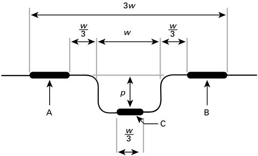
6.10.3 Material measures for areal surface texture measuring instruments
ISO/FDIS 25178 part 70 [177] proposes material measures used as measurement standards to calibrate areal topography measuring instrumentation. The approach chosen in ISO/FDIS 25178 part 70 is to combine the profile material measures described in ISO 5436 part 1 [174] and the newer material measures that can be used to calibrate areal surface topography measuring instruments. Eventually, part 70 will supersede ISO 5436 part 1. A minor inconvenience is that some of the areal and profile material measures are known under different names. In ISO/FDIS 25178 part 70, the material measures are classified as two main types: unidimensional (profile) and bidimensional (areal). Table 6.2 lists the profile material measures, including their new and old terminology, and Table 6.3 lists the areal material measures.
Table 6.2
Types of Unidimensional (Profile) Material Measures
| Areal Type (ISO/FDIS 25178-70) | Current Known Types | Name |
| PPS | 1C1 and B2 | Periodic sinusoidal shape |
| PPR | 1C2 and B2 | Periodic triangular shape |
| PGR | − | Periodic rectangular shape |
| PRO | 1B2 and C4 | Periodic arcuate shape |
| PRI | 1A1 | Groove – rectangular |
| PAS | 1A2 | Groove – circular |
| PDG | 1D1 | Roughness profile |
| PPS | 1D2 | Circular roughness profile |
| PPR | 1E2 | Prism |
| PGR | 1B3 | Razor blade |
| PRO | 1C3 | Approximated sinusoidal shape |
| PRI | CS | Contour standard |
| PAS | ER1 | Double groove |
1ISO 5436-1 types.
Table 6.3
Type of Bidimensional (Areal) Material Measures
| Areal Type (ISO/FDIS 25178: 70) | Current Known Types | Name |
| AGP | ER2 | Grooves – perpendicular |
| AGC | ER3 | Groove – circular |
| ASP | 1E1 | Sphere |
| APS | ES | Plane – sphere |
| ACG | CG1 and CG2 | Cross grating |
| ACS | – | Cross sinusoidal |
| ARS | – | Radial sinusoidal |
| ASG | – | Star-shaped grooves |
| ADT | – | Irregular |
1ISO 5436-1 types.
Type PAS, type AGP and type AGC material measures can be used to calibrate the vertical and horizontal amplification coefficients of the measuring instrument, thus, the instrument x-, y- and z-scale. Type PAS, type AGP and type AGC material measures have a triangular profile groove with a slightly rounded tip. Type PAS material measures have only two parallel grooves (Figure 6.33). Type AGP material measures have four grooves forming a rectangle (Figure 6.34). Type AGC material measures have a circular groove (Figure 6.35). Type AGP and type AGC material measures can also be used to calibrate the squareness of the x- and y-axes.
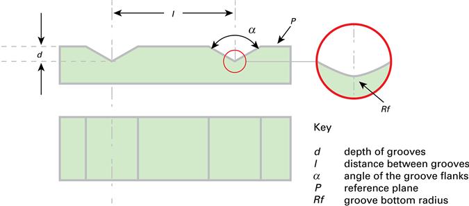

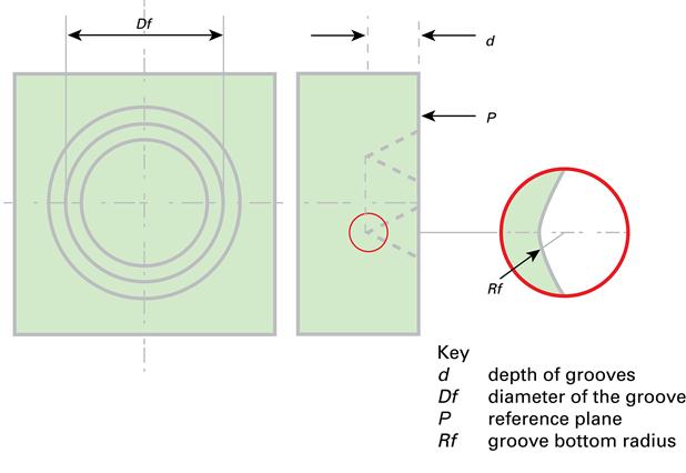
Type APS material measures, referred to as sphere/plane measurement standards, are used to calibrate multiple parameters, such as the vertical and horizontal scales, the squareness of the x- and y-axes, the response curve of the probing system, the stylus geometry (applicable for a pivoting type of stylus) and the stylus tip radius and cone angle. Type APS material measures are composed of a part of a sphere and a plane (Figure 6.36).

Type PRI material measures, referred to as contour standards, are used for overall calibration along one lateral axis of the instrument. Type PRI material measures (Figure 6.37) are composed of at least two arcs of a circle (one concave, one convex) and two wedges/triangles (one concave, one convex).

Type ACG material measures, referred to as cross grating standards, are used to calibrate the amplification coefficients along the instrument axes and the squareness of the x- and y-axes. There are two variants of this type of the material measure: X/Y cross grating material measures have a 2D array of raised lines, grooves or dots and are used to calibrate only the horizontal amplification coefficients and the squareness of the x- and y-axes (Figure 6.38), and X/Y/Z cross grating standards are 2D pits with flat bottoms (waffle patterns, Figure 6.39). X/Y/Z cross grating standards can also be used to calibrate the vertical scale.

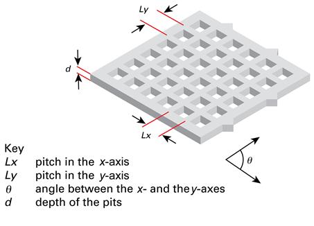
Type ADT material measures (first proposed in Ref. [178]), referred to as irregular topography standards, are used for overall calibration (or more correctly, performance verification) of the measuring instrument. Type ADT irregular topography material measures have a minimum of four unit isotropic measuring areas in a two by two grid (see Figure 6.40 for a three by three grid). The measuring area consists of a limited range of wavelength components. Surface texture parameters, such as Sa, Sq, Sz, Ssk and Sku, are evaluated with uncertainty.

Type ACS material measures are composed of a sinusoidal wavelength along the x-axis and a sinusoidal wavelength along y-axis. Type ACS material measures can be used for overall calibration of the horizontal axis of the instrument and verification of the vertical axis. The measurands are the arithmetic mean height of the surface Sa and root mean height of the surface Sq – the mean pitches along the x- and y-axes can also being used for calibration.
Type ASG, star-shaped groove consists of a series of constant height grooves with triangular profiles in the xy-plane (Figure 6.41). Type ASG material measures are used for verification of the lateral period limit (see Section 6.12).
In some cases, the design of the material measure has to account for particularities of instruments. For example, focus variation instruments are incapable of measuring smooth surfaces (Ra or Sa below 10 nm – see Section 6.7.3.1), and specially designed material measures have to be used.
With the exception of type PDG, type PPS and type ADT, material measures are mainly used for the calibration of the instrument scales. However, not all of the material measures are always required because a large number of the profile material measures are designed for contact stylus instruments, and other material measures can achieve the same measurement goal.
6.11 Uncertainties in surface topography measurement
The calculation of uncertainties for surface topography measurements is a complex task. The greatest complication when calculating uncertainties in surface texture measurement is the contribution of the surface itself. Unlike less complicated measurements, such as displacement, the surface being measured can have a significant effect on the measurement, either by directly affecting the measuring probe or because the surface texture is so variable that repeat measurements in different locations on the surface give rise to a high degree of variability. It is often possible to calculate the instrument uncertainty, that is to say the uncertainty in measuring either (x,z) for profile or (x,y,z) for areal, but when the effect of the surface is taken into account, this uncertainty value may significantly increase, often in an unpredictable manner. Also, the effect of the filtering operation, which essentially ensures that all the measurement points are correlated, is difficult to quantify. Where possible the guidelines in the GUM ([179], see Section 2.8.3) should be applied to calculate instrument uncertainties, and the effect of the surface should be considered in as pragmatic a manner as possible. Examples of methods to calculate the uncertainty in a profile measurement using a stylus instrument are given in Refs. [180,181], but the methods may not be applicable in all circumstances. A rigorous uncertainty is calculated in Ref. [182], using the GUM approach, for the use of a Gaussian profile filter, but little work has been carried out for the uncertainty associated with areal parameters [183].
When the uncertainty due to the instrument has been calculated, it is then often necessary to find the uncertainty in due to a parameter calculation. Once again, this is far from trivial and often the guidelines in the GUM cannot be easily applied. The problem is that for roughness parameters, some characteristics of a roughness measuring instrument have an obvious influence on a roughness parameter, but for others this influence is highly unclear. For example, for an Ra value, it is obvious that an uncertainty of 1% in the vertical axis calibration results in a 1% uncertainty in the Ra value, but it is far less clear what will be the effect if the probe diameter is 5 or 10 µm, instead of the standard 2 µm, or what happens if the cut-off filter is not exactly Gaussian. For a spatial parameter such as RSm, the uncertainty in the vertical direction will not be significant, but the x-ordinate calibration is essential. Moreover, such effects are surface dependent; a very fine surface will be more sensitive for probe diameter deviations and deviations in the short-wavelength cut-off filter than a surface where most of the undulations are far within the wavelength band [184].
Traceability for parameter calculations can be carried out by using calibrated artefacts that have associated known parameters values, for example the type D artefacts (see Section 6.10.2) used for calibrating profile measuring instruments. However, the parameter calculations themselves should be verified using software measurement standards (see Section 6.15), and for the calibrated artefact, an uncertainty has to be stated by those institutions that can calibrate these standards.
There have been a number of experimental [167] and simulation [185,186] studies that have investigated the various influence factors when calculating profile parameters. However, for areal surface topography measurements, there has only been limited research into measurement uncertainty. A rigorous uncertainty analysis has been carried out for the NPL primary areal surface topography measuring instrument [187], and guidelines for estimating the uncertainty contributions due to the ISO metrological characteristics are presented in the NPL good practice guides on areal topography measuring instrument calibration [188–191]. However, there is still a need for methods to estimate uncertainties when using the transfer function approach (see Section 6.14).
6.12 Metrological characteristics
The calibration process for a surface topography measuring instrument should involve the determination of the characteristics of the scales of the instrument and a determination of the instrument’s spatial frequency response. Often the latter part of this process is overlooked and an instrument is considered ‘calibrated’ if only the characteristics of the scales have been determined. With this limited calibration, it is then perfectly feasible to use the instrument to measure linear characteristics, for example step height or lateral spacing, but not for the measurement of a complex surface, where the ability to measure slopes and curvature needs to be determined. This section will consider the instrument scales (and associated resolution), and Section 6.14 will consider the calibration of the spatial frequency response.
NPL has developed methods to determine the metrological characteristics defined by ISO using a set of low-cost material measures (Figure 6.42). These methods and artefacts can be used with NPL measurement good practice guides, which have been published for stylus instruments [188], coherence scanning interferometry [189], imaging confocal microscopy [190] and focus variation microscopy [191]. These guides can also be used with other types of areal surface topography measuring instruments with a little adjustment.

An areal surface topography measuring instrument provides a 3D map of a surface. The 3D map is made up of a set of points measured with respect to three orthogonal length scales. The scales of an areal surface topography measuring instrument are nominally aligned to the axes of a Cartesian coordinate system. The axes are physically realised by various components that are part of the metrological loop of the instrument. Hence, the quality and the mutual position of these components partially confer the quality of the coordinate measurements. The coordinate measurements produced by areal surface topography measuring instruments are also affected by other influence factors, such as ambient temperature, mechanical noise and electrical noise. The effect of a single influence factor, or a combination of influence factors, on the quality of the areal measurements is quantified by experimentally determining the metrological characteristics of the instrument. Typically, these characteristics include the noise of the instrument; the linearity, amplification and resolution of the scales; the deviation from flatness of the areal reference and the squareness of the axes [58,62,192]. The magnitude of the influence factors on an areal measurement can be different for different sizes of measuring area and sampling distance, that is to say the measurement bandwidth. The choice of measurement bandwidth is application dependent and is based on the selection of S-filters and L-filters/F-operators (see Section 8.3.2), each having a range of preset values termed nesting indexes [3,193]. The calibration of an instrument is usually performed using the same conditions as those used on a daily basis.
The calibration of the scales involves a series of relatively simple tasks that are performed to evaluate the magnitude of the uncertainty associated with the metrological characteristics of the instruments, assuming well-defined measuring conditions. The calibration process also necessitates the use of the previously defined material measures designed for calibrating surface topography measuring instruments. The metrological characteristics, defined in draft ISO standards (ISO/CD 25178-600 [194]), that influence the uncertainty associated with the coordinate measurements produced by areal surface topography measuring instruments are measurement noise, deviation of flatness of the areal reference, the amplification coefficient and the linearity of the scales (axial and lateral scales), the squareness of the axes and resolution.
6.13 Comparisons of surface topography measuring instruments
Many comparisons of surface topography measuring instruments have been conducted over the years. The spreads in the results can be quite alarming, especially when comparing contact and non-contact instruments. The authors of such comparisons are often surprised by the results but, upon closer inspection, most of the results can be explained. Often it is stated that the instruments do not compare because they have not been adequately calibrated. Whilst this may be a source of discrepancy, there are usually better reasons for instruments with different operating principles not comparing well. For example, a stylus acts as if a ball is rolled across the surface whilst an optical instrument relies on the reflection of an electromagnetic wave. Is it really so difficult to appreciate that such instruments can produce different results? Also, different instruments will sample different spatial wavelength bandwidths of the surface being measured and will have different physical limitations. Leach and Haitjema [57] give advice on how to achieve compatible results with surface texture comparisons.
In an early example [195], the measurement of groove depths was compared, where this groove could be measured by optical, mechanical and even atomic force microscope (AFM) instruments (see Chapter 7). From this comparison, it became evident that grooves of some 40 nm could be measured with uncertainties in the nanometre level, but, for a 3 μm depth the results scattered far more than 1%, even between NMIs. It is expected that since then, this situation has improved (see last paragraph of this section).
For example, the results of the measurements of a nickel sinusoid sample, with a period of 8 μm and an Ra of 152 nm, showed very different results for a number of different instruments (Figure 6.43) [196]. The participants in this comparison were all experienced in surface texture measurement. In this example, NS IV refers to the traceable instrument at NPL (see Section 6.10.1), Stylus 1 and Stylus 2 are different stylus instruments on the same site, Inter 1 and Inter 2 are the same model of CSI instrument on different sites and Conf refers to a confocal instrument. It was later found out that Stylus 2 had incorrectly applied a filter. A further triangulation instrument was also used in the comparison and the result was an Ra value of 2955 nm – far too large to plot on this figure.

Many of the discrepancies above were explained after the comparison, but the question remains: Would a user in an industrial situation have the luxury of the hindsight that is afforded in such a comparison?
This section is not intended to scare the reader into complete distrust of surface topography instruments – its purpose is to make the reader vigilant when measuring and characterising surface topography. Instruments should be properly calibrated, results should be scrutinised and, where possible, different instruments should be used to measure the same surface. Once a stable measurement procedure is set up in a given situation, appropriate procedures should be in place to ensure that the instrument is operated within its limits and results are properly interpreted. Due care should especially be given to the types of filtering that are applied, both physical and digital.
On a happier note, a recent comparison carried out by European NMIs [197] of profile measurements using types A, C, D and F1 calibration artefacts gave results that were in relatively close agreement. This shows that it is possible for different instruments to get comparable results (see also the results shown in Figures 6.13 and 6.14). Note that many of the comparisons that are reported in the literature are for profile measurements. To date there have been relatively few comparisons of areal measurements (but see Refs. [198,199]).
6.14 Determination of the spatial frequency response
It is now possible to determine the characteristics of the instrument scales (see Section 6.12). Whilst this calibration method is a step in the right direction, the method does not allow calibration of the instrument to be used to measure a complex surface – for this the ability of the instrument to measure slopes and curvature on the surface must be characterised. Any surface has a finite spatial frequency bandwidth, that is it can be represented as a series of sinusoidal oscillations with given amplitudes and wavelengths that are simply added together to produce the surface. In this way, the simplest surface would have a single frequency and amplitude (a sine wave) and a step height would comprise an infinite number of sine waves.
An instrument will have a finite spatial frequency response, that is to say it will transmit some spatial frequency components of the surface, it will block some components and others will be partially measured. If it is assumed that this process is linear, then the instrument simply acts as a linear filter with a specific transmission characteristic. To calibrate how the instrument responds to surfaces, the transmission characteristic needs to be determined. In the case of optical instruments (and assuming spatially coherent illumination), the transmission characteristic is given by the optical transfer function (OTF) [200] which, in most of the cases encountered for optical surface topography measuring instruments, is given by the inverse Fourier transform of the point spread function (PSF), which describes the response of an imaging system to a point source. In turn, the PSF is the impulse response of the instrument and will contain information about the resolution of the instrument and any aberrations in the optics.
Calibration of optical instruments using the OTF gives the height response as a function of spatial frequency. Determination of the OTF (or the instrument transfer function – the OTF treats raw output data, e.g. the fringes in an interferometer and does not consider how this data is converted into a height map) has been carried out by several groups (see Ref. [200] for a review and also Ref. [201]), but the research work is still in its infancy. Theoretically, to obtain an impulse response, an infinitely small point needs to be measured, but this is difficult in practice. NPL in collaboration with Loughborough University has developed a model for CSI based on weak scattering (but not assuming the Born approximation [202]), which treats the surface locally as a plane. This model is known as the ‘foil model’ [203]. In this case, a surface with a uniform Fourier transform is used as the calibration artefact, that is to say a sphere that is smaller than the field of view. This approach is reported elsewhere [204]. The sphere technique requires the form of the sphere to be calibrated with the same accuracy as is required of the instrument to be calibrated. This means that a method for measuring the form of spheres with diameters less than 100 µm with nanometre accuracy is needed. Current methods for small sphere form measurement (using larger reference spheres in the micro-CMM area – see Chapter 9) are only accurate to 40 nm [205], so a new method of sphere calibration is required. NPL is currently undertaking a project to develop a reference small sphere form measuring instrument. The foil model and sphere approach are now being applied to confocal microscopy and focus variation microscopy and will be reported to the ISO WG for potential standardisation.
In the case of confocal microscopy, the use of the OTF is not as straightforward as for CSI. The OTF contains information about modulation and phase. The PSF for CSI is a complex amplitude PSF because the source is incoherent and, therefore, the phase information is preserved. For a laser scanning confocal microscope, the source is coherent, so the PSF is an intensity PSF, and the phase information is scrambled (due to the squaring of the complex amplitude). This means that a method needs to be developed to extract the phase from the intensity data (the confocal planes). NPL is currently working on this difficult theoretical problem [206].
The weak scattering assumption implies that there are no multiple reflections from the surface being measured – in most cases, this in turn implies that there are no slopes on the surfaces that are outside the slope limitation of the numerical aperture. With rough surfaces, multiple reflections can be a significant source of error [84]. Also, if multiple reflections occur, the linear assumptions implicit in the transfer function models do not apply. Further research is required, firstly to calculate the magnitude of the measurement uncertainties caused by the various assumptions and secondly to produce calibration techniques that apply to rough (strongly scattering) surfaces.
6.15 Software measurement standards
As will be seen in Chapter 8, surface texture characterisation involves a large array of filtering methods and parameter calculations. The software packages that are supplied with surface topography measuring instruments, and some stand-alone software applications, usually offer a bewildering range of options for characterisation. Where possible, these software applications should be verified by comparing them to reference software. ISO 5436 part 2 [207] presents two types of software measurement standard for profile measurement, and ISO/FDIS 25178 part 7 [208] presents the two areal counterparts. Only the profile software measurement standards will be discussed in detail here, but the general principles also apply in the areal case.
The two types of software measurement standards are as follows:
1. Type F1 (S1 for areal) – reference data files. These are digital representations of a profile that are used as input to the software under test. The results from the software under test are compared with the certified results provided with the type F1 (S1) software measurement standard. Type F1 (S1) software measurement standards are often referred to as ‘softgauges’.
2. Type F2 (S2 for areal) – reference software. Reference software consists of traceable computer software against which software in a measuring instrument (or stand-alone package) can be compared. Type F2 (S2) software measurement standards are used to test software by inputting a common data set into both the software under test and the reference software and comparing the results.
Of course, the types F1 and F2 (S1 and S2) software measurement standards are related. Types F1 (S1) standards can be generated as mathematically known functions such as sinusoids, for which parameters can be calculated analytically and independently. These functions can be input to candidate software, and if this software passes the acceptance test for many different type F1 (S1) software measurement standards, it can be considered as type F2 (S2) software.
Software measurement standards for profile characterisation are available from a number of NMI websites (see, for example [209–211]). The user may either download type F1 standards or upload data files for type F2 analyses.
At the time of writing, software measurement standards for areal characterisation are only available on the website of NPL [212] and for comparison purposes (that is to say, not as reference software) on the website of the National Institute of Standards and Technology (NIST) [213]. A recent comparison of the NPL software measurement standards with those from NIST, and a number of commercial software packages, has shown good agreement, at least for the simpler field parameters [214].