Differential (Head) Meters
The basic concepts of differential meters have been known for several centuries, and are outlined in this chapter. Their advantages are that they are simple, inexpensive, their calibration can be inferred from their mechanical construction, they are available in most sizes, easy to maintain, rugged, widely used and accepted, do not require power, and they can be built with special materials. Details of the design of orifice meters, Venturi meters and other head meter types are given here.
Industry standards define the important parameters of head meters, particularly orifice meters. However, established standards can be changed because of new test results. Flow measurement practitioners must keep up to date with any changes in measurement standards, as they are often incorporated into contracts.
Keywords
differential meter; orifice meter; Venturi meter; head meter; industry standard; flow measurement; design; calibration; gas measurement
For several centuries, the basic concepts of differential meters have been known: (a) flow rate is equal to velocity times the device area, and (b) flow varies with the square root of the head or pressure drop across it. Likewise, the equations of continuity were well known.
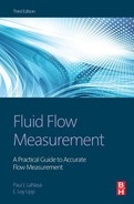
The first two systems designed on these basic concepts were the Pitot (1732) and the Venturi (1797). The flow nozzle was used in the late 1800s, and the orifice appeared in commercial use in the early 1900s. In each of these cases, the original investigators set their own requirements of design configuration, calculation, installation, and operation of their units. Continued research on and use of the various head devices since this early work has resulted in updated standards for their construction, installation, operation, and maintenance. Research continues today, reflecting the continued interest in the differential meter as a useful flow metering device (Figure 11-1).

The head device consists of a primary element that restricts the flowing stream, resulting in a pressure difference (pressure drop) across the primary element. This differential pressure relates to the flow rate through the restriction by application of Bernoulli’s equation. However, use of the equation assumes the physical area through the restriction to be the flow area through the restriction—and this is not the case with differential head meters where the physical area through the meter is always greater than the effective flow area. Bernoulli’s equation must therefore be adjusted to account for the difference in areas. The adjustment, called the “coefficient of discharge,” is a function of the meter’s physical area, differential pressure tap location, and Reynolds number. It can be calculated from equations developed from empirical data on each differential head meter. It is very important to remember that to take advantage of a head meter’s calculable performance, based on its mechanical construction, these specifications must be known and followed. Any deviation from these requirements necessitates a flow calibration to determine specific relationships of pressure drop to flow rate.
The related secondary devices consist of a differential pressure measuring unit with connecting piping and other measuring units required to define the flowing variables of the fluid, such as pressure, temperature, and composition. The pressure and differential pressure transducer is often combined into a single unit.
The advantages of a head meter can generally be listed as follows:
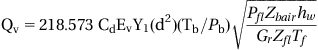
Specific head meters may not have all of the above advantages, but these are the general considerations for choosing a head meter. For example, the Venturi and the Pitot meters have relatively low permanent pressure losses. Others, such as the orifice, are adaptable to capacity changes by changing plates, provided the capacity change is not rapid with time. The Venturi and the nozzle will handle dirty fluids but they are not easily removed for maintenance (Figure 11-2).

Head devices have few application limitations and are used for most types of fluid flow measurement. They have been particularly applied in the measurement of water, natural gas, hydrocarbons of all kinds, chemicals, etc. It is easier to list the fluids where they are not used, such as viscous liquids, slurries, pulsating, multiphase, and non-Newtonian. Even these limits can be handled with special care under some circumstances.
In summary, the head devices cover a large category of flow meters in service today. Their wide acceptance and use is based on successful applications and service over many years.
Orifice Meter
Construction of the orifice meter is extremely important, since its mechanical construction defines its calibration under the various applicable standards. One of the most complete standards written on the orifice meter is the ANSI/API, Chapter 14, section 3, AGA Report No. 3, “Natural Gas Fluids Measurement,” more commonly called “AGA-3.”
AGA-3 is the bible of the orifice meter for gas meters. It represents the compilation of many different tests covering about 90 years with the latest agreed-upon knowledge of construction and installation, method of computing flow, orifice meter tables for natural gas, nomenclature and physical constants, and appendices. It is subject to periodic review and is updated as new knowledge is gained. It represents the most widely used standard for high pressure natural gas measurement and is successfully used commercially to measure the majority of the natural gas exchanged in the world.
Meter Design Changed
The following outline shows how an established standard can be changed because of new test results. All standards are living documents and must be continually followed to implement the improvements.
Detailed review is a must for the flow measurement practitioner. Depending on the words used, the part of the contract on the use of standards may state “The standard to be used is the latest edition of AGA-3,” or “The standard to be used is the latest edition of AGA-3 as mutually agreed upon,” or “The standard to be used is the [date] edition of AGA-3.”
Because of these variations, the use of the standard AGA-3 Part 2 is not universally used or understood. The basic contention of the standards is that these requirements must be met on all new installations or when an old station is reinstalled. The mechanical requirements of the meter tube description, fitting requirements, flow conditions, orifice plate requirements, and installation are the major sources of the changes listed below.
Meter Tube and Fitting
Orifice Plate
Flow Conditioner
Installation Requirements
Fluid dynamic conditions (further defined);
Plate eccentricity (tighter tolerances);
Plate perpendicularity (defined);
It is important that those knowledgeable in the practice of the standards recognize that the requirements have changed. To be in compliance with the new requirements, all of the changes must be made in new installations to obtain the uncertainty limits of the standard. Failure to do so may compromise the stations’ volumes. As time goes on it is expected that upgrading of the orifice standard will be continued. To take advantage of these new improvements, developments must be followed continually.
AGA-3 is also used to define an orifice installation for liquid flows. Its usefulness relates directly to understanding its contents. An introduction to the standard is given here, with the hope that this will form a basis for further study to properly complete the job of preparing system designers and users to measure with an orifice meter. The standard is based on a very large number of tests and the experiences of flow measurement practitioners; to use the report effectively, conditions found to be significant must be reproduced.
The basic premise of the standard is to make it unnecessary to calibrate each individual meter, but be able to predict and control its measurement accuracy by controlling how the meter is made and installed. This has been found possible to a tolerance acceptable for commercial measurement (custody transfer) for head devices.
The orifice is the most important and most widely used of the primary element head devices. It comes in many configurations for special applications, but by far the most common is the sharp-edged, concentric orifice plate using flange taps (located one inch from the upstream face of the plate and one inch from the downstream face of the orifice plate).
Reynolds numbers and beta ratios are the keys to the accuracy limits of plates. With a beta of roughly 0.10 to 0.75, the percent of uncertainty is 0.5% or less. However, at Reynolds numbers below 100,000 with large beta ratio (0.75), uncertainty is increased as shown in Table 11.1.
Table 11-1
Concentric sharp edged orifice plate coefficient of discharge uncertainty versus Reynolds number
| Reynolds Number | Uncertainty (%) |
| 100,000 | 0.58 |
| 50,000 | 0.59 |
| 10,000 | 0.70 |
| 5,000 | 0.84 |
| 4,000 | not recommended |
Uncertainty becomes so large—several percent—for Reynolds numbers below 4,000 that accurate measurement is no longer possible. The lowest Reynolds numbers typically occur on smaller runs with smaller plates on fluids more viscous than water.
An orifice used on liquid is limited by the lower pipe Reynolds numbers listed above, which are often more important because of the higher viscosities of liquids. The reason is the non-linearity of the flow coefficient with slight changes in the Reynolds number; at these low ranges, the changes in flow coefficient cause significant errors in flow rate measurement unless coefficient, volume, and Reynolds number calculations are iterated continually. For accurate measurement, rangeability of an orifice with a 100 inch recording device is usually limited to 3 to 1 for a single installation. However, multiple differential readout devices or multiple tubes are commonly used to extend the orifice rangeability.
The major orifice use is for general purpose, non-viscous flows where low cost is important. Compared to some other meters, it has a relatively high permanent pressure drop for a given flow rate, which may limit its use if pumping costs are a major consideration. Maintenance of the primary device consists of a periodic inspection and cleaning of the plate and the meter run, since inaccuracies can occur if initial equipment condition is not maintained. The primary advantages of the orifice use are its wide acceptance, simplicity, the large number of trained operating personnel available to maintain it, and the large amount of industry research data available on it.
The orifice standard is: ANSI/API 14.3/AGA-3 (latest edition). Its usefulness depends directly on how well the information in the standard is applied. Subjects covered by the standard include:
Part 1, General Equations and Uncertainty Guidelines
Part 2, Specification and Installation Requirements
Part 3, Natural Gas Applications
Part 4, Background, Developments, and Implementation Procedure and Subroutine Documentation for Empirical Flange-Tapped Discharge Coefficient Equation
Part 1 of the standard contains the basic flow equations for all fluids to be used to calculate flow rate through a concentric, square-edged, flange-tapped orifice meter. It provides an explanation of the terms used and methods for determining fluid properties. A definition of the uncertainty and guidelines for calculating possible errors in flow of fluids are given.
Part 2 of the standard was revised in April 2000 and gives specification and installation requirements for the manufacture and use of orifice plates, meter runs (upstream and downstream) orifice plate holders, pressure taps, thermometer wells, and flow conditioners. These specifications and requirements must be followed in detail to use the uncertainty calculations of Part 1. However, the standard recommends use of updated calculation methods, even if field equipment has not been updated to meet the new physical requirements. Variations from the requirements on initial installation, as well as during use of the station, will create the potential for error in flow measurement. In-place testing is required to determine what calibration factors should be applied, since the error estimates of the standard do not apply to non-standard metering situations.
Part 3 is specific to the use of the standard for natural gas measurement as practiced in North America.
Part 4 discusses the background, development, and limitations of the coefficient of discharge data. This material is of academic interest but not required to apply the data. However, the second section of Part 4 is important because example calculations detail the procedures to implement the data. The purpose of this section is to minimize accounting differences obtained by various computers and/or programs in using the data.
The latest version of the new document is different from previous standards in some details, such as the equations used and the requirements for manufacturing and installing an orifice. A grandfather clause allows stations under previous standards to continue to be used. The new standard contains the latest, most defensible data, and it reduces the uncertainty of measurement over a wider range of application of the orifice for flow measurement.
Other standards that cover the use of orifices include ISO 5167 and ASME MFC-3M. Since both trace back to the same basic databases, there are similarities between the documents. However, there are also differences that must be understood, since an orifice built to one standard may not meet the other standards.
The measurement fraternity is attempting to resolve these differences. In the meantime, if a specific standard must be met, then it must be specified in ordering and operating equipment.
Orifice Meter Description
An orifice meter consists of an orifice plate, a holding device, upstream downstream meter piping, and pressure taps. By far the most critical part of the meter is the orifice plate, particularly the widely used square-edged concentric plate, whose construction requirements are well documented in standards such as AGA-3 and ISO 5167-1. These standards define the plate’s edge, flatness, thickness—with bevel details, if required—and bore limitations.
The most common holding system is a pair of orifice flanges. However, for more precise measurement, various fittings are used. These simplify plate installation/removal for changing flow ranges and for easy inspection. In every case, the orifice must be installed concentric with the pipe within limits stated by the standard.
An orifice plate installed without specified upstream and downstream lengths of pipe controlled to close tolerances and/or without properly made pressure taps (usually flange) is not a “legitimate” flow meter; it must have specific tests run to determine its calibration. Since this is not economical, almost all orifice systems are built to meet the standard(s). This allows calculations to be made with specified tolerances. Control over orifice metering accuracy derives directly from data in the standard, which must be followed without exception.
Sizing
Sizing an orifice depends on the flow measurement task to be done. For example, a simple design would be a single meter tube with a single orifice plate in the mid beta ratio range, which would be sufficient for a fairly constant flow. However, if the flow grows over time, then sizing should allow for this growth by using a 0.20 beta plate. If flow is likely to decrease with time, then a large beta (such as 0.60) should be used. This way the meter tube size will not have to be changed in a short time period.
If continued growth is anticipated, an economical design would be to size the lengths and valves for the meter tube size slightly larger (i.e., if a 6 inch tube is chosen, sizing the meter tube length for an 8 inch tube, which could then replace the 6 inch without piping and header changes).
On non-custody transfer metering where utmost accuracy is not of prime importance, design betas can be changed to 0.15 and 0.70. If flow changes take place in a short time period, consideration should be given to several ranges for differential devices tied to one orifice or the use of multiple meter tubes switched in and out of service automatically. The differential chosen to size an orifice should not be full scale, but a reduced differential to allow for some inevitable variations. The amount of this reduction might be 10 to 20% of range depending on the likelihood of this much flow variation occurring.
Sizing of orifice stations is relatively simple for fluids with steady flow rates. Since a single orifice with a single readout system is limited to a flow range of roughly 3 to 1, for most accurate measurement, knowledge of the flow ranges is required to properly size the orifice to prevent over or under ranging. The controlling design flow rate should be the “normal flow” since the majority of the flow will, by definition, be at this rate. If the limits are beyond the 3-to-1 range, multiple orifice or readouts or possibly another meter should be chosen. There are many calculator and computer programs available in the industry to assist in this sizing. Likewise, manufacturers offer sizing calculations as part of their service of manufacturing plates.
Equations
The basic orifice meter mass flow equation in the common US system units (IP) is as follows:
(11.1)
Cd=orifice plate coefficient of discharge (dimensionless);
Ev=velocity of approach factor (dimensionless);
Y=expansion factor (dimensionless);
π=universal constant (3.14159);
d=orifice plate bore diameter calculated at flowing temperature Tf (feet);
gc=dimensional conversion constant (lbm-ft/lbf-sec2);
ρt,p=density of the fluid at flowing conditions (Pf, Tf) (lbm/ft3);
Note: The square root symbol (√) and engineering exponent 0.5 (Q0.5) are used interchangeably in this book.
In this equation qm is the mass flow rate and is the value to be determined.
Cd is the coefficient of discharge that has been empirically determined; it was last revised in the 1992 edition of the ANSI/API Chapter 14-3/AGA-3 documents. It depends on the plate and meter run size.
Ev, the velocity approach factor, corrects for the change in the flow constriction shape with various beta ratio plates—as well as differential pressure and pressure effects—as the flow goes from a meter run to the orifice restriction.
Y, the expansion factor, corrects for the change in density from the pressure tap to the orifice bore in gas measurement. It can be calculated from either an upstream or downstream tap depending on which measures the static pressure. Its value is a function of the beta ratio, differential pressure, static pressure at the designated tap, and the isentropic exponent of the flowing gas. The factor is unity for liquid flows.
π/4 is used to convert the orifice diameter to an area; d is the orifice plate diameter as determined by proper micrometer readings.
gc is a dimensional conversion constant.
ρt,p is the density of the fluid at flowing temperature and flowing pressure.
ΔP is the differential pressure measured across the orifice.
All values must be in a consistent set of units such as those shown above.
Most standards reduce the basic mass flow equation (Equation 11.1) into one that allows the more convenient use of mixed units and reduces constants to a single number. However, all versions trace back to this general basic equation (Equation 11.1).
Each standard and each differential device has equations that look different (notations are not the same), but they follow a basic relationship. The fundamental orifice meter mass flow equation in the various standards (presented in Chapter 2 and repeated here for your convenience) is written in various ways:
API 14.3, Sec 3, Part 1
(11.2)
AGA-3 1985
(11.3)
ISO 5167
(11.4)
ASME
(11.5)
 (11.5)
The equation may be simplified to use more easily measured variables (such as differential in inches of water rather than pounds per square inch), and some constants (such as π/4 and 2gc) may be reduced to numbers. If mixed units are used, corrections for these may also be included in the number. Details of this equation for each unit will be covered later in the appropriate section. Equation 11.1 can be converted to volume at base conditions by dividing the equation by the fluid density at base conditions:
(11.6)
Since flow measurement is often done with mixed units for convenience, the simplified equations contain a numerical constant for balancing the units. For example, in natural gas measurements, Equation 11.2 may be changed to:
(11.7)
 (11.7)
218.527=numerical constant and unit conversion factor;
Cd=orifice plate coefficient of discharge;
d=orifice plate bore diameter calculated at flowing temperature (Tf) (inches);
Gr=real gas relative density (specific gravity);
hw=orifice differential pressure in inches of water at 60°F;
Ev=velocity of approach factor;
Pfl=flowing pressure (upstream tap) (psia);
Y1=expansion factor (upstream tap);
Similar simplifications are also made in equations so applications are easier for standard units of the measured variables for liquid flows.
For these equations to be valid with minimum errors, the following factors are vital:
• The orifice plate and meter run must be kept clean and retain the original conditions specified by the standard.
• To ensure this, periodic inspection should be conducted to reaffirm conditions. Inspection frequency depends on problems of foreign material collection and possible damage. Inspections will confirm orifice diameter and thus the coefficient of discharge.
The expansion factor (Y1) for gas provides a relatively small correction for high pressure (above 100 psia) measurement provided the differential, in inches of water, is not allowed to exceed the static pressure (psia). As this ratio increases (below 100 psia), the correction factor increases, as does the error in the factor.
Flowing density can be measured directly with a densitometer that is periodically calibrated. It also may be calculated from appropriate equations of state whose accuracy must be established from the data upon which the equation is based. In either case, density is usually the second most important variable to determine in the equation.
The most important variable in the equation—the one that primarily determines flow measurement accuracy—is the differential pressure. Therefore, a major effort should be made to have as high a differential as possible (considering flowing conditions), and the best available differential transducers should be specified. Anything that can be done should be done to improve this most critical measurement factor. However, the most important term in the equation is the orifice bore, d. This is the only term that is squared. Therefore, small errors or mis-measurement of its value will significantly impact calculated flow.
Maintenance
(The following supplements information previously presented in Chapter 9.)
Orifice meter maintenance consists of periodic inspection (as indicated above), cleaning primary elements, and scheduled testing and calibration against standards (if necessary) of the secondary elements. Maintenance frequency, if not set by agreement or contract, should simply be based on experience and performed as often as necessary to correct any calibration drift or error that may occur. Proper records for each station will determine this schedule.
Advantages of the orifice meter:
1. Well documented in standards;
2. Enjoys wide acceptance; personnel knowledgeable across the industry about requirements for use and maintenance;
3. Relatively low cost to purchase and install;
4. No moving parts in the flow stream; and
5. When built to standards’ requirements, does not require calibration beyond confirming mechanical tolerances at the time of purchase and periodically in use.
Disadvantages of the orifice meter:
1. Low rangeability with a single device;
2. Relatively high pressure loss for a given flow rate, particularly at lower beta ratios;
3. More sensitive to flow disturbances at higher beta ratios than some meters; and
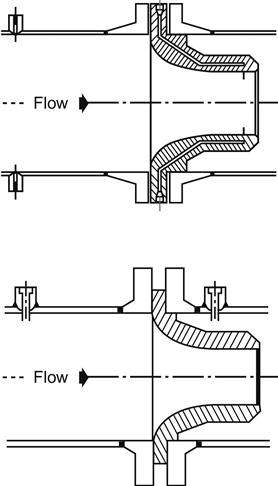
4. Flow pattern in the meter does not make meter self-cleaning (Figure 11-3).

Several special-shaped orifices for special applications are worthy of mention even though they are not in the industry’s standards. The quadrant-edge (quarter circle) orifice is used at Reynolds numbers below which the square-edge concentric orifice coefficient becomes too non-linear to be useful. A conic-entrance orifice can be used for a similar range of Reynolds number; however, it can be applied for even lower than quadrant-edged Reynolds numbers. Both of these devices should be used with limited diameter ratios, and the required flow rates and Reynolds numbers must be evaluated carefully to ensure good measurement. (See Chapter 6, Reference 5.)
Eccentric, segmental, and annular orifices—with accuracies in the order of 2%—are special devices to take care of dirty fluids and two-phase flows. Since these are not the best devices for obtaining accurate measurement, they are used only where these special conditions exist. No detailed standards exist for these devices. For details on construction of these orifices, see Chapter 6, Reference 5.
Honed flow sections are orifice runs made in sizes of 0.25 through 1.50 inches. They are covered by the ASME, and data are available from manufacturers who have developed special manufacturing requirements and special coefficients to calculate corrected flow. These devices are used for low flows of gas, liquid, and steam with a higher tolerance than standard-sized meter tubes of 2.00 inches and larger that are covered in the industry standards.
Flow Nozzles
Another important flow element is the flow nozzle. Several configurations are available, the most important of which are the ASME long radius nozzle, high or low beta series, and the throat tap nozzle for gas and liquid. In Europe, another nozzle shape outlined is the ISA-1932 that is used more often than the ASME nozzle. Both have the same rangeability limitation as orifices—approximately 3 to 1 for a 100 inch recorder. (See ASME MFC-3M and ASME PTC-6 for details of construction.)
When flow rates change with time and thus require nozzles to be changed, this is more difficult than changing an orifice plate. The nozzle, however, is better able to sweep suspended particles by the restriction because its contour is more streamlined than the orifice. The ability to handle particulates is particularly good if a nozzle is installed in the vertical position with flow downward.
Nozzles are used mostly for high-velocity, non-viscous, erosive fluid flows. However, they have considerable acceptance in certain industries, such as electrical power generation. Standard nozzles are moderately priced, but throat tap nozzles are very expensive. The throat tap nozzles provide some of the highest accuracies of all primary devices, since they are allowed in only a very limited beta ratio range of 0.45 to 0.55.
The special throat tap type is used primarily for accurate acceptance testing of electrical generating plants. This is a very expensive nozzle because it must be flow calibrated prior to use, and its calibration must meet the standard coefficient value within ±0.25%. This does not allow much room for error in manufacture or calibration. Because of these problems, its use is primarily restricted to the power industry, where the acceptance testing can justify the nozzle cost (Figure 11-4).
The devices are very difficult to remove for inspection and cleaning, and their use in fluids when deposits may build up is not recommended. Installation requirements for nozzles are similar to those for orifices. Requirements are detailed in the ASME documents previously listed.
The nozzle has mistakenly been said to have low pressure drop. But for a given differential and pipe size, it is better stated that a lower beta ratio can be used. At times, a smaller tube size can be used with the nozzle than with the orifice. Permanent pressure drops will be approximately equal for a given set of flow conditions for either device if the differential range is set. Nozzle sizing must be based on good flow data that is fairly stable because of its restricted range. The expense of incorrect sizing should always be kept in mind.
ASME nozzle taps are located in the pipe wall one pipe diameter upstream and one-half pipe diameter downstream. The ISA-1932 nozzle uses corner taps. Nozzles are usually mounted between pipe flanges.
Nozzles may be fitted with a diffuser cone to reduce the pressure loss by guiding flow back to the meter tube. It is possible to truncate this diffuser to approximately four times the nozzle throat diameter and have about as full recovery as with a cone extending to the wall.
The equation for the ASME (low or high beta) flow nozzle is in the same form as the orifice, with the ASME nozzle coefficient restricted to a Reynolds number of 10,000 or greater. The coefficient value is approximately 0.95 versus an orifice coefficient of approximately 0.60, so the nozzle handles over 50% more flow for a given size and differential reading. A special equation can be used for the coefficient at lower Reynolds numbers, but the change of coefficient in this range requires an iterative process of flow velocity and Reynolds number to maintain accuracy. Nozzles with other shapes may have different coefficient equations.
Operational accuracy of the nozzle is again directly related to the ability to measure at higher differentials because of the square root relationship with flow. It is best not to measure below 10 inches of differential, but higher differentials (400 to 800 inches of water, for example) can be used because of the mechanical strength of the nozzle versus the orifice.
The nozzle is best applied to clean fluids, since removal for cleaning is very difficult. Any change of nozzle throat finish has a direct effect on measurement accuracy. Where critical measurements are made, the installation must be capable of being shut down, or have a bypass to allow periodic inspection and cleaning. This increases the cost of a nozzle installation. For the most part, nozzles usually receive very little maintenance.
1. Can be used at higher velocities with little damage to the nozzle surface, which allows using smaller sized meters for a given flow; and
2. Throat tap nozzles have the lowest stated uncertainty tolerances of all head devices, but require calibration to prove and have restricted beta ratio ranges.
Venturi Meters
Low pressure drop devices are headed in the United States by the classical Venturi, which is used for liquid, gas, and steam at pipe Reynolds numbers of 100,000 and over. Venturi rangeability, like an orifice meter, is dependent on the differential readout and is 3 to 1 for a single 100 inch range recorder. Venturis are mainly used to measure liquids, clean or dirty.
The Dall tube is popular in the United Kingdom as a low-pressure device for these same measurements (Figure 11-5).

Where low pressure drops are required in non-viscous fluids, the pressure drop depends on the angle of the downstream cone and the beta ratio of the Venturi. Venturis have the disadvantage that their size makes inspection and changing cumbersome. It is recommended that an initial calibration be run for precision measurement, since they tend to be more difficult to manufacture precisely than a nozzle or an orifice. These problems can be secondary to the savings achieved in the costs of low operating pressure drops.
The classical (Herschel) Venturi is built to specifications of the ASME MFC-3M and ISO-5167 with an angled inlet and exit cone on a cylindrical throat section. It is designed to minimize pressure drop and to be somewhat self-cleaning, since there are no sharp corners in the flowing stream where materials may collect. Venturis have an overall length of approximately eight diameters; this makes them unwieldy to make, install, and remove for inspection. The actual design has several options that must be chosen before the length and shape dimensions are set. One sometimes overlooked is inlet cone finish, which affects coefficient limits. Each Venturi is unique, and consequently the volumes to be measured must be accurately known, because once a Venturi is built, there is no flexibility for change of design flow rates in the unit.
Venturi Installation
Installation requirements for piping depend upon the upstream fitting (i.e., elbows, valves, reducers, and expanders) but are generally shorter than for a nozzle or orifice with the same beta ratio. No straightening vanes are required by the standards. However, experience shows that no swirl can be tolerated coming into a Venturi, so two elbows in different planes or pinched valves should not be installed in upstream piping, since they tend to create swirl.
In summary, Venturis are 3-to-1 flow range devices with a single 100 inch manometer recorder. Their throughput has the highest efficiency of any of the head devices with an approximate coefficient of 0.98. They should be designed to the actual conditions of flow with no design allowance for errors, thus the flow specifications must be correct.
The flow equation is the same as for the orifice previously covered except for the coefficient of discharge. A Venturi should perform correctly over time provided the surface of the inlet cone and the throat are not changed by corrosion, erosion, or deposits. Venturis can be cleaned if provision is made to remove the unit from service for maintenance. Other than this (which is seldom done), most maintenance consists of work with the secondary equipment.
Other low loss devices are the Universal Venturi and the LoLoss tube.
Advantages of Venturis (and other low loss head devices):
1. Limited rangeability; must be used only on installations where the flow rate is well known and varies less than 3 to 1.
2. Very expensive; should be flow calibrated to provide accuracy in the range of ±1.00%; and
3. Units are big and weigh more than comparable head devices; this makes them difficult to install and inspect.
Other Head Meters
Pitot tubes (standard and averaging) can be covered in a single section since they are similar in their application limitations. They are used for measurement of liquids and gas. The meters do not “look” at the total flow profile, and their accuracies relate to how well the readings represent average velocity. When line velocity at a single point is measured, accuracy is generally no better than ±5% unless specific calibrations are run (Figure 11-6).

Over limited ranges, these devices are used for control purposes rather than custody transfer. Their major advantages are that they create practically no pressure drop and are inexpensive. On the other hand, velocities in normal pipeline designs are such that measured differentials in Pitots (which may be a maximum of 8 inches of water differential) limit application to fairly steady rates of flow (low rangeability). These very inexpensive devices may be installed so they can be removed for maintenance without stopping line flow.
Disadvantages of Pitot meters:
1. Point velocity measured is assumed to represent full pipeline average velocity, which limits accuracy unless the flow profile is closely controlled; and
2. For normal pipeline velocities, the indicated differential is very low, which makes its accuracy poor and its rangeability very limited.
Elbow Meters
As fluid flows around an elbow, centrifugal force makes the pressure on the outside wall higher than the pressure on the inside wall. This pressure difference is proportional to flow, and its coefficient can be estimated from a knowledge of the elbow dimensions. For more accurate measurement, an elbow (with at least ten diameters of straight pipe upstream—straightening vanes are recommended to stabilize swirling flow—and five diameters downstream) should be flow calibrated. If welds on an inlet elbow and pressure taps are carefully made, elbows will calibrate with a very stable calibration curve.
These units, however, are more often used for flow control (high repeatability) rather than for accurate flow measurement. Piping systems already have elbows present, and their use as a meter adds no pressure loss not already present. But normal pipeline velocities do not generate differentials (normal maximum about 9 inches), and this limits accuracy and severely limits rangeability (Figure 11-7).

Elbows are normally used for control with stable flow rates where repeatability is more important than absolute values of flow.