Search in book...
Toggle Font Controls
Create new playlist

Name your new playlist

Playlist description (optional)
Sign In

Email address

Password

Forgot Password?

or

Continue with Facebook

Continue with Google
Sign Up

Full Name

Email address

Confirm Email Address

Password

or

Continue with Facebook

Continue with Google

Basic Flow Measurement Laws

The chapter goes through the laws which should be recognized and obeyed before flow measurement is attempted. Certain physical laws explain what happens in the “real” world. Some of these laws explain what happens when fluid flows in a pipeline, and these in turn explain what happens to a flowing stream as it goes through a meter. The laws discussed in this chapter include the law of “conservation of mass”, also called the “Law of Continuity,” the law of “conservation of energy”, the Fluid Friction Law and the fundamental flow equation. The Reynolds number is explained, as are the gas laws and ways to correct for the effects of temperature and pressure.

Keywords

physical law; fluid flow; conservation of mass; conservation of energy; fluid friction law; fundamental flow equation; Reynolds number

All of the following laws should be recognized and obeyed before flow measurement is attempted. Certain physical laws explain what happens in the “real” world. Some of these laws explain what happens when fluid flows in a pipeline, and these in turn explain what happens to a flowing stream as it goes through a meter. All variables in the equations must be in consistent units of measurement.

The law of “conservation of mass” states that the mass rate is constant. In other words, the amount of fluid moving through a meter is neither added to nor taken from as it progresses from point 1 to point 2 (Figure 2-1). This is also called the “Law of Continuity,” and it can be written mathematically as follows:

$M_{1} = M_{2}$ $M_{1} = M_{2}$ (2.1)

(2.1)

where:

M₁=mass rate upstream;

M₂=mass rate downstream.

Figure 2-1 The amount of fluid flowing is constant at points 1 and 2.

Since mass rate equals fluid density multiplied by pipe area multiplied by fluid velocity, Equation 2.1 can be rewritten as:

$ρ_{1} A_{1} V_{1} = ρ_{2} A_{2} V_{2}$ $ρ_{1} A_{1} V_{1} = ρ_{2} A_{2} V_{2}$ (2.2)

(2.2)

where:

ρ=fluid density at a designated point in the pipe;

A=pipe area at the designated point;

V=average velocity in the pipe at the designated point;

_{1, 2}=upstream and downstream positions.

In terms of volume rate this can be restated as:

$Q = A V$ $Q = A V$ (2.3)

(2.3)

where:

Q=volume per unit time at flowing conditions;

A, V=as previously defined.

The law of “conservation of energy” states that all energy entering a system at point 1 is also in the system at point 2, even though one form of energy may be exchanged for another. (Note: the Bernoulli theorem relates the same physics in fluid mechanics.) The total energy in a system is made up of several types:

1. Potential Energy due to the fluid position or pressure.

2. Flow Work Energy required for the fluid to flow. The fluid immediately preceding that between point 1 and point 2 must be at a slightly higher pressure in order to exert a force on the volume between 1 and 2, so that this will flow.

3. Kinetic Energy (energy of motion) due to fluid velocity.

4. Internal Energy due to fluid temperature and chemical composition.

5. External Energy is energy exchanged with the fluid existing between point 1 and point 2 and its surroundings. These are normally heat and work energies.

The Fluid Friction Law states that energy is required to overcome friction and move fluid from point 1 to point 2. For the purpose of calculating flows, certain assumptions are made about the stability of the system energy under steady flow. The main energy concerns are the potential and kinetic energies (definitions 1 and 3); the others are either of no importance, do not change between position 1 and position 2, do not occur, or are taken care of by calibration procedures. A generalized statement of this energy balance is given below:

$K E_{1} + P E_{1} = K E_{2} + P E_{2}$ $K E_{1} + P E_{1} = K E_{2} + P E_{2}$ (2.4)

(2.4)

Kinetic energy (KE) is energy of motion (velocity). Potential energy (PE) is energy of position (pressure).

In simple terms, this equation can be rewritten:

${PE}_{1} + {VE}_{1} = {PE}_{2} + {VE}_{2}$ ${PE}_{1} + {VE}_{1} = {PE}_{2} + {VE}_{2}$ (2.5)

(2.5)

where:

PE=pressure energy;

VE=velocity energy.

Equation 2.5 is the “ideal flow equation” for a restriction in a pipe. In real applications, however, certain corrections are necessary. The major equation correction is an efficiency factor called the “coefficient of discharge.” This factor takes into account the difference between the ideal and the real world. The ideal equation states that 100% of the flow will pass an orifice with a given differential, when in fact empirical tests indicate that a lower fraction of the flow actually passes for a given differential—for example, about 60% with differential between flange taps on an orifice meter, 95% across a nozzle, and 98% across a Venturi (Figure 2-2). This is caused by the device’s inefficiency or the loss from inefficiency caused by turbulence at the device where energy of pressure is not all converted to energy of motion. This factor has been determined by industry studies over the years and is reported as a “discharge coefficient.”

Figure 2-2 Orifice, flow nozzle, and Venturi meters all have permanent pressure losses somewhat less than 100% of full measurement differential; an ultrasonic meter is like an open section of pipe (non-intrusive) with no additional permanent pressure drop.

Equations 2.4 and 2.5 assume no energy, such as heat, is added or removed from the stream between upstream and the meter itself. This is normally of small concern unless there is significant difference between the flowing and ambient temperatures (i.e., steam measurement), or when measuring a fluid whose volume is sensitive to very small temperature changes, such as near its critical temperature. (Three common examples are ethylene, carbon dioxide gas, and hot water near its boiling point.)

It is also assumed that no temperature change is caused by fluid expansion (because of the lower pressure in the meter) from the upstream pressure to the meter. The small pressure difference between the two locations normally makes this theoretical consideration insignificant. If there is a change in state (i.e., from liquid to gas or gas to liquid) then this “insignificant” temperature change is no longer insignificant. Furthermore, the volume occupied (assuming no mass holdup) is much greater in the gaseous phase than the liquid phase; volume ratios of gas to liquids are as much as several hundred for some common fluids. Because of these problems, flow measurement of flashing liquids or condensing gases should not be attempted.

Reynolds Number

The Reynolds number is a useful tool for relating how a meter will react to a variation in fluids from gases to liquids. Since an impossible amount of research would be required to test every meter on every fluid we wish to measure, it is desirable that a relationship between fluid factors be known. Reynolds’ work in 1883 defines these relationships through his Reynolds number, which is defined by the equation:

$Re = \frac{ρ Dv}{µ}$ $Re = \frac{ρ Dv}{µ}$ (2.6)

(2.6)

where:

Re=Reynolds number, a dimensionless number;

ρ=density of the fluid;

D=diameter of the passage way;

v=velocity of the fluid;

μ=viscosity of the fluid.

Note: All parameters are given in the same units, so that when multiplied together they all cancel out, and the Reynolds number has no units. Units in the pound, foot, second system are shown below:

Re=no units;

ρ=#/cubic feet;

D=feet;

v=feet/sec;

μ=#/foot-sec.

Based on Reynolds’ work, the flow profile (which affects all velocity-sensitive meters and some linear meters) has several important values. At values of 2,000 and below, the flow profile is bullet-shaped (parabolic). Between 2,000 and 4,000 the flow is in the transition region. At 4,000 and above the flow is in the turbulent flow area and the profiles are fairly flat. Thus, calculation of the Reynolds number will define the flow velocity pattern and approximate limits of the meter’s application. To completely define the meter’s application there must be no deformed profiles, such as after an elbow or where upstream piping has imparted swirl to the stream.

These effects will be further discussed in the sections covering the description and application of different meters, in Chapters 8, 9, and 10, and the equations will be covered more thoroughly later in this book.

These equations can be combined and rewritten in simplified forms. However, it is important to recognize the assumptions which have been made, so that if a metering situation deviates from what has been assumed, a “flag will go up” to indicate that the effect of Reynolds number must be evaluated and treated.

Gas Laws

Gas properties are almost always measured at conditions other than standard or base conditions, so the measured values must be converted by calculation, using the gas laws, to those at the desired base conditions, to make the values comparable.

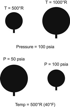
Boyle’s Law states that the volume of a gas is inversely proportional to its pressure for an ideal gas at constant temperature (Figure 2-3).

$V = Constant / P$ $V = Constant / P$ (2.7)

(2.7)

where:

V=volume;

P=pressure.

Figure 2-3 Diagrammatic representation of Boyle’s Law, showing that volume is inversely proportional to pressure.

Charles’ Law states that the volume of a gas is directly proportional to its temperature for an ideal gas at constant pressure (Figure 2-4).

$V = Constant / T$ $V = Constant / T$ (2.8)

(2.8)

Figure 2-4 Diagrammatic representation of Charles’ Law, showing that volume is proportional to temperature.

The Ideal Gas Law combines Boyle’s and Charles’ laws; it can be written:

$\frac{V_{b}}{V_{f}} = \frac{P_{f} T_{b}}{P_{b} T_{f}}$ $\frac{V_{b}}{V_{f}} = \frac{P_{f} T_{b}}{P_{b} T_{f}}$ (2.9)

(2.9)

where:

_b=base conditions;

_f=flowing conditions.

The Real Gas Law (non-ideal) corrects for the fact that gases do not follow the ideal law at conditions of high pressure and/or low temperature (Figures 2-5 to 2-7). The Ideal Gas Law equation must be corrected to:

$\frac{V_{b}}{V_{f}} = \frac{P_{f} T_{b} Z_{b}}{P_{b} T_{f} Z_{f}}$ $\frac{V_{b}}{V_{f}} = \frac{P_{f} T_{b} Z_{b}}{P_{b} T_{f} Z_{f}}$ (2.10)

(2.10)

Figure 2-5 The Ideal Gas Law combines Boyle’s and Charles’ laws.

Figure 2-6 Ideal and actual conditions depart at extremes of pressure and temperature.

Figure 2-7 Gas-filled balloons also illustrate pressure/temperature/volume relationships.

where:

Z is the compressibility correction.

Empirically derived values for various gases are available in industry standards or can be predicted from correlations based on their critical temperatures and critical pressures.

Expansion of Liquids

Like gases, liquid volumes vary with temperature and pressure. Because liquids have little compressibility with pressure, this effect is often ignored unless temperatures approach the critical temperature (within 20%). The effects of temperature are not as large in liquids as they are in gases (Figure 2-8). If there is a large difference between the flowing and base temperatures or flowing and base pressures, or if a high degree of accuracy is desired, then a correction should be made.

Figure 2-8 Effect of temperature on liquid volume.

The temperature-effect correction is based on cubical expansion for each liquid as follows:

$V_{b} = V_{f} [1 + B (T_{f} - T_{b})]$ $V_{b} = V_{f} [1 + B (T_{f} - T_{b})]$ (2.11)

(2.11)

where:

B=the coefficient of cubical expansion of the liquid;

V=volume;

T=temperature;

_b=base;

_f=flowing.

The pressure-effect correction is based on compressibility effects for each liquid (this follows API procedures):

$(\frac{1}{1 - [P - (P_{e} - P_{b})] F})$ $(\frac{1}{1 - [P - (P_{e} - P_{b})] F})$ (2.12)

(2.12)

where:

P=pressure;

_b=base, absolute;

_e=equilibrium vapor, absolute;

_f=flowing, absolute;

F=liquid compressibility correction factor.

If P_b=P_e, then:

$V_{b} = V_{f} .$ $V_{b} = V_{f} .$

The specific equations for head meters and linear meters will be covered in more detail in the chapters which discuss them (Chapters 11 and 12).

Fundamental Flow Equation

The fundamental flow equation for differential devices is:

$q_{m} = \frac{C E_{v} Y π d^{2}}{4} \sqrt{2 g_{c} ρ_{f} Δ P}$ $q_{m} = \frac{C E_{v} Y π d^{2}}{4} \sqrt{2 g_{c} ρ_{f} Δ P}$ (2.13)

(2.13)

where:

q=mass flow rate;

C=discharge coefficient of flow at the Reynolds number for the device in question;

Y=expansion factor (usually assumed to be 1.0 for liquids);

π=pi;

d=restriction diameter at flowing conditions;

g_c=dimensional conversion constant;

ρ_f=density of flowing fluid;

ΔP=difference in pressure during flow caused by the restriction;

E_v=velocity of approach factor.

(Note: Discharge coefficient values are available for specific restrictions with specific sets of pressure taps.)

Each standard and each differential device has equations that look different (notations are not the same), but they follow a basic relationship. The fundamental orifice meter mass flow equations in the various standards are:

API 14.3, Sec 3, Part 1

$q_{m} = C_{d} E_{v} Y d^{2} (π / 4) \sqrt{2 g_{c} ρ_{t p} Δ P}$ $q_{m} = C_{d} E_{v} Y d^{2} (π / 4) \sqrt{2 g_{c} ρ_{t p} Δ P}$ (2.14)

(2.14)

AGA-3 1985

$q_{m} = K Y_{1} d^{2} (π / 4) \sqrt{2 g_{c} ρ_{t p} Δ P}$ $q_{m} = K Y_{1} d^{2} (π / 4) \sqrt{2 g_{c} ρ_{t p} Δ P}$ (2.15)

(2.15)

ISO 5167

$q_{m} = C E ε d^{2} (π / 4) \sqrt{2 Δ P ρ}$ $q_{m} = C E ε d^{2} (π / 4) \sqrt{2 Δ P ρ}$ (2.16)

(2.16)

ASME

$q_{m} = (π / 4) C ε^{2} \sqrt{\frac{2 Δ P ρ}{1 - β^{4}}}$ $q_{m} = (π / 4) C ε^{2} \sqrt{\frac{2 Δ P ρ}{1 - β^{4}}}$ (2.17)

(2.17)

In these equations:

$C = C_{d}$ $C = C_{d}$

$E_{v} = E = {[1 / (1 - β^{4})]}^{0.5}$ $E_{v} = E = {[1 / (1 - β^{4})]}^{0.5}$

$Y = ɛ$ $Y = ɛ$

$2 Δ P = {2g}_{c} Δ p$ $2 Δ P = {2g}_{c} Δ p$

$K = C_{d} E_{v} = CE = C / {[1 / (1 - β^{4})]}^{0.5}$ $K = C_{d} E_{v} = CE = C / {[1 / (1 - β^{4})]}^{0.5}$

The equation may be simplified to involve more easily measured variables (such as differential in inches of water rather than pounds per square inch), and some constants (such as π⁴ and 2g_c) may be reduced to numbers. If mixed units are used, corrections for these may also be included in the number. Details of this equation for each unit will be covered later in the appropriate section.

The “volume flow rate” may be derived from the mass flow:

$q_{b} = \frac{q_{m}}{ρ_{b}}$ $q_{b} = \frac{q_{m}}{ρ_{b}}$ (2.18)

(2.18)

where:

q_b=volume flow rate at base conditions;

q_m=mass flow rate;

ρ_b=density of fluid at base conditions.

Equations for non-head type volume meters are simpler since they basically reduce the volume determined by the meter under flowing conditions to that under base conditions, as was discussed in the section above on basic laws.

$q_{f} F_{b} = q_{b}$ $q_{f} F_{b} = q_{b}$ (2.19)

(2.19)

where:

q_f=volume at flowing conditions;

F_b=factor to reduce from flowing to base (corrects for effects of compressibility, pressure, and temperature);

q_b=volume at base conditions.

If the meter measures mass, then there is no reduction to base required (a pound is a pound the world around!) and:

$q_{mf} = q_{mb}$ $q_{mf} = q_{mb}$ (2.20)

(2.20)

where:

q_mf=mass at flowing conditions;

q_mb=mass at base conditions.

..................Content has been hidden....................

You can't read the all page of ebook, please click here login for view all page.

Table of Contents for 2. Basic Flow Measurement Laws

Create new playlist

Sign In

Sign Up

Basic Flow Measurement Laws

Keywords

Reynolds Number

Gas Laws

Expansion of Liquids

Fundamental Flow Equation

Table of Contents for
2. Basic Flow Measurement Laws