Chapter 7

Maintaining Multiple Worksheets

In This Chapter

Moving from sheet to sheet in your workbook

Adding and deleting sheets in a workbook

Selecting sheets for group editing

Naming sheet tabs descriptively

Rearranging sheets in a workbook

Displaying parts of different sheets

Comparing two worksheets side by side

Copying or moving sheets from one workbook to another

Creating formulas that span different worksheets

When you’re brand new to spreadsheets, you have enough trouble keeping track of a single worksheet and the very thought of working with more than one may be a little more than you can take. However, after you get a little experience under your belt, you’ll find that working with more than one worksheet in a workbook is no more taxing than working with just a single worksheet.

Don’t confuse the term workbook with worksheet. The workbook forms the document (file) that you open and save while you work. Each workbook (file) normally contains a single blank worksheet, to which you can add as many worksheets as you need by clicking the New Sheet button on the Status bar (the one with plus sign in a circle). Multiple worksheets in a single workbook act like the loose-leaf pages in a notebook binder; you can add or remove sheets as needed. To help you keep track of the worksheets in your workbook and navigate between them, Excel provides sheet tabs (Sheet1, Sheet 2, and Sheet3) that are like the tab dividers in a loose-leaf notebook.

Juggling Multiple Worksheets

You need to understand how to work with more than one worksheet in a workbook, but it’s also important to understand why you’d want to do such a crazy thing in the first place. The most common situation is, of course, when you have a bunch of worksheets that are related to each other and, therefore, naturally belong together in the same workbook. For example, consider the case of Mother Goose Enterprises with its different companies: Jack Sprat Diet Centers, Jack and Jill Trauma Centers, Mother Hubbard Dog Goodies; Rub-a-Dub-Dub Hot Tubs and Spas; Georgie Porgie Pudding Pies; Hickory, Dickory, Dock Clock Repair; Little Bo Peep Pet Detectives; Simple Simon Pie Shoppes; and Jack Be Nimble Candlesticks. To keep track of the annual sales for all these companies, you could create a workbook containing a worksheet for each of the nine different companies.

By keeping the sales figures for each company in a different sheet of the same workbook, you gain all the following benefits:

You can enter the stuff that’s needed in all the sales worksheets (if you select those sheet tabs) just by typing it once into the first worksheet (see the section “Editing en masse,” later in this chapter).

In order to help you build the worksheet for the first company’s sales, you can attach macros to the current workbook so that they are readily available when you create the worksheets for the other companies. (A macro is a sequence of frequently performed, repetitive tasks and calculations that you record for easy playback — see Chapter 12 for details.)

You can quickly compare the sales of one company with the sales of another (see the section “Opening Windows on Your Worksheets,” later in this chapter).

You can print all the sales information for each company as a single report in one printing operation. (Read Chapter 5 for specifics on printing an entire workbook or particular worksheets in a workbook.)

You can easily create charts that compare certain sales data from different worksheets (see Chapter 10 for details).

You can easily set up a summary worksheet with formulas that total the quarterly and annual sales for all nine companies (see the upcoming “Summing Stuff on Different Worksheets” section).

Sliding between the sheets

Each blank workbook that you open contains a single worksheet given the prosaic name, Sheet1. To add more sheets to your workbook, you simply click the New Sheet button on the Status bar (the one with plus sign in a circle). Each worksheet you add with the New Sheet command button is assigned a generic Sheet name with the next available number appended to it, so if you click this button twice in a new workbook containing Sheet1, Excel adds Sheet2 and Sheet3. These worksheet names appear on tabs at the bottom of the workbook window.

To go from one worksheet to another, you simply click the tab that contains the name of the sheet you want to see. Excel then brings that worksheet to the top of the stack, displaying its information in the current workbook window. You can always tell which worksheet is current because its name is in bold type on the tab and its tab appears as an extension of the current worksheet with a bold line appearing along the bottom edge.

The only problem with moving to a new sheet by clicking its sheet tab occurs when you add so many worksheets to a workbook (as I describe in the upcoming section “Don’t Short-Sheet Me!”) that not all the sheet tabs are visible at any one time, and the sheet tab you want to click is not visible in the workbook indicated on the Status bar by an ellipsis (three periods in a row) that appears immediately after the last visible sheet tab.

To deal with the problem of not having all the sheet tabs visible, Excel provides two tab scrolling buttons on the Status bar before the first sheet tab that you can use to bring new sheet tabs into view:

Click the Next tab scroll button (with the triangle pointing right) to bring the next unseen tab of the sheet on the right into view. Hold down the Shift key while you click this button to scroll several tabs at a time. Hold down the Ctrl key while you click this button to bring the last group of sheets, including the last sheet tab into view.

Click the Previous tab scroll button (with the triangle pointing left) to bring the next unseen tab of the sheet on the left into view. Hold down the Shift key while you click this button to scroll several tabs at a time. Hold down the Ctrl key when you click this button to bring the first group of sheet tabs, including the very first tab, into view.

Right-click either tab scroll button to open the Activate dialog box (shown in Figure 7-1) showing a list of all the worksheets — to activate a worksheet in this list, select it followed by OK.

Figure 7-1: Right-click a tab scroll button to display the Activate dialog box with a list of all the worksheets in your workbook.

---

---

Just don’t forget that scrolling the sheet tab into view is not the same thing as selecting it: You still need to click the tab for the desired sheet to bring it to the front of the stack (or select it in the Activate dialog box shown in Figure 7-1).

To make it easier to find the sheet tab you want to select without having to do an inordinate amount of tab scrolling, drag the tab split bar (the three vertical dots that immediately follow the New Sheet button) to the right. Doing this reveals more sheet tabs on the Status bar, consequently making the horizontal scroll bar shorter. If you don’t care at all about using the horizontal scroll bar, you can maximize the number of sheet tabs in view by actually getting rid of this scroll bar. To do this, drag the tab split bar to the right until it’s smack up against the vertical split bar.

When you want to restore the horizontal scroll bar to its normal length, you can either manually drag the tab split bar to the left or simply double-click it.

Editing en masse

Each time you click a sheet tab, you select that worksheet and make it active, enabling you to make whatever changes are necessary to its cells. You may encounter times, however, when you want to select bunches of worksheets so that you can make the same editing changes to all of them simultaneously. When you select multiple worksheets, any editing change that you make to the current worksheet — such as entering information in cells or deleting stuff from them — affects the same cells in all the selected sheets in exactly the same way.

Suppose you need to set up a new workbook with three worksheets that contain the names of the months across row 3 beginning in column B. Prior to entering January in cell B3 and using the AutoFill handle (as described in Chapter 2) to fill in the 11 months across row 3, you select all three worksheets (Sheet1, Sheet2, and Sheet3, for argument’s sake). When you enter the names of the months in the third row of the first sheet, Excel will insert the names of the months in row 3 of all three selected worksheets. (Pretty slick, huh?)

Likewise, suppose you have another workbook in which you need to get rid of Sheet2 and Sheet3. Instead of clicking Sheet2, clicking Home⇒Delete⇒Delete Sheet on the Ribbon or pressing Alt+HDS, and then clicking Sheet3 and repeating the Delete Sheet command, select both worksheets and then zap them out of existence in one fell swoop by clicking Home⇒Delete⇒Delete Sheet on the Ribbon or pressing Alt+HDS.

To select a bunch of worksheets in a workbook, you have the following choices:

To select a group of neighboring worksheets, click the first sheet tab and then scroll the sheet tabs until you see the tab of the last worksheet you want to select. Hold the Shift key while you click the last sheet tab to select all the tabs in between — the old Shift-click method applied to worksheet tabs.

To select a group of non-neighboring worksheets, click the first sheet tab and then hold down the Ctrl key while you click the tabs of the other sheets you want to select.

To select all the sheets in the workbook, right-click the tab of the worksheet that you want active and choose Select All Sheets from the shortcut menu that appears.

Excel shows you worksheets that you select by turning their sheet tabs white (although only the active sheet’s tab name appears in bold) and displaying [Group] after the filename of the workbook on the Excel window’s title bar.

To deselect the group of worksheets when you finish your group editing, you simply click a nonselected (that is, grayed out) worksheet tab. You can also deselect all the selected worksheets other than the one you want active by right-clicking the tab of the sheet you want displayed in the workbook window and then clicking Ungroup Sheets on its shortcut menu.

Don’t Short-Sheet Me!

For some of you, the single worksheet automatically put into each new workbook that you start is as much as you would ever, ever need (or want) to use. For others of you, a measly, single blank worksheet might seldom, if ever, be sufficient for the type of spreadsheets you create (for example, suppose that your company operates in 10 locations, or you routinely create budgets for 20 different departments or track expenses for 40 account representatives).

Excel 2013 makes it a snap to insert additional worksheets in a workbook (up to 255 total) — simply click the Insert Worksheet button that appears to the immediate right of the last sheet tab.

To insert a bunch of new worksheets in a row in the workbook, select a group with the same number of tabs as the number of new worksheets you want to add, starting with the tab where you want to insert the new worksheets. Next, click Home⇒Insert⇒Insert Sheet on the Ribbon or press Alt+HIS.

To delete a worksheet from the workbook, follow these steps:

1. Click the tab of the worksheet that you want to delete.

2. Choose Home⇒Delete⇒Delete Sheet on the Ribbon, press Alt+HDS, or right-click the tab and choose Delete from its shortcut menu.

If the sheet you’re deleting contains any data, Excel displays a scary message in an alert box about how you’re going to delete the selected sheets permanently.

3. Go ahead and click the Delete button or press Enter if you’re sure that you won’t be losing any data you need when Excel zaps the entire sheet.

This is one of those situations where Undo is powerless to put things right by restoring the deleted sheet to the workbook.

To delete a bunch of worksheets from the workbook, select all the worksheets you want to delete and then choose Home⇒Delete⇒Delete Sheet, press Alt+HDS, or choose Delete from the tab’s shortcut menu. Then, when you’re sure that none of the worksheets will be missed, click the Delete button or press Enter when the alert dialog box appears.

If you find yourself constantly adding a bunch of new worksheets, you may want to think about changing the default number of worksheets so that the next time you open a new workbook, you have a more realistic number of sheets on hand. To change the default number, choose File⇒Options or press Alt+FT to open the General tab of the Excel Options dialog box. Enter a new number between 1 and 255 in the Include This Many Sheets text box in the When Creating New Workbooks section or select a new number with the spinner buttons before you click OK.

A worksheet by any other name . . .

The sheet names that Excel comes up with for the tabs in a workbook (Sheet1, Sheet2, Sheet3) are, to put it mildly, not very original — and are certainly not descriptive of their function in life! Luckily, you can easily rename a worksheet tab to whatever helps you remember what you put on the worksheet (provided this descriptive name is no longer than 31 characters).

---

---

To rename a worksheet tab, just follow these steps:

1. Double-click the sheet tab or right-click the sheet tab and then click Rename on its shortcut menu.

The current name on the sheet tab appears selected.

2. Replace the current name on the sheet tab by typing the new sheet name.

3. Press Enter.

Excel displays the new sheet name on its tab at the bottom of the workbook window.

A sheet tab by any other color . . .

In Excel 2013, you can assign colors to the different worksheet tabs. This feature enables you to color-code different worksheets. For example, you could assign red to the tabs of those worksheets that need immediate checking and blue to the tabs of those sheets that you’ve already checked.

To assign a color to a worksheet tab, right-click the tab and highlight Tab Color on its shortcut menu to open a submenu containing the Tab Color pop-up palette. Then, click the new color for the tab by clicking its color square on the color palette. After you select a new color for a sheet tab, the name of the active sheet tab appears underlined in the color you just selected. When you make another sheet tab active, the entire tab takes on the assigned color (and the text of the tab name changes to white if the selected color is sufficiently dark enough that black lettering is impossible to read).

To remove a color from a tab, right-click the sheet tab and highlight the Tab Color option to open the Tab Color pop-up palette. Then, click No Color at the bottom of the Tab Color palette.

Getting your sheets in order

Sometimes, you may find that you need to change the order in which the sheets appear in the workbook. Excel makes this possible by letting you drag the tab of the sheet you want to arrange in the workbook to the place where you want to insert it. While you drag the tab, the mouse or Touch Pointer changes to a sheet icon with an arrowhead on it, and the program marks your progress among the sheet tabs (see Figures 7-2 and 7-3 for examples). When you release the mouse button, Excel reorders the worksheets in the workbook by inserting the sheet at the place where you dropped the tab off.

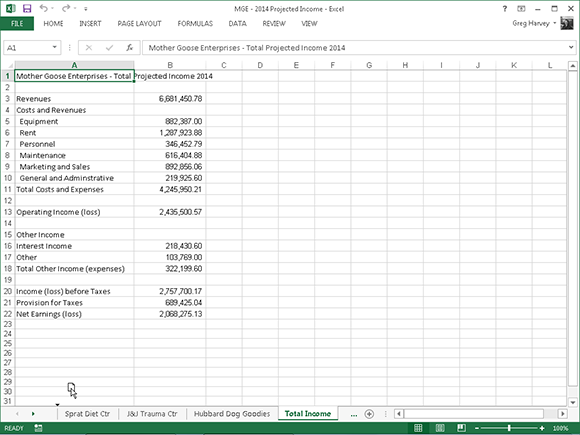
Figure 7-2: Drag the Total Income tab to the front to reorder the sheets in this worksheet.

Figure 7-3: The relocated Total Income sheet is now at the front of the workbook.

If you hold down the Ctrl key while you drag the sheet tab icon, Excel inserts a copy of the worksheet at the place where you release the mouse button. You can tell that Excel is copying the sheet rather than just moving it in the workbook because the pointer shows a plus sign (+) on the sheet tab icon containing the arrowhead. When you release the mouse button or remove your finger or stylus, Excel inserts the copy in the workbook, which is designated by the addition of (2) after the tab name.

For example, if you copy Sheet5 to another place in the workbook, the sheet tab of the copy is named Sheet5 (2). You can then rename the tab to something civilized (see the earlier section “A worksheet by any other name . . .” for details).

You can also move or copy worksheets from one part of a workbook to another by activating the sheet that you want to move or copy and then choosing Move or Copy on its shortcut menu. In the Before Sheet list box in the Move or Copy dialog box, click the name of the worksheet in front of which you want the active sheet moved or copied.

To move the active sheet immediately ahead of the sheet you select in the Before Sheet list box, simply click OK. To copy the active sheet, be sure to select the Create a Copy check box before you click OK. If you copy a worksheet instead of just moving it, Excel adds a number to the sheet name. For example, if you copy a sheet named Total Income, Excel automatically names the copy of the worksheet Total Income (2), which appears on its sheet tab.

Opening Windows on Your Worksheets

Just as you can split a single worksheet into panes so that you can view and compare different parts of that same sheet on the screen (see Chapter 6), you can split a single workbook into worksheet windows and then arrange the windows so that you can view different parts of each worksheet on the screen.

To open the worksheets that you want to compare in different windows, you simply insert new workbook windows (in addition to the one that Excel automatically opens when you open the workbook file itself) and then select the worksheet that you want to display in the new window. You can accomplish this with the following steps:

1. Click the New Window command button on the View tab or press Alt+WN to create a second worksheet window; then click the tab of the worksheet that you want to display in this second window (indicated by the :2 that Excel adds to the end of the filename in the title bar).

2. Click the New Window command button or press Alt+WN again to create a third worksheet window; then click the tab of the worksheet that you want to display in this third window (indicated by the :3 that Excel adds to the end of the filename in the title bar).

3. Continue clicking the New Window command button or pressing Alt+WN to create a new window and then selecting the tab of the worksheet you want to display in that window for each worksheet you want to compare.

4. Click the Arrange All command button on the View tab or press Alt+WA and select one of the Arrange options in the Arrange Windows dialog box (as I describe next); then click OK or press Enter.

When you open the Arrange Windows dialog box, you’re presented with the following options:

Tiled: Select this button to have Excel arrange and size the windows so that they all fit side by side on the screen. (Check out Figure 7-4 to see the screen that appears after you choose the Tiled button to organize four worksheet windows.)

Horizontal: Select this button to have Excel size the windows equally and place them one above the other. (In Figure 7-5, you can see the screen that appears after you choose the Horizontal button to organize these four worksheet windows.)

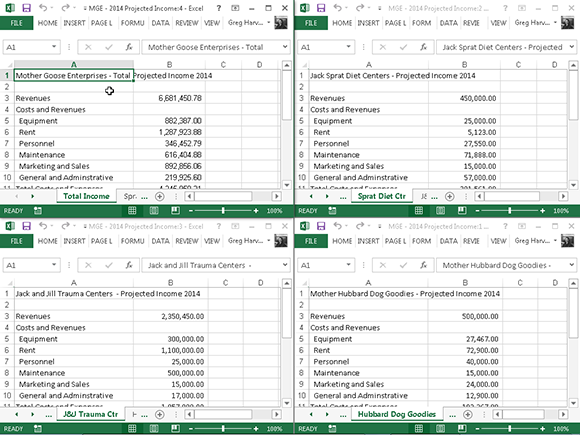
Figure 7-4: Four worksheet windows arranged with the Tiled option.

Figure 7-5: Four worksheet windows with the Horizontal option.

Vertical: Select this button to have Excel size the windows equally and place them next to each other. (Look at Figure 7-6 to see the screen that appears after you choose the Vertical option to arrange four worksheet windows.)

Cascade: Select this button to have Excel arrange and size the windows so that they overlap one another with only their title bars showing. (See Figure 7-7 for the screen that appears after you select the Cascade option to arrange four worksheet windows.)

Windows of Active Workbook: Select this check box to have Excel show only the windows that you have open in the current workbook. Otherwise, Excel also displays all the windows in any other workbooks you have open. Yes, it is possible to open more than one workbook — as well as more than one window within each open workbook — provided that the device you’re running Excel on has sufficient screen space and memory, and you have enough stamina to keep track of all that information.

Figure 7-6: Four worksheet windows arranged with the Vertical option.

After you place windows in one arrangement or another, activate the one you want to use (if it isn’t selected already) by clicking it in the Excel program window. Alternatively, you position the mouse or Touch Pointer on the Excel 2013 program icon on the Windows 7 or 8 taskbar to display pop-up thumbnails for each of the worksheet windows you have open. To display the contents of one of the Excel worksheet windows without the others visible, highlight its pop-up thumbnail on the Windows taskbar. To then activate a particular worksheet window from the taskbar, you simply click its thumbnail.

When you click a worksheet window that has been tiled or placed in the horizontal or vertical arrangement, Excel indicates that the window is selected simply by displaying the cell pointer around the active cell and highlighting that cell’s column and row heading in the worksheet. When you click the title bar of a worksheet window you place in the cascade arrangement, the program displays the window on the top of the stack, as well as displaying the cell pointer in the sheet’s active cell.

Figure 7-7: Four worksheet windows arranged with the Cascade option.

You can temporarily zoom the window to full size by clicking the Maximize button on the window’s title bar. When you finish your work in the full-size worksheet window, return it to its previous arrangement by clicking the window’s Restore button.

To select the next tiled, horizontal, or vertical window on the screen or display the next window in a cascade arrangement with the keyboard, press Ctrl+F6. To select the previous tiled, horizontal, or vertical window or to display the previous window in a cascade arrangement, press Ctrl+Shift+F6. These keystrokes work to select the next and previous worksheet window even when the windows are maximized in the Excel program window.

If you close one of the windows by clicking Close (the X in the upper-right corner) or by pressing Ctrl+W, Excel doesn’t automatically resize the other open windows to fill in the gap. Likewise, if you create another window by clicking the New Window command button on the View tab, Excel doesn’t automatically arrange it in with the others. (In fact, the new window just sits on top of the other open windows.)

To fill in the gap created by closing a window or to integrate a newly opened window into the current arrangement, click the Arrange command button to open the Arrange Windows dialog box and click OK or press Enter. (The button you selected last time is still selected; if you want to choose a new arrangement, select a new button before you click OK.)

Don’t try to close a particular worksheet window by choosing File⇒Close or by pressing Alt+FC because you’ll only succeed in closing the entire workbook file, getting rid of all the worksheet windows you created!

When you save your workbook, Excel saves the current window arrangement as part of the file along with all the rest of the changes. If you don’t want to save the current window arrangement, close all but one of the windows (by clicking their Close buttons or selecting their windows and then pressing Ctrl+W). Then click that last window’s Maximize button and select the tab of the worksheet that you want to display the next time you open the workbook before saving the file.

Comparing Worksheets Side by Side

You can use the View Side by Side command button (the one with the picture of two sheets side by side like tiny tablets of the Ten Commandments) on the Ribbon’s View tab to quickly and easily do a side-by-side comparison of any two worksheet windows that you have open. When you click this button (or press Alt+WB after opening two windows), Excel automatically tiles them horizontally (as though you had selected the Horizontal option in the Arrange Windows dialog box), as shown in Figure 7-8.

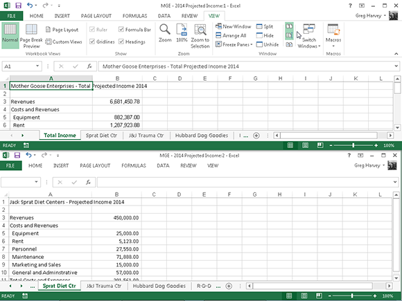
Figure 7-8: Comparing two worksheet windows side by side.

If you have more than two windows open at the time you click the View Side by Side command button (Alt+WB), Excel opens the Compare Side by Side dialog box where you click the name of the window that you want to compare with the one that’s active at the time you choose the command. As soon as you click OK in the Compare Side by Side dialog box, Excel horizontally tiles the active window above the one you just selected.

Immediately below the View Side by Side command button in the Window group of the View tab on the Ribbon, you find the following two command buttons, which are useful when comparing windows side by side:

Synchronous Scrolling: When this command button is selected (as it is by default), any scrolling that you do in the worksheet in the active window is mirrored and synchronized in the worksheet in the inactive window beneath it. To be able to scroll the worksheet in the active window independently of the inactive window, click the Synchronous Scrolling button to deselect it.

Reset Window Position: Click this command button after you manually resize the active window (by dragging its size box or an edge of the window) to restore the two windows to their previous side-by-side arrangement.

Shifting Sheets to Other Workbooks

In some situations, you need to move a particular worksheet or copy it from one workbook to another. To move or copy worksheets between workbooks, follow these steps:

1. Open both the workbook with the worksheet(s) that you want to move or copy and the workbook that is to contain the moved or copied worksheet(s).

Choose File⇒Open or press Ctrl+O to open both the workbooks.

2. Select the workbook that contains the worksheet(s) that you want to move or copy.

To select the workbook with the sheet(s) to move or copy, click its pop-up thumbnail on the Windows taskbar.

3. Select the worksheet(s) that you want to move or copy.

To select a single worksheet, click its sheet tab. To select a group of neighboring sheets, click the first tab and then hold down Shift while you click the last tab. To select various nonadjacent sheets, click the first tab and then hold down Ctrl while you click each of the other sheet tabs.

4. Right-click its sheet tab and then click Move or Copy on its shortcut menu.

Excel opens up the Move or Copy dialog box (similar to the one shown in Figure 7-9) in which you indicate whether you want to move or copy the selected sheet(s) and where to move or copy them.

5. In the To Book drop-down list box, select the name of the workbook to which you want to copy or move the worksheets.

If you want to move or copy the selected worksheet(s) to a new workbook rather than to an existing one that you have open, select the (new book) option that appears at the very top of the To Book drop-down list.

6. In the Before Sheet list box, select the name of the sheet that the worksheet(s) you’re about to move or copy should precede. If you want the sheet(s) that you’re moving or copying to appear at the end of the workbook, choose the (Move to End) option.

7. Select the Create a Copy check box to copy the selected worksheet(s) to the designated workbook (rather than move them).

8. Click OK or press Enter to complete the move or copy operation.

Figure 7-9: Use the Move or Copy dialog box to move or copy from the current workbook into a different workbook.

If you prefer a more direct approach, you can move or copy sheets between open workbooks by dragging the sheet tabs from one workbook window to another. This method works with several sheets or a single sheet; just be sure that you select all the sheet tabs before you begin the drag-and-drop procedure.

To drag a worksheet from one workbook to another, you must open both workbooks. Click the Arrange All command button on the View tab or press Alt+WA and then select an arrangement (such as Horizontal or Vertical to put the workbook windows either on top of each other or side by side). Before you close the Arrange Windows dialog box, be sure that the Windows of Active Workbook check box is not selected; that is, does not contain a check mark.

After arranging the workbook windows, drag the worksheet tab from one workbook to another. If you want to copy rather than move the worksheet, hold down the Ctrl key while you drag the sheet icon(s). To locate the worksheet in the new workbook, position the downward-pointing triangle that moves with the sheet icon in front of the worksheet tab where you want to insert it; then release the mouse button or remove your finger or stylus from the touchscreen.

This drag-and-drop operation is one of those that you can’t reverse by using Excel’s Undo feature (see Chapter 4). This means that if you drop the sheet in the wrong workbook, you’ll have to go get the wayward sheet yourself and then drag and drop it into the place where it once belonged!

In Figures 7-10 and 7-11, I show how easy it is to move or copy a worksheet from one workbook to another using this drag-and-drop method.

In Figure 7-10, you see two workbook windows: the Book1 new workbook (left pane) and the MGE – 2014 Projected Income workbook (right pane). I arranged these workbook windows with the View Side by Side command button on the View tab. To copy the Sprat Diet Ctr sheet from the MGE – 2014 Projected Income workbook to the new Book1 workbook, I simply select the Sprat Diet Ctr sheet tab, hold down the Ctrl key, and drag the sheet icon to its new position before Sheet1 of the Book1 workbook.

Now look at Figure 7-11 to see the workbooks after I release the mouse button. As you can see, Excel inserts the copy of the Sprat Diet Ctr worksheet into the Book1 workbook at the place indicated by the triangle that accompanies the sheet icon (before Sheet1 in this example).

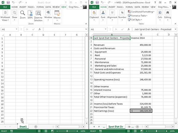
Figure 7-10: Copying the Sprat Diet Ctr worksheet to the Book1 workbook via drag and drop.

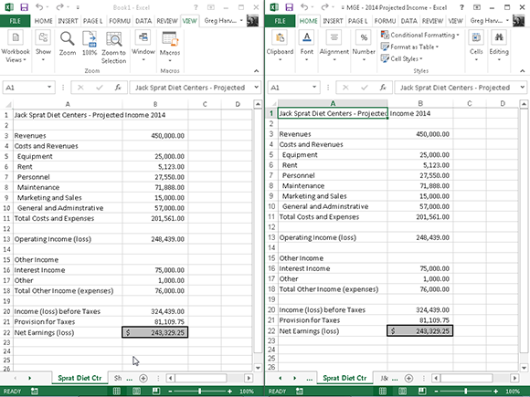
Figure 7-11: Book1 workbook after moving a copy of the Sprat Diet Ctr before Sheet1.

Summing Stuff on Different Worksheets

I’d be remiss if I didn’t introduce you to the fascinating subject of creating a summary worksheet that recaps or totals the values stored in a bunch of other worksheets in the workbook.

The best way that I can show you how to create a summary worksheet is to walk you through the procedure of making one (entitled Total Projected Income) for the MGE – 2014 Projected Income workbook. This summary worksheet totals the projected revenue and expenses for all the companies that Mother Goose Enterprises operates.

Because the MGE – 2014 Projected Income workbook already contains nine worksheets with the 2014 projected revenue and expenses for each one of these companies, and because these worksheets are all laid out in the same arrangement, creating this summary worksheet will be a breeze:

1. I insert a new worksheet in front of the other worksheets in the MGE – 2014 Projected Income workbook and rename its sheet tab from Sheet1 to Total Income.

To find out how to insert a new worksheet, refer to this chapter’s “Don’t Short-Sheet Me!” section. To find out how to rename a sheet tab, read the earlier “A worksheet by any other name . . .” section.

2. Next, I enter the worksheet title Mother Goose Enterprises – Total Projected Income 2014 in cell A1.

Do this by selecting cell A1 and then typing the text.

3. Finally, I copy the rest of the row headings for column A (containing the revenue and expense descriptions) from the Sprat Diet Ctr worksheet to the Total Income worksheet.

To do this, select cell A3 in the Total Income sheet and then click the Sprat Diet Ctr tab. Select the cell range A3:A22 in this sheet; then press Ctrl+C, click the Total Income tab again, and press Enter.

I am now ready to create the master SUM formula that totals the revenues of all nine companies in cell B3 of the Total Income sheet:

1. I start by clicking cell B3 and pressing Alt+= to select the AutoSum feature.

Excel then puts =SUM( ) in the cell with the insertion point placed between the two parentheses.

2. I click the Sprat Diet Ctr sheet tab, and then click its cell B3 to select the projected revenues for the Jack Sprat Diet Centers.

The Formula bar reads =SUM(‘Sprat Diet Ctr’!B3) after selecting this cell.

3. Next, I type a comma (,) — the comma starts a new argument. I click the J&J Trauma Ctr sheet tab and then click its cell B3 to select projected revenues for the Jack and Jill Trauma Centers.

The Formula bar now reads =SUM(‘Sprat Diet Ctr’!B3,‘J&J Trauma Ctr’!B3) after I select this cell.

4. I continue in this manner, typing a comma (to start a new argument) and then selecting cell B3 with the projected revenues for all the other companies in the following seven sheets.

At the end of this procedure, the Formula bar now appears with the whopping SUM formula shown on the Formula bar in Figure 7-12.

5. To complete the SUM formula in cell B3 of the Total Income worksheet, I then click the Enter box in the Formula bar (I could press Enter on my keyboard, as well).

In Figure 7-12, note the result in cell B3. As you can see in the Formula bar, the master SUM formula that returns 6,681,450.78 to cell B3 of the Total Income worksheet gets its result by summing the values in B3 in all nine of the supporting worksheets.

Figure 7-12: The Total Income worksheet after I create a SUM formula to total projected revenues for all the Mother Goose companies.

If you want to select the same cell across multiple worksheets, you can press and hold the Shift key, and then select the last worksheet. All worksheets in between the first and last will be included in the selection, or in this case, the calculation.

All that’s left to do now is to use AutoFill to copy the master formula in cell B3 down to row 22 as follows:

1. With cell B3 still selected, I drag the AutoFill handle in the lower-right corner of cell B3 down to cell B22 to copy the formula for summing the values for the nine companies down this column.

2. Then I delete the SUM formulas from cells B4, B12, B14, B15, and B19 (all of which contain zeros because these cells have no income or expenses to total).

In Figure 7-13, you see the first section of the summary Total Income worksheet after I copy the formula created in cell B3 and after I delete the formulas from the cells that should be blank (all those that came up 0 in column B).

Figure 7-13: The Total Income worksheet after I copy the SUM formula and delete formulas that return zero values.