Chapter 4

Going Through Changes

In This Chapter

Opening workbook files for editing

Undoing your boo-boos

Moving and copying with drag and drop

Copying formulas

Moving and copying with Cut, Copy, and Paste

Deleting cell entries

Deleting and inserting columns and rows

Spell-checking the worksheet

Corroborating cell entries with the Text to Speech feature

Picture this: You just finished creating, formatting, and printing a major project with Excel — a workbook with your department’s budget for the next fiscal year. Because you finally understand a little bit about how the Excel thing works, you finish the job in crack time. You’re actually ahead of schedule.

You turn the workbook over to your boss so that she can check the numbers. With plenty of time for making those inevitable last-minute corrections, you’re feeling on top of this situation.

Then comes the reality check — your boss brings the document back, and she’s plainly agitated. “We forgot to include the estimates for the temps and our overtime hours. They go right here. While you’re adding them, can you move these rows of figures up and those columns over?”

As she continues to suggest improvements, your heart begins to sink. These modifications are in a different league than, “Let’s change these column headings from bold to italic and add shading to that row of totals.” Clearly, you’re looking at a lot more work on this baby than you had contemplated. Even worse, you’re looking at making structural changes that threaten to unravel the very fabric of your beautiful worksheet.

As the preceding fable points out, editing a worksheet in a workbook can occur on different levels:

You can make changes that affect the contents of the cells, such as copying a row of column headings or moving a table to a new area in a particular worksheet.

You can make changes that affect the structure of a worksheet itself, such as inserting new columns or rows (so that you can enter new data originally left out) or deleting unnecessary columns or rows from an existing table so that you don’t leave any gaps.

You can even make changes to the number of worksheets in a workbook (by either adding or deleting sheets).

In this chapter, you discover how to make these types of changes safely to a workbook. As you see, the mechanics of copying and moving data or inserting and deleting rows are simple to master. It’s the impact that such actions have on the worksheet that takes a little more effort to understand. Not to worry! You always have the Undo feature to fall back on for those (hopefully rare) times when you make a little tiny change that throws an entire worksheet into complete and utter chaos.

In the final section of this chapter (“Eliminating Errors with Text to Speech”), you find out how to use the Text to Speech feature to check out and confirm the accuracy of the data entries you make in your worksheets. With Text to Speech, you can listen to your computer read back a series of cell entries while you visually corroborate their accuracy from the original source document. Text to Speech can make this sort of routine and otherwise labor-intensive editing much easier and greatly increase the accuracy of your spreadsheets.

Opening Your Workbooks for Editing

Before you can do any damage — I mean, make any changes — in a workbook, you have to open it up in Excel. To open a workbook from within Excel, you can choose File⇒Open, press Alt+FO, or use the old standby keyboard shortcuts Ctrl+O or Ctrl+F12.

When you use the Ctrl+F12 shortcut, as opposed to any of the other methods for opening a workbook, Excel 2013 bypasses the Open screen and takes you directly to the Open dialog box. This is fine provided that the workbook file you need to work with is in the currently open folder (by default, this is the Documents folder in the Libraries folder on your local hard drive, unless you’ve opened files from another folder and drive during your work session).

If you’ve just launched Excel 2013 and don’t yet have any workbooks open, you can open the workbook for editing by selecting it on the list of files under the Recent heading displayed in the left pane of the Start screen. If the file you want to edit is not in this list, click the Open Other Workbooks link at the bottom of this left pane to have Excel take you to the Open screen.

Opening files in the Open screen

When the Open screen is first displayed in the Excel 2013 Backstage (shown in Figure 4-1) the Recent Workbooks option in the Places pane on the left is selected. If the file you want to open isn’t shown in this list in the right-hand pane, you need to select one of the other Places options:

Windows Live’s SkyDrive to open a workbook file that’s saved in the cloud in one of your folders on your Windows Live SkyDrive (for more information on SkyDrive or to open an account, visit http://windows.microsoft.com/en-US/skydrive/home). When you select this option, the right-hand pane lists folders on your SkyDrive that you accessed recently as well as Browse button that enables to locate other folders in the Open dialog box.

Computer to a workbook file saved locally on your computer’s hard drive or a network drive to which you have access. When you select this option, the right-hand pane lists folders on your local and network drives that you accessed recently, as well as a Documents (meaning the Documents folder in the library under your user name on the hard drive), Desktop (the Windows 7 or 8 Desktop), and Browse button that enables to locate workbook files in their respective folder in the Open dialog box.

Add a Place to designate add access to a SharePoint site or your SkyDrive account. When you select this option, the right-hand pane contains an Office365 SharePoint and SkyDrive button. Click the Office365 SharePoint button to log into a SharePoint site for which you have a user ID and password to add its folders to the Open screen under the Computer option. Select the SkyDrive option to log into your Windows Live account (for which you have a user ID and password) to add your space in the cloud to the Open screen under the Windows Live’s SkyDrive option.

Figure 4-1: Use the SkyDrive option in the Open screen to open an online workbook file for editing.

Operating the Open dialog box

After you select a folder and drive in the Excel 2013 Open screen or press the Ctrl+F12 shortcut from within Excel, the program displays an Open dialog box similar to the one shown in Figure 4-2. The Open dialog box is divided into panes: the Navigation pane on the left, where you can select a new folder to open, and the main pane on the right showing the icons for all the subfolders in the current folder, as well as the documents that Excel can open.

The folder with contents displayed in the Open dialog box is either the one designated as the Default File Location on the Save tab of the Excel Options dialog box, the folder you last opened during your current Excel work session, or the folder you selected in the Open screen of the Backstage view.

To open a workbook in another folder, click its link in the Favorite Links section of the Navigation pane or click the Expand Folders button (the one with the triangle pointing upward) and click its folder in this list.

If you open a new folder and it appears empty of all files (and you know that it’s not an empty folder), this just means the folder doesn’t contain any of the types of files that Excel can open directly (such as workbooks, template files, and macro sheets). To display all the files, whether or not Excel can open them directly (meaning without some sort of conversion), click the drop-down button that appears next to the drop-down list box that currently displays All Excel Files and then click All Files on its drop-down menu.

Figure 4-2: Selecting the workbook file to open for editing in Excel in the Open dialog box.

When the icon for the workbook file you want to work with appears in the Open dialog box, you can then open it either by clicking its file icon and then clicking the Open button or, if you’re handy with the mouse, by just double-clicking the file icon.

You can use the slider attached to the Change Your View drop-down list button in the Open dialog box to change the way folder and file icons appear in the dialog box. When you select Large Icons or Extra Large Icons on this slider (or anywhere in between), the Excel workbook icons actually show a preview of the data in the upper-left corner of the first worksheet when the file is saved with the preview picture option turned on:

To enable the preview feature when saving workbooks in Excel 2013, select the Save Thumbnail check box in the Save As dialog box before saving the file for the first time.

To enable the preview feature when saving workbooks in Excel 97 through 2003, click the Save Preview Picture check box on the Summary tab of the workbook’s Properties dialog box (File⇒Properties) before saving the file for the first time.

This preview of part of the first sheet can help you quickly identify the workbook you want to open for editing or printing.

Changing the Recent files settings

Excel 2013 automatically keeps a running list of the last 25 files you opened in the Recent Workbooks list on the Open screen when the Recent Workbooks option is selected under Places. If you want, you can have Excel display more or fewer files in this list.

To change the number of recently opened files that appear, follow these simple steps:

1. Choose File⇒Options⇒Advanced or press Alt+FTA to open the Advanced tab of the Excel Options dialog box.

2. Type a new entry (between 1 and 50) in the Show This Number of Recent Documents text box located in the Display section or use the spinner buttons to increase or decrease this number.

3. Click OK or press Enter to close the Excel Options dialog box.

If you don’t want any files displayed in the Recent Workbooks list, either on the Excel or Open screen in the Backstage view, enter 0 in the Show This Number of Recent Documents text box or select it with the spinner buttons.

Select the Quickly Access This Number of Recent Workbooks check box on the Advanced tab of the Excel Options dialog box (right below the Show This Number of Recent Workbooks option) to have Excel display the four most recently opened workbooks as menu items at the bottom of the File menu in the Backstage view. That way, you can open any of them by clicking its button even when the Open screen is not displayed in the Backstage view. If four workbook files is too many or not sufficient, you can decrease or increase the number of files shown at the bottom of the File menu by replacing 4 in the text box that appears to the right of the Quickly Access This Number of Recent Workbooks check box option.

Opening multiple workbooks

If you know that you’re going to edit more than one of the workbook files shown in the list box of the Open dialog box, you can select multiple files in the list box, and Excel will then open all of them (in the order they’re listed) when you click the Open button or press Enter.

Remember that in order to select multiple files that appear sequentially in the Open dialog box, you click the first filename and then hold down the Shift key while you click the last filename. To select files that aren’t listed sequentially, you need to hold down the Ctrl key while you click the various filenames.

After the workbook files are open in Excel, you can then switch documents by clicking their filename buttons on the Windows taskbar or by using the Flip feature (Alt+Tab) to select the workbook’s thumbnail. (See Chapter 7 for detailed information on working on more than one worksheet at a time.)

Find workbook files

The only problem you can encounter in opening a document from the Open dialog box is locating the filename. Everything’s hunky-dory as long as you can see the workbook filename listed in the Open dialog box or know which folder to open in order to display it. But what about those times when a file seems to migrate mysteriously and can’t be found on your computer?

For those times, you need to use the Search Documents text box in the upper-right corner of the Open dialog box. To find a missing workbook, click this search text box and then begin typing characters used in the workbook’s filename or contained in the workbook itself.

As soon as Windows finds any matches for the characters you type, the names of the workbook files (and other Excel files, such as templates and macro sheets) appear in the Open dialog box. When the workbook you want to open is listed, you can open it by clicking its icon and filename followed by the Open button, or by double-clicking it.

Using the Open file options

The drop-down button attached to the Open command button at the bottom of the Open dialog box enables you to open the selected workbook file(s) in a special way, including:

Open Read-Only: This command opens the files you select in the Open dialog box’s list box in a read-only state, which means that you can look but you can’t touch. (Actually, you can touch; you just can’t save your changes.) To save changes in a read-only file, you must use the Save As command (File⇒Save As or Alt+FA) and give the workbook file a new filename. (Refer to Chapter 2.)

Open as Copy: This command opens a copy of the files you select in the Open dialog box. Use this method of opening files as a safety net: If you mess up the copies, you always have the originals to fall back on.

Open in Browser: This command opens workbook files you save as web pages (which I describe in Chapter 12) in your favorite web browser. This command isn’t available unless the program identifies that the selected file or files were saved as web pages rather than plain old Excel workbook files.

Open in Protected View: This command opens the workbook file in Protected View mode that keeps you from making any changes to the contents of its worksheets until you click the Enable Editing button that appears in the orange Protected View panel at the top of the screen.

Open and Repair: This command attempts to repair corrupted workbook files before opening them in Excel. When you select this command, a dialog box appears giving you a choice between attempting to repair the corrupted file or opening the recovered version, extracting data from the corrupted file, and placing it in a new workbook (which you can save with the Save command). Click the Repair button to attempt to recover and open the file. Click the Extract Data button if you tried unsuccessfully to have Excel repair the file.

Much Ado about Undo

Before you start tearing into the workbook that you just opened, get to know the Undo feature, including how it can put right many of the things that you could inadvertently mess up. The Undo command button on the Quick Access toolbar is a regular chameleon button. When you delete the cell selection by pressing the Delete key, the Undo button’s ScreenTip reads Undo Clear (Ctrl+Z). If you move some entries to a new part of the worksheet by dragging it, the Undo command button ScreenTip changes to Undo Drag and Drop (Ctrl+Z).

In addition to clicking the Undo command button (in whatever guise it appears), you can also choose this command by pressing Ctrl+Z (perhaps for unZap).

The Undo command button on the Quick Access toolbar changes in response to whatever action you just took; that is, it changes after each action. If you forget to strike when the iron is hot, so to speak, and don’t use the Undo feature to restore the worksheet to its previous state before you choose another command, you then need to consult the drop-down menu on the Undo button. Click its drop-down button that appears to the right of the Undo icon (the curved arrow pointing to the left). After the Undo drop-down menu appears, click the action on this menu that you want undone. Excel will then undo this action and all actions that precede it in the list (which are selected automatically).

Undo is Redo the second time around

After using the Undo command button on the Quick Access toolbar, Excel 2013 activates the Redo command button to its immediate right. If you delete an entry from a cell by pressing the Delete key and then click the Undo command button or press Ctrl+Z, the ScreenTip that appears when you position the mouse pointer over the Redo command button reads Redo Clear (Ctrl+Y).

When you click the Redo command button or press Ctrl+Y, Excel redoes the thing you just undid. Actually, this sounds more complicated than it is. It simply means that you use Undo to switch between the result of an action and the state of the worksheet just before that action until you decide how you want the worksheet (or until the cleaning crew turns off the lights and locks up the building).

What to do when you can’t Undo?

Just when you think it is safe to begin gutting the company’s most important workbook, I really feel that I have to tell you that (yikes!) Undo doesn’t work all the time! Although you can undo your latest erroneous cell deletion, bad move, or unwise copy, you can’t undo your latest rash save. (You know, like when you meant to choose Save As from the File menu in the Backstage view to save the edited worksheet under a different document name but chose Save and ended up saving the changes as part of the current document.)

Unfortunately, Excel doesn’t let you know when you are about to take a step from which there is no return — until it’s too late. After you’ve gone and done the un-undoable and you click the Undo button where you expect its ScreenTip to say Undo blah, blah, it now reads Can’t Undo.

One exception to this rule is when the program gives you advance warning (which you should heed). When you choose a command that is normally possible but because you’re low on memory or the change will affect so much of the worksheet, or both, Excel knows that it can’t undo the change if it goes through with it, the program displays an alert box telling you that there isn’t enough memory to undo this action and asking whether you want to go ahead anyway. If you click the Yes button and complete the edit, just realize that you do so without any possibility of pardon. If you find out, too late, that you deleted a row of essential formulas (that you forgot about because you couldn’t see them), you can’t bring them back with Undo. In such a case, you would have to close the file (File⇒Close) and NOT save your changes.

Doing the Old Drag-and-Drop Thing

The first editing technique you need to learn is drag and drop. As the name implies, you can use this technique to pick up a cell selection and drop it into a new place on the worksheet. Although drag and drop is primarily a technique for moving cell entries around a worksheet, you can adapt it to copy a cell selection, as well.

To use drag and drop to move a range of cell entries (one cell range at a time), follow these steps:

1. Select a cell range.

2. Position the mouse pointer on one edge of the extended cell cursor that now surrounds the entire cell range.

Your signal that you can start dragging the cell range to its new position in the worksheet is when the pointer changes to the arrowhead.

3. Drag your selection to its destination.

Drag your selection by depressing and holding down the primary mouse button — usually the left one — while moving the mouse.

While you drag your selection, you actually move only the outline of the cell range, and Excel keeps you informed of what the new cell range address would be (as a kind of drag-and-drop ScreenTip) if you were to release the mouse button at that location.

Drag the outline until it’s positioned where you want the entries to appear (as evidenced by the cell range in the drag-and-drop ScreenTip).

4. Release the mouse button or remove your finger or stylus from the touchscreen.

The cell entries within that range reappear in the new location as soon as you release the mouse button.

In Figures 4-3 and 4-4, I show how you can drag and drop a cell range. In Figure 4-3, I select the cell range A10:E10 (containing the quarterly totals) to move it to row 12 to make room for sales figures for two new companies (Simple Simon Pie Shoppes and Jack Be Nimble Candlesticks, which hadn’t been acquired when this workbook was first created). In Figure 4-4, you see the Mother Goose Enterprises – 2013 Sales worksheet right after completing this move.

Figure 4-3: Dragging the cell selection to its new position in a worksheet.

Figure 4-4: A worksheet after dropping the cell selection into its new place.

The arguments for the SUM functions in cell range B13:E13 do not keep pace with the change — it continues to sum only the values in rows 3 through 9 after the move. However, as soon as you enter the sales figures for these new enterprises in columns B through D in rows 10 and 11, Excel shows off its smarts and updates the formulas in row 12 and column E to include the new entries. For example, the SUM(B3:B9) formula in B12 magically becomes SUM(B3:B11).

Copies, drag-and-drop style

What if you want to copy rather than drag and drop a cell range? Suppose that you need to start a new table in rows farther down the worksheet, and you want to copy the cell range with the formatted title and column headings for the new table. To copy the formatted title range in the sample worksheet, follow these steps:

1. Select the cell range.

In the case of Figures 4-3 and 4-4, that’s cell range A1:E2.

2. Hold the Ctrl key down while you position the mouse pointer on an edge of the selection (that is, the expanded cell cursor).

The pointer changes from a thick, shaded cross to an arrowhead with a + (plus sign) to the right of it with the drag-and-drop ScreenTip beside it. The plus sign next to the pointer is your signal that drag and drop will copy the selection rather than move it.

3. Drag the cell-selection outline to the place where you want the copy to appear and release the mouse button.

If, when using drag and drop to move or copy cells, you position the outline of the selection so that it overlaps any part of cells that already contain entries, Excel displays an alert box that asks whether you want to replace the contents of the destination cells. To avoid replacing existing entries and to abort the entire drag-and-drop mission, click the Cancel button in this alert box. To go ahead and exterminate the little darlings, click OK or press Enter.

Insertions courtesy of drag and drop

Like the Klingons of Star Trek fame, spreadsheets, such as Excel, never take prisoners. When you place or move a new entry into an occupied cell, the new entry completely replaces the old as though the old entry never existed in that cell.

---

---

To insert the cell range you’re moving or copying within a populated region of the worksheet without wiping out existing entries, hold down the Shift key while you drag the selection. (If you’re copying, you have to get ambitious and hold down both the Shift and Ctrl keys at the same time!)

With the Shift key depressed while you drag, instead of a rectangular outline of the cell range, you get an I-beam shape that shows where the selection will be inserted if you release the mouse button along with the address of the cell range (as a kind of Insertion ScreenTip). When you move the I-beam shape, notice that it wants to attach itself to the column and row borders while you move it. After you position the I-beam at the column or row border where you want to insert the cell range, release the mouse button. Excel inserts the cell range, moving the existing entries to neighboring blank cells (out of harm’s way).

When inserting cells with drag and drop, it may be helpful to think of the I-beam shape as a pry bar that pulls apart the columns or rows along the axis of the I. Also, sometimes after moving a range to a new place in the worksheet, instead of the data appearing, you see only #######s in the cells. (Excel 2013 doesn’t automatically widen the new columns for the incoming data as it does when formatting the data.) Remember that the way to get rid of the #######s in the cells is by widening those troublesome columns enough to display all the data-plus-formatting; and the easiest way to do this kind of widening is by double-clicking the right border of the column.

Copying Formulas with AutoFill

Copying with drag and drop (by holding down the Ctrl key) is useful when you need to copy a bunch of neighboring cells to a new part of the worksheet. Frequently, however, you just need to copy a single formula that you just created to a bunch of neighboring cells that need to perform the same type of calculation (such as totaling columns of figures). This type of formula copy, although quite common, can’t be done with drag and drop. Instead, use the AutoFill feature (read about this in Chapter 2) or the Copy and Paste commands. (See the section “Cut and paste, digital style,” later in this chapter.)

Don’t forget the Totals option on the new Quick Analysis tool. You can use it to create a row or a column of totals at the bottom or right edge of a data table in a flash. Simply select the table as a cell range, click the Quick Analysis button followed by Totals in its palette. Then click the Sum button at the beginning of the palette to create formulas that total the columns in a new row at the bottom of the table and/or the Sum button at the end of the palette to create formulas that total the rows in a new column at the right end.

Here’s how you can use AutoFill to copy one formula to a range of cells. In Figure 4-5, you can see the Mother Goose Enterprises – 2013 Sales worksheet with all the companies, but this time with only one monthly total in row 12, which is in the process of being copied through cell E12.

Figure 4-5: Copying a formula to a cell range with AutoFill.

Figure 4-6 shows the worksheet after dragging the fill handle in cell B12 to select the cell range C12:E12 (where this formula should be copied).

Figure 4-6: The worksheet after copying the formula totaling the monthly (and quarterly) sales.

Relatively speaking

Figure 4-6 shows the worksheet after the formula in a cell is copied to the cell range C12:E12 and cell B12 is active. Notice how Excel handles the copying of formulas. The original formula in cell B12 is as follows:

=SUM(B3:B11)

When the original formula is copied to cell C12, Excel changes the formula slightly so that it looks like this:

=SUM(C3:C11)

Excel adjusts the column reference, changing it from B to C, because I copied from left to right across the rows.

When you copy a formula to a cell range that extends down the rows, Excel adjusts the row numbers in the copied formulas rather than the column letters to suit the position of each copy. For example, cell E3 in the Mother Goose Enterprises – 2013 Sales worksheet contains the following formula:

=SUM(B3:D3)

When you copy this formula to cell E4, Excel changes the copy of the formula to the following:

=SUM(B4:D4)

Excel adjusts the row reference to keep current with the new row 4 position. Because Excel adjusts the cell references in copies of a formula relative to the direction of the copying, the cell references are known as relative cell references.

Some things are absolutes!

All new formulas you create naturally contain relative cell references unless you say otherwise. Because most copies you make of formulas require adjustments of their cell references, you rarely have to give this arrangement a second thought. Then, every once in a while, you come across an exception that calls for limiting when and how cell references are adjusted in copies.

One of the most common of these exceptions is when you want to compare a range of different values with a single value. This happens most often when you want to compute what percentage each part is to the total. For example, in the Mother Goose Enterprises – 2013 Sales worksheet, you encounter this situation in creating and copying a formula that calculates what percentage each monthly total (in the cell range B14:D14) is of the quarterly total in cell E12.

Suppose that you want to enter these formulas in row 14 of the Mother Goose Enterprises – 2013 Sales worksheet, starting in cell B14. The formula in cell B14 for calculating the percentage of the January-sales-to-first-quarter-total is very straightforward:

=B12/E12

This formula divides the January sales total in cell B12 by the quarterly total in E12 (what could be easier?). Look, however, at what would happen if you dragged the fill handle one cell to the right to copy this formula to cell C14:

=C12/F12

The adjustment of the first cell reference from B12 to C12 is just what the doctor ordered. However, the adjustment of the second cell reference from E12 to F12 is a disaster. Not only do you not calculate what percentage the February sales in cell C12 are of the first quarter sales in E12, but you also end up with one of those horrible #DIV/0! error things in cell C14.

To stop Excel from adjusting a cell reference in a formula in any copies you make, convert the cell reference from relative to absolute. You do this by pressing the function key F4, after you put Excel in Edit mode (F2). Excel indicates that you make the cell reference absolute by placing dollar signs in front of the column letter and row number. For example, in Figure 4-7, cell B14 contains the correct formula to copy to the cell range C14:D14:

=B12/$E$12

Figure 4-7: Copying the formula for computing the ratio of monthly to quarterly sales with an absolute cell reference.

Look at the worksheet after this formula is copied to the range C14:D14 with the fill handle and cell C14 is selected (see Figure 4-8). Notice that the Formula bar shows that this cell contains the following formula:

=C12/$E$12

Figure 4-8: The worksheet after copying the formula with the absolute cell reference.

Because E12 was changed to $E$12 in the original formula, all the copies have this same absolute (non-changing) reference.

If you goof up and copy a formula where one or more of the cell references should have been absolute but you left them all relative, edit the original formula as follows:

1. Double-click the cell with the formula or press F2 to edit it.

2. Position the insertion point somewhere on the reference you want to convert to absolute.

3. Press F4.

4. When you finish editing, click the Enter button on the Formula bar and then copy the formula to the messed-up cell range with the fill handle.

Be sure to press F4 only once to change a cell reference to completely absolute as I describe earlier. If you press the F4 function key a second time, you end up with a so-called mixed reference, where only the row part is absolute and the column part is relative (as in E$12). If you then press F4 again, Excel comes up with another type of mixed reference, where the column part is absolute and the row part is relative (as in $E12). If you go on and press F4 yet again, Excel changes the cell reference back to completely relative (as in E12). After you’re back where you started, you can continue to use F4 to cycle through this same set of cell reference changes all over again.

If you’re using Excel on a touchscreen device without access to a physical keyboard, the only way to convert cell addresses in your formulas from relative to absolute or some form of mixed address is to open the Touch keyboard and use it add the dollar signs before the column letter and/or row number in the appropriate cell address on the Formula bar.

Cut and Paste, Digital Style

Instead of using drag and drop or AutoFill, you can use the old standby Cut, Copy, and Paste commands to move or copy information in a worksheet. These commands use the Office Clipboard as a kind of electronic halfway house where the information you cut or copy remains until you decide to paste it somewhere. Because of this Clipboard arrangement, you can use these commands to move or copy information to any other workbook open in Excel or even to other programs running in Windows (such as a Word 2013 document).

To move a cell selection with Cut and Paste, follow these steps:

1. Select the cells you want to move.

2. Click the Cut command button in the Clipboard group on the Home tab (the button with the scissors icon).

If you prefer, you can choose Cut by pressing Ctrl+X.

Whenever you choose the Cut command in Excel, the program surrounds the cell selection with a marquee (a dotted line that travels around the cells’ outline) and displays the following message on the Status bar:

Select destination and press ENTER or choose Paste

3. Move the cell cursor to the new range to which you want the information moved, or click the cell in the upper-left corner of the new range.

4. Press Enter to complete the move operation.

If you’re feeling ambitious, click the Paste command button in the Clipboard group on the Home tab or press Ctrl+V.

Notice that when you indicate the destination range, you don’t have to select a range of blank cells that matches the shape and size of the cell selection you’re moving. Excel needs to know only the location of the cell in the upper-left corner of the destination range to figure out where to put the rest of the cells.

Copying a cell selection with the Copy and Paste commands follows an identical procedure to the one you use with the Cut and Paste commands. After selecting the range to copy, you can get the information into the Clipboard by clicking the Copy button on the Ribbon’s Home tab, choosing Copy from the cell’s shortcut menu, or pressing Ctrl+C.

Paste it again, Sam . . .

An advantage to copying a selection with the Copy and Paste commands and the Clipboard is that you can paste the information multiple times. Just make sure that, instead of pressing Enter to complete the first copy operation, you click the Paste button on the Home tab of the Ribbon or press Ctrl+V.

When you use the Paste command to complete a copy operation, Excel copies the selection to the range you designate without removing the marquee from the original selection. This is your signal that you can select another destination range (in either the same or a different document).

After you select the first cell of the next range where you want the selection copied, choose the Paste command again. You can continue in this manner, pasting the same selection to your heart’s content. When you make the last copy, press Enter instead of choosing the Paste command button or pressing Ctrl+V. If you forget and choose Paste, get rid of the marquee around the original cell range by pressing the Esc key.

Keeping pace with Paste Options

Right after you click the Paste button on the Home tab of the Ribbon or press Ctrl+V to paste cell entries that you copy (not cut) to the Clipboard, Excel displays a Paste Options button with the label, (Ctrl), to its immediate right at the end of the pasted range. When you click this drop-down button or press the Ctrl key, a palette similar to the one shown in Figure 4-9 appears with three groups of buttons (Paste, Paste Values, and Other Paste Options).

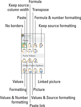
Figure 4-9: Clicking the Paste Options button or pressing the Ctrl key after completing a paste operation gives you this palette of paste options.

You can use these paste options to control or restrict the type of content and formatting that’s included in the pasted cell range. The paste options (complete with the hot key sequences you can type to select them) on the Paste Options palette include:

Paste (P): Excel pastes all the stuff in the cell selection (formulas, formatting, you name it).

Formulas (F): Excel pastes all the text, numbers, and formulas in the current cell selection without their formatting.

Formulas & Number Formatting (O): Excel pastes the number formats assigned to the copied values along with their formulas.

Keep Source Formatting (K): Excel copies the formatting from the original cells and pastes this into the destination cells (along with the copied entries).

No Borders (B): Excel pastes all the stuff in the cell selection without copying any borders applied to its cell range.

Keep Source Column Widths (W): Excel makes the width of the columns in the destination range the same as those in the source range when it copies their cell entries.

Transpose (T): Excel changes the orientation of the pasted entries. For example, if the original cells’ entries run down the rows of a single column of the worksheet, the transposed pasted entries will run across the columns of a single row.

Values (V): Excel pastes only the calculated results of any formulas in the source cell range.

Values & Number Formatting (A): Excel pastes the calculated results of any formulas along with all the formatting assigned to the labels, values, and formulas in the source cell range into the destination range. This means that all the labels and values in the destination range appear formatted just like the source range, even though all the original formulas are lost and only the calculated values are retained.

Values & Source Formatting (E): Excel pastes the calculated results of any formulas along with all formatting assigned to the source cell range.

Formatting (R): Excel pastes only the formatting (and not the entries) copied from the source cell range to the destination range.

Paste Link (N): Excel creates linking formulas in the destination range so that any changes that you make to the entries in cells in the source range are immediately brought forward and reflected in the corresponding cells of the destination range.

Picture (U): Excel pastes only the pictures in the copied cell selection.

Linked Picture (I): Excel pastes a link to the pictures in the copied cell selection.

The options that appear on the Paste Options palette are context sensitive. This means that the particular paste options available on the palette depend directly upon the type of cell entries previously copied to the Office Clipboard. Additionally, you can access this same palette of paste options by clicking the drop-down button that appears directly beneath the Paste button on the Ribbon instead of clicking the Paste Options button that appears at the end of the pasted range in the worksheet or pressing the Ctrl key on your keyboard.

Paste it from the Clipboard task pane

The Clipboard can store multiple cuts and copies from any program running under Windows (not just Excel). In Excel, this means that you can continue to paste stuff from the Clipboard into a workbook even after finishing a move or copy operation (even when you do so by pressing the Enter key rather than using the Paste command).

To open the Clipboard in its own task pane to the immediate left of the Worksheet area (see Figure 4-10), click the Dialog Box launcher in the lower-right corner of the Clipboard group on the Ribbon’s Home tab.

Figure 4-10: The Clipboard task pane appears on the left side of the Excel Worksheet area.

To paste an item from the Office Clipboard into a worksheet other than the one with the data last cut or copied onto it, click the item in the Clipboard task pane to paste it into the worksheet starting at the current position of the cell cursor.

You can paste all the items stored in the Office Clipboard into the current worksheet by clicking the Paste All button at the top of the Clipboard task pane. To clear the Office Clipboard of all the current items, click the Clear All button. To delete only a particular item from the Office Clipboard, position the mouse pointer over the item in the Clipboard task pane until its drop-down button appears. Click this drop-down button, and then choose Delete from the pop-up menu (refer to Figure 4-10).

To have the Clipboard task pane appear automatically after making two cuts or copies to the Clipboard in an Excel workbook, click the Show Office Clipboard Automatically option on the task pane’s Options button menu. To open the Clipboard task pane in the Excel program window by pressing Ctrl+CC, click Show Office Clipboard When Ctrl+C Pressed Twice on the task pane’s Options button. Pressing Ctrl+CC only opens the task pane. You still have to click the Close button on the Office Clipboard to close the task pane.

So what’s so special about Paste Special?

Normally, unless you fool around with the Paste Options (see the section “Keeping pace with Paste Options,” earlier in this chapter), Excel copies all the information in the range of cells you selected: formatting, as well the formulas, text, and other values you enter. You can use the Paste Special command to specify which entries and formatting to use in the current paste operation. Many of the Paste Special options are also available on the Paste Options palette.

To paste particular parts of a cell selection while discarding others, click the drop-down button that appears at the bottom of the Paste command button on the Ribbon’s Home tab. Then, click Paste Special on its drop-down menu to open the Paste Special dialog box, shown in Figure 4-11.

Figure 4-11: Use the options in the Paste Special dialog box to control what part of the copied cell selection to include in the paste operation.

The options in the Paste Special dialog box include:

All to paste all the stuff in the cell selection (formulas, formatting, you name it).

Formulas to paste all the text, numbers, and formulas in the current cell selection without their formatting.

Values to convert formulas in the current cell selection to their calculated values.

Formats to paste only the formatting from the current cell selection, leaving the cell entries in the dust.

Comments to paste only the notes that you attach to their cells (kind of like electronic self-stick notes — see Chapter 6 for details).

Validation to paste only the data validation rules into the cell range that you set up with the Data Validation command (which enables you to set what value or range of values is allowed in a particular cell or cell range).

All Using Source Theme to paste all the information plus the cell styles applied to the cells.

All Except Borders to paste all the stuff in the cell selection without copying any borders you use there.

Column Widths to apply the column widths of the cells copied to the Clipboard to the columns where the cells are pasted.

Formulas and Number Formats to include the number formats assigned to the pasted values and formulas.

Values and Number Formats to convert formulas to their calculated values and include the number formats you assign to all the pasted values.

All Merging Conditional Formats to paste Conditional Formatting into the cell range.

None to prevent Excel from performing any mathematical operation between the data entries you cut or copy to the Clipboard and the data entries in the cell range where you paste.

Add to add the data you cut or copy to the Clipboard and the data entries in the cell range where you paste.

Subtract to subtract the data you cut or copy to the Clipboard from the data entries in the cell range where you paste.

Multiply to multiply the data you cut or copy to the Clipboard by the data entries in the cell range where you paste.

Divide to divide the data you cut or copy to the Clipboard by the data entries in the cell range where you paste.

Skip Blanks check box when you want Excel to paste everywhere except for any empty cells in the incoming range. In other words, a blank cell cannot overwrite your current cell entries.

Transpose check box when you want Excel to change the orientation of the pasted entries. For example, if the original cells’ entries run down the rows of a single column of the worksheet, the transposed pasted entries will run across the columns of a single row.

Paste Link button when you’re copying cell entries and you want to establish a link between copies you’re pasting and the original entries. That way, changes to the original cells automatically update in the pasted copies.

Let’s Be Clear about Deleting Stuff

No discussion about editing in Excel would be complete without a section on getting rid of the stuff you put into cells. You can perform two kinds of deletions in a worksheet:

Clearing a cell: Clearing just deletes or empties the cell’s contents without removing the cell from the worksheet, which would alter the layout of the surrounding cells.

Deleting a cell: Deleting gets rid of the whole kit and caboodle — cell structure along with all its contents and formatting. When you delete a cell, Excel has to shuffle the position of entries in the surrounding cells to plug up any gaps made by the action.

Sounding the all clear!

To get rid of just the contents of a cell selection rather than delete the cells and their contents, select the range of cells to clear and then simply press the Delete key.

If you want to get rid of more than just the contents of a cell selection, click the Clear button (the one with the eraser) in the Editing group on the Ribbon’s Home tab and then click one of the following options on its drop-down menu:

Clear All: Gets rid of all formatting and notes, as well as entries in the cell selection (Alt+HEA).

Clear Formats: Deletes only the formatting from the cell selection without touching anything else (Alt+HEF).

Clear Contents: Deletes only the entries in the cell selection just like pressing the Delete key (Alt+HEC).

Clear Comments: Removes the notes in the cell selection but leaves everything else behind (Alt+HEM).

Clear Hyperlinks: Removes the active hyperlinks (see Chapter 12) in the cell selection but leaves its descriptive text (Alt+HEL).

Remove Hyperlinks: Removes the active hyperlinks in the cell selection along with all the formatting (Alt+HER).

Get these cells outta here!

To delete the cell selection rather than just clear out its contents, select the cell range, click the drop-down button attached to the Delete command button in the Cells group of the Home tab, and then click Delete Cells on the drop-down menu (or press Alt+HDD). The Delete dialog box opens, showing options for filling in the gaps created when the cells currently selected are blotted out of existence:

Shift Cells Left: This default option moves entries from neighboring columns on the right to the left to fill in gaps created when you delete the cell selection by clicking OK or pressing Enter.

Shift Cells Up: Select this to move entries up from neighboring rows below.

Entire Row: Select this to remove all the rows in the current cell selection.

Entire Columns: Select this to delete all the columns in the current cell selection.

If you know that you want to shift the remaining cells to the left after deleting the cells in the current selection, you can simply click the Delete command button on the Home tab of the Ribbon. (This is the same thing as opening the Delete dialog box and then clicking OK when the default Shift Cells Left button is selected.

To delete an entire column or row from the worksheet, you can select the column or row on the workbook window frame, right-click the selection, and then click Delete from the column’s or row’s shortcut menu.

You can also delete entire columns and rows selected in the worksheet by clicking the drop-down button attached to the Delete command button on the Ribbon’s Home tab and then clicking the Delete Sheet Columns (Alt+HDC) option or the Delete Sheet Rows option (Alt+HDR) on the drop-down menu.

Deleting entire columns and rows from a worksheet is risky business unless you are sure that the columns and rows in question contain nothing of value. Remember, when you delete an entire row from the worksheet, you delete all information from column A through XFD in that row (and you can see only a very few columns in this row). Likewise, when you delete an entire column from the worksheet, you delete all information from row 1 through 1,048,576 in that column.

Staying in Step with Insert

For those inevitable times when you need to squeeze new entries into an already populated region of the worksheet, you can insert new cells in the area rather than go through all the trouble of moving and rearranging several individual cell ranges. To insert a new cell range, select the cells (many of which are already occupied) where you want the new cells to appear and then click the drop-down button on the right end of the Insert command button (rather than the button itself) in the Cells group of the Home tab and then click Insert Cells on the drop-down menu (or press Alt+HII). The Insert dialog box opens with the following option buttons:

Shift Cells Right: Select this to shift existing cells to the right to make room for the ones you want to add before clicking OK or pressing Enter.

Shift Cells Down: Use this default to instruct the program to shift existing entries down before clicking OK or pressing Enter.

Entire Row or Entire Column: When you insert cells with the Insert dialog box, you can insert complete rows or columns in the cell range by selecting either of these radio buttons. You can also select the row number or column letter on the frame before you choose the Insert command.

If you know that you want to shift the existing cells to the right to make room for the newly inserted cells, you can simply click the Insert command button on the Ribbon’s Home tab (this is the same thing as opening the Insert dialog box and then clicking OK when the Shift Cells Right button is selected).

Remember that you can also insert entire columns and rows in a worksheet by right-clicking the selection and then clicking Insert on the column’s or row’s shortcut menu.

As when you delete whole columns and rows, inserting entire columns and rows affects the entire worksheet, not just the part you see. If you don’t know what’s out in the hinterlands of the worksheet, you can’t be sure how the insertion will affect — perhaps even sabotage — stuff (especially formulas) in the other unseen areas. I suggest that you scroll all the way out in both directions to make sure that nothing’s out there.

Stamping Out Your Spelling Errors

If you’re as good a speller as I am, you’ll be relieved to know that Excel 2013 has a built-in spell checker that can catch and remove all those embarrassing little spelling errors. With this in mind, you no longer have any excuse for putting out worksheets with typos in the titles or headings.

To check the spelling in a worksheet, you have the following options:

Click the Spelling command button on the Ribbon’s Review tab

Press Alt+RS

Press F7

Any way you do it, Excel begins checking the spelling of all text entries in the worksheet. When the program comes across an unknown word, it displays the Spelling dialog box, similar to the one shown in Figure 4-12.

Figure 4-12: Check your spelling from the Spelling dialog box.

Excel suggests replacements for the unknown word shown in the Not in Dictionary text box with a likely replacement in the Suggestions list box of the Spelling dialog box. If that replacement is incorrect, you can scroll through the Suggestions list and click the correct replacement. Use the Spelling dialog box options as follows:

Ignore Once and Ignore All: When Excel’s spell check comes across a word its dictionary finds suspicious but you know is viable, click the Ignore Once button. If you don’t want the spell checker to bother querying you about this word again, click the Ignore All button.

Add to Dictionary: Click this button to add the unknown (to Excel) word — such as your name — to a custom dictionary so that Excel won’t flag it again when you check the spelling in the worksheet later on.

Change: Click this button to replace the word listed in the Not in Dictionary text box with the word Excel offers in the Suggestions list box.

Change All: Click this button to change all occurrences of this misspelled word in the worksheet to the word Excel displays in the Suggestions list box.

AutoCorrect: Click this button to have Excel automatically correct this spelling error with the suggestion displayed in the Suggestions list box (by adding the misspelling and suggestion to the AutoCorrect dialog box; for more, read Chapter 2).

Dictionary Language: To switch to another dictionary (such as a United Kingdom English dictionary, or a French dictionary when checking French terms in a multilingual worksheet), click this drop-down button and then select the name of the desired language in the list.

Options button to open the Proofing tab in the Excel Options dialog box where you can modify the current Excel spell-check settings such as Ignore Words in Uppercase, Ignore Words with Numbers, and the like.

Notice that the Excel spell checker not only flags words not found in its built-in or custom dictionary, but also flags occurrences of double words in a cell entry (such as total total) and words with unusual capitalization (such as NEw York instead of New York). By default, the spell checker ignores all words with numbers and all Internet addresses. If you want it to ignore all words in uppercase letters as well, click the Options button at the bottom of the Spelling dialog box, and then select the Ignore Words in UPPERCASE check box before clicking OK.

You can check the spelling of just a particular group of entries by selecting the cells before you click the Spelling command button on the Review tab of the Ribbon or press F7.

Excel also has a Thesaurus pane that enables you to find synonyms for the label entered into the cell that’s current when you open the pane (or that you type into its text box). To open the Thesaurus pane, select Review⇒Thesaurus in the Proofing group at the beginning of the Review tab on the Ribbon or press Shift+F7. Excel then opens a pane showing a list of all the synonyms for the label in the current cell or the term manually entered in its text box. To view more synonyms for a particular term in the list, select it. To replace the label entered in the current cell with a term in the Thesaurus list, select Insert on the term’s drop-down menu.

Eliminating Errors with Text to Speech

The good news is that Excel 2013 still supports the Text to Speech feature introduced in Excel 2003. This feature enables your computer to read aloud any series of cell entries in the worksheet. By using Text to Speech, you can check your printed source while the computer reads aloud the values and labels that you’ve actually entered — a real nifty way to catch and correct errors that may otherwise escape unnoticed.

The Text to Speech translation feature requires no prior training or special microphones: All that’s required is a pair of speakers or headphones connected to your computer.

Now for the bad news: Text to Speech is not available from any of the tabs on the Ribbon. The only way to access Text to Speech is by adding its Speak Cells command buttons as custom buttons on the Quick Access toolbar to a custom tab on the Ribbon.

Here are the steps for adding the Text to Speech command buttons to the Quick Access toolbar (shown in Figure 4-13):

1. Click Customize Quick Access Toolbar button at the end of the toolbar followed by the More Commands on the Customize Quick Access toolbar on its drop-down menu.

The Excel Options dialog box opens with the Customize Access Toolbar tab selected.

2. Click Commands Not in the Ribbon on the Choose Commands From drop-down menu and scroll down the list until you see the Speak Cells command.

The Text to Speech command buttons include Speak Cells, Speak Cells – Stop Speaking Cells, Speak Cells by Columns, Speak Cells by Rows, and Speak Cells on Enter.

3. Click the Speak Cells button in the Choose Commands From list box on the left and then click the Add button to add it to the Quick Access toolbar following the Redo button.

4. Click the Add button repeatedly until you’ve added the remaining Text to Speech buttons to the custom group: Speak Cells – Stop Speaking Cells, Speak Cells by Columns, Speak Cells by Rows, and Speak Cells on Enter.

To reposition the speech command buttons on the Quick Access toolbar, select the button and then move it up or down in the list (which corresponds to left and right, respectively on the toolbar) with the Move Up and Move Down.

5. Click the OK button to close the Excel Options dialog box.

Figure 4-13 shows the Quick Access toolbar above my Ribbon in my Excel 2013 program window after I added the speech buttons to it.

Figure 4-13: After adding the Speak Cells buttons to Quick Access toolbar, you can use them to check cell entries audibly.

After adding the Text to Speech commands as custom Speak Cells buttons to your Quick Access toolbar, you can use them to corroborate spreadsheet entries and catch those hard-to-spot errors as follows:

1. Select the cells in the worksheet whose contents you want read aloud by Text to Speech.

2. Click the Speak Cells button on the Quick Access toolbar to have the computer read the entries in the selected cells.

By default, the Text to Speech feature reads the contents of each cell in the cell selection by reading down each column and then across the rows. If you want Text to Speech to read across the rows and then down the columns, click the Speak Cells by Rows button on the Quick Access toolbar (the button with the two opposing horizontal arrows).

3. To have the Text to Speech feature read each cell entry while you press the Enter key (at which point the cell cursor moves down to the next cell in the selection), click the Speak Cells on Enter custom button (the button with the curved arrow Enter symbol) on your Quick Access toolbar.

As soon as you click the Speak Cells on Enter button, the computer tells you, “Cells will now be spoken on Enter.” After selecting this option, you need to press Enter each time that you want to hear an entry read to you.

4. To pause the Text to Speech feature when you’re not using the Speak Cells on Enter option (Step 3) and you locate a discrepancy between what you’re reading and what you’re hearing, click the Stop Speaking button (the Speak Cells group button with the x).

After you click the Speak Cells on Enter button on the Quick Access toolbar, the Text to Speech feature speaks aloud each new cell entry you make after you complete it by pressing any of the keys — Enter, Tab, Shift+Tab, one of the arrow keys, and so forth — that move the cell pointer upon making the cell entry. Text to Speech does not, however, speak a cell entry that you complete by clicking the Enter button on the Formula bar because this action does not move the cell pointer upon completing the cell entry.