
Chapter 6
Maintaining the Worksheet
In This Chapter
![]() Zooming in and out on a worksheet
Zooming in and out on a worksheet
![]() Splitting the workbook window into two or four panes
Splitting the workbook window into two or four panes
![]() Freezing columns and rows onscreen for worksheet titles
Freezing columns and rows onscreen for worksheet titles
![]() Attaching comments to cells
Attaching comments to cells
![]() Naming your cells
Naming your cells
![]() Finding and replacing stuff in your worksheet
Finding and replacing stuff in your worksheet
![]() Looking up stuff using online resources in the Research task pane
Looking up stuff using online resources in the Research task pane
![]() Controlling when you recalculate a worksheet
Controlling when you recalculate a worksheet
![]() Protecting your worksheets
Protecting your worksheets
Each worksheet in an Excel 2013 workbook offers an immense place in which to store information. But because even a regular size computer monitor (which is quite large when compared to a Windows tablet or smartphone screen) lets you see only a tiny bit of any of the worksheets in a workbook at a time, the issue of keeping on top of information is not a small one (pun intended).
Although the Excel worksheet employs a coherent cell-coordinate system that you can use to get anywhere in the great big worksheet, you have to admit that this A1, B2 stuff — although highly logical — remains fairly alien to human thinking. (I mean, saying, “Go to cell IV88,” just doesn’t have anywhere near the same impact as saying, “Go to the corner of Hollywood and Vine.”) Consider for a moment the difficulty of coming up with a meaningful association between the 2008 depreciation schedule and its location in the cell range AC50:AN75 so that you can remember where to find it.
In this chapter, I show you some of the more effective techniques for maintaining and keeping on top of information. You find out how to change the perspective on a worksheet by zooming in and out on the information, how to split the document window into separate panes so that you can display different sections of the worksheet at the same time, and how to keep particular rows and columns on the screen at all times.
And, as if that weren’t enough, you also see how to add comments to cells, assign descriptive, English-type names to cell ranges (like Hollywood_and_Vine!), and use the Find and Replace commands to locate and, if necessary, replace entries anywhere in the worksheet. Finally, you see how to control when Excel recalculates the worksheet and how to limit where changes can be made.
Zooming In and Out
So what to do when trying to edit the company’s huge spreadsheet on your fancy new Microsoft Surface Pro tablet with its not-so-generous 10.6-inch screen or even on your 14-inch screen laptop? Does this mean that you’re doomed to straining your eyes to read all the information in those tiny cells, or you’re scrolling like mad trying to locate a table you can’t seem to find? Never fear, the Zoom feature is here in the form of the Zoom slider on the Status bar. You can use the Zoom slider to quickly increase the magnification of part of the worksheet or shrink it down to the tiniest size.
You can use the Zoom slider on the Status bar of the Excel window in several ways, depending upon the device you’re using:
![]() Drag the Zoom slider button to the left or the right on the slider to decrease or increase the magnification percentage (with 10% magnification being the lowest percentage when you drag all the way to the left on the slider and 400% magnification being the highest percentage when you drag all the way to the right).
Drag the Zoom slider button to the left or the right on the slider to decrease or increase the magnification percentage (with 10% magnification being the lowest percentage when you drag all the way to the left on the slider and 400% magnification being the highest percentage when you drag all the way to the right).
![]() Click the Zoom Out (with the minus sign) or the Zoom In button (with the plus sign) at either end of the slider to decrease or increase the magnification percentage by 10%.
Click the Zoom Out (with the minus sign) or the Zoom In button (with the plus sign) at either end of the slider to decrease or increase the magnification percentage by 10%.
![]() Use the stretch-and-pinch gesture with your thumb and forefinger on your touchscreen device to quickly zoom in and out on the cells of your worksheet and move the Zoom slider at the same time.
Use the stretch-and-pinch gesture with your thumb and forefinger on your touchscreen device to quickly zoom in and out on the cells of your worksheet and move the Zoom slider at the same time.
In Figure 6-1, you can see a blowup of the worksheet after increasing it to 200% magnification (twice the normal size). To blow up a worksheet like this, drag the Zoom slider button to the right until 200% appears on the Status bar to the left of the slider. (You can also do this by clicking View⇒Zoom and then clicking the 200% button in the Zoom dialog box, if you really want to go to all that trouble.) One thing’s for sure: You don’t have to go after your glasses to read the names in those enlarged cells! The only problem with 200% magnification is that you can see only a few cells at one time.
In Figure 6-2, check out the same worksheet, this time at 40%magnification. To reduce the display to this magnification, you drag the Zoom slider button to the left until 40% appears on the Status bar in front of the slider.
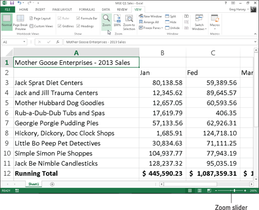
Figure 6-1: Zooming a sample worksheet to 200% magnification.
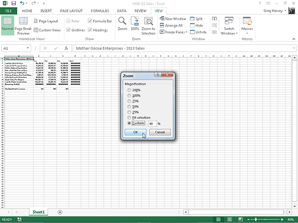
Figure 6-2: Zooming a sample worksheet to 40% magnification.
Whew! At 40% of normal screen size, the only thing you can be sure of is that you can’t read a thing! However, notice that with this bird’s-eye view, you can see at a glance how far over and down the data in this worksheet extends and how much empty space there is in the worksheet.
The Zoom dialog box (View⇒Zoom or Alt+WQ) offers five precise magnification settings — 200%, 100% (normal screen magnification), 75%, 50%, and 25%. To use other percentages besides those, you have the following options:
![]() If you want to use precise percentages other than the five preset percentages (such as 150% or 85%) or settings greater or less than the highest or lowest percentage (such as 400% or 10%), click within the Custom button’s text box in the Zoom dialog box, type the new percentage, and press Enter.
If you want to use precise percentages other than the five preset percentages (such as 150% or 85%) or settings greater or less than the highest or lowest percentage (such as 400% or 10%), click within the Custom button’s text box in the Zoom dialog box, type the new percentage, and press Enter.
![]() If you don’t know what percentage to enter in order to display a particular cell range on the screen, select the range, click View⇒Zoom to Selection on the Ribbon or press Alt+WG. Excel figures out the percentage necessary to fill your screen with just the selected cell range.
If you don’t know what percentage to enter in order to display a particular cell range on the screen, select the range, click View⇒Zoom to Selection on the Ribbon or press Alt+WG. Excel figures out the percentage necessary to fill your screen with just the selected cell range.
 To quickly return to 100% (normal) magnification in the worksheet after selecting any another percentage, all you have to do is click the bar in the center of the Zoom slider on the Status bar or click the 100% button on the View tab of the Ribbon.
 You can use the Zoom feature to locate and move to a new cell range in the worksheet. First, select a small magnification, such as 50%. Then locate the cell range you want to move to and select one of its cells. Finally, use the Zoom feature to return the screen magnification to 100%. When Excel returns the display to normal size, the cell you select and its surrounding range appear onscreen.
Splitting the Worksheet into Windows
Although zooming in and out on the worksheet can help you get your bearings, it can’t bring together two separate sections so that you can compare their data on the screen (at least not at a normal size where you can actually read the information). To manage this kind of trick, split the Worksheet area into separate panes and then scroll the worksheet in each pane so that they display the parts you want to compare.
Splitting the window is easy. Look at Figure 6-3 to see an Income Analysis worksheet after splitting its worksheet window horizontally into two panes and scrolling up rows 38 through 44 in the lower pane. Each pane has its own vertical scroll bar, which enables you to scroll different parts of the worksheet into view.
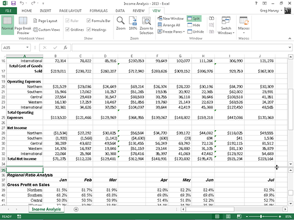
Figure 6-3: The Income Analysis spreadsheet in a split window after scrolling up the bottom rows in the lower pane.
To split a worksheet into two (upper and lower) horizontal panes, you simply position the cell pointer at the place in the worksheet where you want to split the worksheet and then click the Split button on the Ribbon’s View tab (or press Alt+WS).
The key to the panes created with the Split button is the cell in the worksheet where you position the pointer before selecting this command button:
![]() To split the window into two horizontal panes, position the cell pointer in column A of the row where you want to split the worksheet
To split the window into two horizontal panes, position the cell pointer in column A of the row where you want to split the worksheet
![]() To split the window into two vertical panes, position the cell pointer in row 1 of the column where you want to split the worksheet
To split the window into two vertical panes, position the cell pointer in row 1 of the column where you want to split the worksheet
![]() To split the window into four panes — two horizontal and two vertical — position the cell pointer along the top and left edge of cell.
To split the window into four panes — two horizontal and two vertical — position the cell pointer along the top and left edge of cell.
After you split the worksheet window, Excel displays a split bar (a thin, light gray bar) along the row or column where the window split occurs. If you position the mouse or touch pointer anywhere on the split bar, the pointer changes from a white-cross to a split pointer shape (with black arrowheads pointing in opposite directions from parallel separated lines).
You can increase or decrease the size of the current window panes by dragging the split bar up or down or left or right with the split pointer. You can make the panes in a workbook window disappear by double-clicking anywhere on the split bar (you can also do this by selecting View⇒Split again).
Fixed Headings with Freeze Panes
Panes are great for viewing different parts of the same worksheet that normally can’t be seen together. You can also use panes to freeze headings in the top rows and first columns so that the headings stay in view at all times, no matter how you scroll through the worksheet. Frozen headings are especially helpful when you work with a table that contains information that extends beyond the rows and columns shown onscreen.
In Figure 6-4, you can see just such a table. The Income Analysis worksheet contains more rows and columns than you can see at one time (unless you decrease the magnification to about 40% with Zoom, which makes the data too small to read). In fact, this worksheet continues down to row 52 and over to column P.
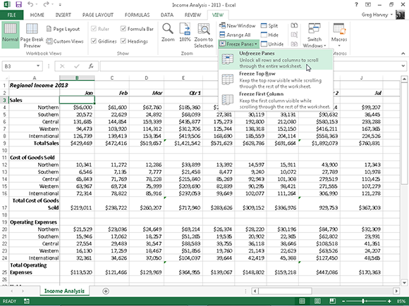
Figure 6-4: Frozen panes keep the column headings and the row headings on the screen at all times.
By dividing the worksheet into four panes between rows 2 and 3 and columns A and B and then freezing them on the screen, you can keep the column headings in row 2 that identify each column of information on the screen while you scroll the worksheet up and down to review information on income and expenses. Additionally, you can keep the row headings in column A on the screen while you scroll the worksheet to the right.
Refer to Figure 6-4 to see the worksheet right after splitting the window into four panes and freezing them. To create and freeze these panes, follow these steps:
1. Position the cell cursor in cell B3.
2. Click View⇒Freeze Panes on the Ribbon and then click Freeze Panes on the drop-down menu or press Alt+WFF.
In this example, Excel freezes the top and left pane above row 3 and left of column B.
When Excel sets up the frozen panes, the borders of frozen panes are represented by a single line rather than the thin gray bar, as is the case when simply splitting the worksheet into panes.
See what happens when you scroll the worksheet up after freezing the panes (shown in Figure 6-5). In this figure, I scrolled the worksheet up so that rows 33 through 52 of the table appear under rows 1 and 2. Because the vertical pane with the worksheet title and column headings is frozen, it remains onscreen. (Normally, rows 1 and 2 would have been the first to disappear when you scroll the worksheet up.)
Look to Figure 6-6 to see what happens when you scroll the worksheet to the right. In this figure, I scroll the worksheet so that the data in columns M through P appear after the data in column A. Because the first column is frozen, it remains onscreen, helping you identify the various categories of income and expenses for each month.
Click Freeze Top Row or Freeze First Column on the Freeze Panes button’s drop-down menu to freeze the column headings in the top row of the worksheet or the row headings in the first column of the worksheet, regardless of where the cell cursor is located in the worksheet.
To unfreeze the panes in a worksheet, click View⇒Freeze Panes on the Ribbon and then click Unfreeze Panes on the Freeze Panes button’s drop-down menu or press Alt+WFF. Choosing this option removes the panes, indicating that Excel has unfrozen them.
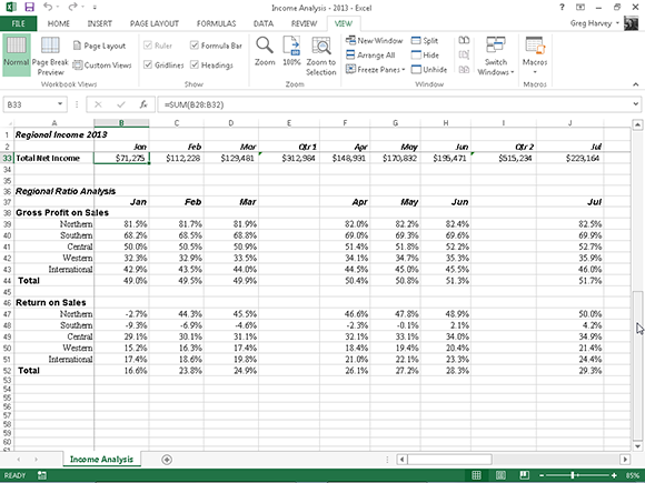
Figure 6-5: The Income Analysis worksheet after scrolling the rows up to display additional income and expense data.

Figure 6-6: The Income Analysis worksheet after scrolling the columns left to display the last group of columns in this table.
Electronic Sticky Notes
You can add text comments to particular cells in an Excel worksheet. Comments act kind of like electronic pop-up versions of sticky notes. For example, you can add a comment to yourself to verify a particular figure before printing the worksheet or to remind yourself that a particular value is only an estimate (or even to remind yourself that it’s your anniversary and to pick up a little something special for your spouse on the way home!).
In addition to using notes to remind yourself of something you’ve done or that remains to be done, you can also use a comment to mark your current place in a large worksheet. You can then use the comment’s location to quickly find your starting place the next time you work with that worksheet.
Adding a comment to a cell
To add a comment to a cell, follow these steps:
1. Move the cell pointer to or click the cell to which you want to add the comment.
2. Click the New Comment command button on the Ribbon’s Review tab or press Alt+RC.
A new text box appears (similar to the one shown in Figure 6-7). This text box contains the name of the user as it appears in the User Name text box on the General tab in the Excel Options dialog box (Alt+FT) and the insertion point located at the beginning of a new line right below the user name.
3. Type the text of your comment in the text box that appears.
4. When you finish entering the comment text, click somewhere on the worksheet outside of the text box.
Excel marks the location of a comment in a cell by adding a tiny triangle in the upper-right corner of the cell. (This triangular indicator appears in red on a color monitor.)
5. To display the comment in a cell, position the thick white cross mouse or touch pointer somewhere in the cell with the note indicator.

Figure 6-7: Adding a comment to a cell in a new text box.
Comments in review
When you have a workbook with sheets that contain a bunch of comments, you probably won’t want to take the time to position the mouse pointer over each of its cells in order to read each one. For those times, you need to click the Show All Comments command button on the Ribbon’s Review tab (or press Alt+RA). When you click Show All Comments on the Review tab, Excels displays all the comments in the workbook (as shown in Figure 6-8).
With the Review tab selected in the Ribbon, you can then move back and forth from comment to comment by clicking its Next and Previous command buttons in the Comments group (or by pressing Alt+RN and Alt+RV, respectively). When you reach the last comment in the workbook, you receive an alert box asking you whether you want to continue reviewing the comments from the beginning (which you can do by simply clicking OK). After you finish reviewing the comments in your workbook, you can hide their display by clicking the Show All Comments command button on the Review tab of the Ribbon or pressing Alt+RA a second time.
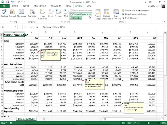
Figure 6-8: Use the Show All Comments button on the Review tab to review the comments added to a worksheet.
Editing comments in a worksheet
To edit the contents of a comment, select it by clicking the Next or Previous command button in the Comments group of the Review tab and then click the Edit Comment button (which replaces New Comment) or right-click the cell with the comment and select Edit Comment from the cell’s shortcut menu. You can also do this by selecting the cell with the comment and then pressing Shift+F2.
To change the placement of a comment in relation to its cell, you select the comment by clicking somewhere on it and then position the mouse pointer on one of the edges of its text box. When a four-headed arrow appears at the tip of the mouse or touch pointer, you can drag the text box to a new place in the worksheet. When you release the mouse button, finger, or stylus, Excel redraws the arrow connecting the comment’s text box to the note indicator in the upper-right corner of the cell.
To change the size of a comment’s text box, you select the comment, position the mouse or touch pointer on one of its sizing handles, and then drag in the appropriate direction (away from the center of the box to increase its size or toward the center to decrease its size). When you release the mouse button finger, or stylus, Excel redraws the comment’s text box with the new shape and size. When you change the size and shape of a comment’s text box, Excel automatically wraps the text to fit in the new shape and size.
To change the font of the comment text, select the text of the comment (by selecting the comment for editing and then dragging through the text), right-click the text box, and then click Format Comment on its shortcut menu (or you can press Ctrl+1 as I do). On the Font tab of the Format Cells dialog box that appears, you can then use the options to change the font, font style, font size, or color of the text displayed in the selected comment.
To delete a comment, select the cell with the comment in the worksheet or click the Next or Previous command buttons on the Review tab of the Ribbon until the comment is selected and then click the Delete command button in the Comments group (Alt+RD). Excel removes the comment along with the note indicator from the selected cell.
You can also delete all comments in the selected range by clicking Clear Comments from the Clear button’s drop-down menu (the one with the eraser icon in the Editing group) on the Home tab of the Ribbon (Alt+HEM).
Getting your comments in print
When printing a worksheet, you can print comments along with worksheet data by selecting either At End of Sheet or As Displayed on Sheet on the Comments drop-down list on the Sheet tab of the Page Setup dialog box. Open this dialog box by clicking the Dialog Box launcher in the lower-right corner of the Page Setup group on the Ribbon’s Page Layout tab (Alt+PSP).
The Range Name Game
By assigning descriptive names to cells and cell ranges, you can go a long way toward keeping on top of the location of important information in a worksheet. Rather than try to associate random cell coordinates with specific information, you just have to remember a name. You can also use range names to designate the cell selection that you want to print or use in other Office 2013 programs, such as Microsoft Word or Access. Best of all, after you name a cell or cell range, you can use this name with the Go To feature to not only locate the range but select all its cells as well.
 I’ve always been a fan of using range names in worksheets for all the previous versions of Excel designed for desktop and laptop computers. With this new version of Excel designed for touchscreen devices, such as Windows 8 tablets and smartphones, as well, I’m bordering on becoming a fanatic about their use. Believe me, you can save yourself oodles of time save and tons of frustration by locating and a selecting the data tables and lists in your worksheets on these touch devices via range names. Contrast simply tapping their range names on Excel’s Name box’s drop-down list to go to and select them to having first to swipe and swipe to locate and display their cells before dragging through their cells with your finger or stylus.
If I only had a name . . .
When assigning range names to a cell or cell range, you need to follow a few guidelines:
![]() Range names must begin with a letter of the alphabet, not a number.
Range names must begin with a letter of the alphabet, not a number.
For example, instead of 01Profit, use Profit01.
![]() Range names cannot contain spaces.
Range names cannot contain spaces.
Instead of a space, use the underscore (Shift+hyphen) to tie the parts of the name together. For example, instead of Profit 01, use Profit_01.
![]() Range names cannot correspond to cell coordinates in the worksheet.
Range names cannot correspond to cell coordinates in the worksheet.
For example, you can’t name a cell Q1 because this is a valid cell coordinate. Instead, use something like Q1_sales.
To name a cell or cell range in a worksheet, follow these steps:
1. Select the cell or cell range that you want to name.
2. Click the cell address for the current cell that appears in the Name Box on the far left of the Formula bar.
Excel selects the cell address in the Name Box.
3. Type the name for the selected cell or cell range in the Name Box.
When typing the range name, you must follow Excel’s naming conventions: Refer to the bulleted list of cell-name do’s and don’ts earlier in this section for details.
4. Press Enter.
To select a named cell or range in a worksheet, click the range name on the Name Box drop-down list. To open this list, click the drop-down arrow button that appears to the right of the cell address on the Formula bar.
You can also accomplish the same thing by selecting Home⇒Find & Select⇒Go To or by pressing F5 or Ctrl+G to open the Go To dialog box (see Figure 6-9). Double-click the desired range name in the Go To list box (alternatively, select the name followed by OK). Excel moves the cell cursor directly to the named cell. If you select a cell range, all the cells in that range are selected as well.
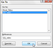
Figure 6-9: Select the named cell range to go to in a workbook.
Name that formula!
Cell names are not only a great way to identify and find cells and cell ranges in your spreadsheet, but they’re also a great way to make out the purpose of your formulas. For example, suppose that you have a simple formula in cell K3 that calculates the total due to you by multiplying the hours you work for a client (in cell I3) by the client’s hourly rate (in cell J3). Normally, you would enter this formula in cell K3 as
=I3*J3
However, if you assign the name Hours to cell I3 and the name Rate to cell J3, in cell K3 you could enter the formula
=Hours*Rate
I don’t think there’s anyone who would dispute that the formula =Hours*Rate is much easier to understand than =I3*J3.
To enter a formula using cell names rather than cell references, follow these steps (see Chapter 2 to brush up on how to create formulas):
1. Assign range names to the individual cells as I describe earlier in this section.
For this example, give the name Hours to cell I3 and the name Rate to cell J3.
2. Place the cell cursor in the cell where the formula is to appear.
For this example, put the cell cursor in cell K3.
3. Type = (equal sign) to start the formula.
4. Select the first cell referenced in the formula by selecting its cell (either by clicking the cell or moving the cell cursor into it).
For this example, you select the Hours cell by selecting cell I3.
5. Type the arithmetic operator to use in the formula.
For this example, you would type * (asterisk) for multiplication. (Refer to Chapter 2 for a list of the other arithmetic operators.)
6. Select the second cell referenced in the formula by selecting its cell (either by clicking the cell or moving the cell cursor into it).
For this example, you select the Rate cell by selecting cell J3.
7. Click the Enter button or press Enter to complete the formula.
In this example, Excel enters the formula =Hours*Rate in cell K3.
 You can’t use the fill handle to copy a formula that uses cell names, rather than cell addresses, to other cells in a column or row that perform the same function (see Chapter 4). When you copy an original formula that uses names rather than addresses, Excel copies the original formula without adjusting the cell references to the new rows and columns. See the upcoming “Naming constants” section to find a way to use your column and row headings to identify the cell references in the copies, and include the original formula from which the copies are made.
Naming constants
Certain formulas use constant values, such as an 8.25% tax rate or a 10% discount rate. If you don’t want to have to enter these constants into a cell of the worksheet in order to use the formulas, you create range names that hold their values and then use their range names in the formulas you create.
For example, to create a constant called tax_rate (of 8.25%), follow these steps:
1. Click the Define Name button on the Ribbon’s Formulas tab or press Alt+MMD to open the New Name dialog box.
2. In the New Name dialog box, type the range name (tax_rate in this example) into the Name text box.
Be sure to adhere to the cell range naming conventions when entering this new name.
3. (Optional) To have the range name defined for just the active worksheet instead of the entire workbook, click the name of the sheet on the Scope drop-down list.
Normally, you’re safer sticking with the default selection of Workbook as the Scope option so that you can use your constant in a formula on any of its sheets. Only change the scope to a particular worksheet when you’re sure that you’ll use it only in formulas on that worksheet.
4. Click in the Refers To text box after the equal to sign (=) and replace (enter) the current cell address with the constant value (8.25% in this example) or a formula that calculates the constant.
5. Click OK to close the New Name dialog box.
After you assign a constant to a range name by using this method, you can apply it to the formulas that you create in the worksheet in one of two ways:
![]() Type the range name to which you assign the constant at the place in the formula where its value is required.
Type the range name to which you assign the constant at the place in the formula where its value is required.
![]() Click the Use in Formula command button on the Formulas tab (or press Alt+MS) and then click the constant’s range name on the drop-down menu that appears.
Click the Use in Formula command button on the Formulas tab (or press Alt+MS) and then click the constant’s range name on the drop-down menu that appears.
When you copy a formula that uses a range name containing a constant, its values remain unchanged in all copies of the formula that you create with the fill handle. (In other words, range names in formulas act like absolute cell addresses in copied formulas — see Chapter 4 for more on copying formulas.)
Also, when you update the constant by changing its value in the Edit Name dialog box — opened by clicking the range name in the Name Manager dialog box (Alt+MN) and then clicking its Edit button — all the formulas that use that constant (by referring to the range name) are automatically updated (recalculated) to reflect this change.
Seek and Ye Shall Find . . .
When all else fails, you can use Excel’s Find feature to locate specific information in the worksheet. Choose Home⇒Find & Select⇒Find or press Ctrl+F, Shift+F5, or even Alt+HFDF to open the Find and Replace dialog box.
In the Find What drop-down box of this dialog box, enter the text or values you want to locate and then click the Find Next button or press Enter to start the search. Choose the Options button in the Find and Replace dialog box to expand the search options (as shown in Figure 6-10).
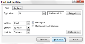
Figure 6-10: Use options in the Find and Replace dialog box to locate cell entries.
When you search for a text entry with the Find and Replace feature, be mindful of whether the text or number you enter in the Find What text box is separate in its cell or occurs as part of another word or value. For example, if you enter the characters in in the Find What text box and you don’t select the Match Entire Cell Contents check box, Excel finds
![]() The In in Regional Income 2010 in cell A1
The In in Regional Income 2010 in cell A1
![]() The In in International in A8, A16, A24 and so on
The In in International in A8, A16, A24 and so on
![]() The in in Total Operating Expenses in cell A25
The in in Total Operating Expenses in cell A25
If you select the Match Entire Cell Contents check box in the Find and Replace dialog box before starting the search, Excel would not consider the anything in the sheet to be a match because all entries have other text surrounding the text you’re searching for. If you had the state abbreviation for Indiana (IN) in a cell by itself and had chosen the Match Entire Cell Contents option, Excel would find that cell.
When you search for text, you can also specify whether you want Excel to match the case you use (uppercase or lowercase) when entering the search text in the Find What text box. By default, Excel ignores case differences between text in cells of your worksheet and the search text you enter in the Find What text box. To conduct a case-sensitive search, you need to select the Match Case check box (available when you click the Options button to expand the Find and Replace dialog box, shown in Figure 6-10).
If the text or values that you want to locate in the worksheet have special formatting, you can specify the formatting to match when conducting the search.
To have Excel match the formatting assigned to a particular cell in the worksheet, follow these steps:
1. Click the drop-down button on the right of the Format button in the Find and Replace dialog box and choose the Choose Format from Cell option on the pop-up menu.
Excel opens the Find Format dialog box.
2. Click the Choose Format From Cell button at the bottom of the Find Format dialog box.
The Find Format dialog box disappears, and Excel adds an ink dropper icon to the normal white cross mouse and touch pointer.
3. Click the ink dropper pointer in the cell in the worksheet that contains the formatting you want to match.
The formatting in the selected worksheet appears in the Preview text box in the Find and Replace dialog box, and you can then search for that formatting in other places in the worksheet by clicking the Find Next button or by pressing Enter.
To select the formatting to match in the search from the options on the Find Format dialog box (which are identical to those of the Format Cells dialog box), follow these steps:
1. Click the Format button or click its drop-down button and choose Format from its menu.
2. Select the formatting options to match from the various tabs (refer to Chapter 3 for help on selecting these options) and click OK.
When you use either of these methods to select the kinds of formatting to match in your search, the No Format Set button (located between the Find What text box and the Format button) changes to a Preview button. The word Preview in this button appears in whatever font and attributes Excel picks up from the sample cell or through your selections in the Find Format dialog box. To reset the Find and Replace to search across all formats again, click Format⇒Clear Find Format, and No Form Set will appear again between the Find What and Format buttons.
When you search for values in the worksheet, be mindful of the difference between formulas and values. For example, say cell K24 of your worksheet contains the computed value $15,000 (from a formula that multiplies a value in cell I24 by that in cell J24). If you type 15000 in the Find What text box and press Enter to search for this value, instead of finding the value 15000 in cell K24, Excel displays an alert box with the following message:
Microsoft Excel cannot find the data you’re searching for
This is because the value in this cell is calculated by the formula
=I24*J24
The value 15000 doesn’t appear in that formula. To have Excel find any entry matching 15000 in the cells of the worksheet, you need to choose Values in the Look In drop-down menu of the Find and Replace dialog box in place of the normally used Formulas option.
To restrict the search to just the text or values in the text of the comments in the worksheet, choose the Comments option from the Look In drop-down menu.
If you don’t know the exact spelling of the word or name or the precise value or formula you’re searching for, you can use wildcards, which are symbols that stand for missing or unknown text. Use the question mark (?) to stand for a single unknown character; use the asterisk (*) to stand for any number of missing characters. Suppose that you enter the following in the Find What text box and choose the Values option in the Look In drop-down menu:
7*4
Excel stops at cells that contain the values 74, 704, and 75,234. Excel even finds the text entry 782 4th Street!
If you actually want to search for an asterisk in the worksheet rather than use the asterisk as a wildcard, precede it with a tilde (~), as follows:
~*4
This arrangement enables you to search the formulas in the worksheet for one that multiplies by the number 4. (Remember that Excel uses the asterisk as the multiplication sign.)
The following entry in the Find What text box finds cells that contain Jan, January, June, Janet, and so on.
J?n*
Normally, Excel searches only the current worksheet for the search text you enter. If you want the program to search all the worksheets in the workbook, you must select the Workbook option from the Within drop-down menu.
When Excel locates a cell in the worksheet that contains the text or values you’re searching for, it selects that cell while leaving the Find and Replace dialog box open. (Remember that you can move the Find and Replace dialog box if it obscures your view of the cell.) To search for the next occurrence of the text or value, click the Find Next button or press Enter.
Excel normally searches down the worksheet by rows. To search across the columns first, choose the By Columns option in the Search drop-down menu. To reverse the search direction and revisit previous occurrences of matching cell entries, press the Shift key while you click the Find Next button in the Find and Replace dialog box.
Replacing Cell Entries
If your purpose for finding a cell with a particular entry is so that you can change it, you can automate this process by using the Replace tab on the Find and Replace dialog box. If you click Home⇒Find & Select⇒Replace or press Ctrl+H or Alt+HFDR, Excel opens the Find and Replace dialog box with the Replace tab (rather than the Find tab) selected. On the Replace tab, enter the text or value you want to replace in the Find What text box, and then enter the replacement text or value in the Replace With text box.
When you enter replacement text, enter it exactly how you want it to appear in the cell. In other words, if you want to replace all occurrences of Jan in the worksheet with January, enter the following in the Replace With text box:
January
Make sure that you use a capital J in the Replace With text box, even though you can enter the following in the Find What text box (providing you don’t check the Match Case check box that appears only when you choose the Options button to expand the Find and Replace dialog box options):
Jan
After specifying what to replace and what to replace it with (as shown in Figure 6-11), you can have Excel replace occurrences in the worksheet on a case-by-case basis or globally. To replace all occurrences in a single operation, click the Replace All button.
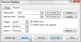
Figure 6-11: Use Replace options to change particular cell entries.
Be careful with global search-and-replace operations; they can really mess up a worksheet in a hurry if you inadvertently replace values, parts of formulas, or characters in titles and headings that you hadn’t intended to change. With this in mind, always follow one rule:
Never undertake a global search-and-replace operation on an unsaved worksheet.
Also, verify whether the Match Entire Cell Contents check box (displayed only when you click the Options button) is selected before you begin. You can end up with many unwanted replacements if you leave this check box unselected when you really only want to replace entire cell entries (rather than matching parts in cell entries).
If you do make a mess, immediately click the Undo button on the Quick Access toolbar or press Ctrl+Z to restore the worksheet.
To see each occurrence before you replace it, click the Find Next button or press Enter. Excel selects the next cell with the text or value you enter in the Find What text box. To have the program replace the selected text, click the Replace button. To skip this occurrence, click the Find Next button to continue the search. When you finish replacing occurrences, click the Close button to close the Find and Replace dialog box.
Doing Your Research
Excel 2013 includes the Research task pane that you can use to search for information using such online resources as Bing; Encarta Dictionary: English (North America); English, French, and Spanish Thesaurus; as well as Factiva iWorks and HighBeam Research. (Because these resources are online, to make use of the Research task pane, you must have Internet access available.)
To open the Research task pane (similar to the one shown in Figure 6-12), click the Research command button on the Ribbon’s Review tab or press Alt+RR. When you first open the Research pane, it is a floating pane that you can reposition anywhere in the worksheet by dragging it with the double white cross mouse or touch pointer. To dock the research pane at the left or right edge of the display screen, drag to one side or the other until it becomes docked in place.
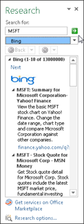
Figure 6-12: Looking up the stock quotes for Microsoft Corp (MSFT) with the Bing search engine in the Research task pane.
To look up something in the Research pane, select the cell in the worksheet that contains the word or phrase you want to research online or type the word or phrase directly into the Search For text box at the top of the Research pane. Then click the type of online reference to search on the Show Results From drop-down menu:
![]() All Reference Books to search for the word or phrase in any of the online reference books, such as the Encarta Dictionary: English (North America), Thesaurus: English (U.S.), and so on
All Reference Books to search for the word or phrase in any of the online reference books, such as the Encarta Dictionary: English (North America), Thesaurus: English (U.S.), and so on
![]() All Research Sites to look up the word or phrase in any online resource or any Web site such as Bing, Factiva iWorks, and HighBeam Research
All Research Sites to look up the word or phrase in any online resource or any Web site such as Bing, Factiva iWorks, and HighBeam Research
To start the online search, click the Start Searching button to the immediate right of the Search For text box (the green box with the right arrow. Excel then connects you to the designated online resources and displays the search results in the list box below. Figure 6-12, for example, shows the various stock quotes for Microsoft Corporation for the day and time I did the search using MSN Money Stock Quotes.
When you include Web sites in your search, you can visit particular sites by clicking their links in the Research task pane. When you do, Windows then launches your default Web browser (such as Internet Explorer or Firefox) and connects you to the linked page. To return to Excel after visiting a particular Web page, simply click the Close box in the upper-right corner of your Web browser’s window.
You can modify which online services are available for use in a search by clicking the Research Options link that appears at the very bottom of the Research task pane. When you click this link, Excel opens a Research Options dialog box that enables you to add or remove particular reference books and sites by selecting their check boxes.
Controlling Recalculation
Although extremely important, locating information in a worksheet is only part of keeping on top of the information in a worksheet. In really large workbooks that contain many completed worksheets, you may want to switch to manual recalculation so that you can control when the formulas in the worksheet are calculated. You need this kind of control when you find that Excel’s recalculation of formulas each time you enter or change information in cells has slowed the program’s response to a crawl. By holding off recalculations until you are ready to save or print the workbook, you find that you can work with Excel’s worksheets without interminable delays.
To put the workbook into manual recalculation mode, you select the Manual option on the Calculation Options’ button on the Formulas tab of the Ribbon (Alt+MXM). After switching to manual recalculation, Excel displays CALCULATE on the status bar whenever you make a change to the worksheet that somehow affects the current values of its formulas. Whenever Excel is in Calculate mode, you need to bring the formulas up-to-date in your worksheets before saving the workbook (as you would do before you print its worksheets).
To recalculate the formulas in a workbook when calculation is manual, press F9 or Ctrl+= (equal sign) or select the Calculate Now button (the one with a picture of a calculator in the upper-right corner of the Calculation group) on the Formulas tab (Alt+MB).
Excel then recalculates the formulas in all the worksheets of your workbook. If you made changes to only the current worksheet and you don’t want to wait around for Excel to recalculate every other worksheet in the workbook, you can restrict the recalculation to the current worksheet. Press Shift+F9 or click the Calculate Sheet button (the one with picture of a calculator under the worksheet in the lower-right corner of the Calculation group) on the Formulas tab (Alt+MJ).
If your worksheet contains data tables that perform different what-if scenarios (see Chapter 8 for details), you can have Excel automatically recalculate all parts of the worksheet except for those data tables by clicking Automatic Except Data Tables on the Calculation Options button’s drop-down menu on the Formulas tab (Alt+MXE).
To return a workbook to fully automatic recalculation mode, click the Automatic option on the Calculation Options button’s drop-down menu on the Formulas tab (Alt+MXA).
Putting on the Protection
After you more or less finalize a worksheet by checking out its formulas and proofing its text, you often want to guard against any unplanned changes by protecting the document.
Each cell in the worksheet can be locked or unlocked. By default, Excel locks all the cells in a worksheet so that, when you follow these steps, Excel locks the whole thing up tighter than a drum:
1. Click the Protect Sheet command button in the Changes group on the Review tab on Ribbon or press Alt+RPS.
Excel opens the Protect Sheet dialog box (see Figure 6-13) in which you select the check box options you want to be available when the protection is turned on in the worksheet. By default, Excel selects the Protect Worksheet and Contents of Locked Cells check box at the top of the Protect Sheet dialog box. Additionally, the program selects both the Select Locked Cells and Select Unlocked Cells check boxes in the Allow All Users of This Worksheet To list box below.

Figure 6-13: Protection options in the Protect Sheet dialog box.
2. (Optional) Click any of the check box options in the Allow All Users of This Worksheet To list box (such as Format Cells or Insert Columns) that you still want to be functional when the worksheet protection is operational.
3. If you want to assign a password that must be supplied before you can remove the protection from the worksheet, type the password in the Password to Unprotect Sheet text box.
4. Click OK or press Enter.
If you type a password in the Password to Unprotect Sheet text box, Excel opens the Confirm Password dialog box. Re-enter the password in the Reenter Password to Proceed text box exactly as you typed it in the Password to Unprotect Sheet text box in the Protect Sheet dialog box and then click OK or press Enter.
If you want to go a step further and protect the layout of the worksheets in the workbook, you protect the entire workbook as follows:
1. Click the Protect Workbook command button in the Changes group on the Ribbon’s Review tab or press Alt+RPW.
Excel opens the Protect Structure and Windows dialog box, where the Structure check box is selected and the Windows check box is not selected. With the Structure check box selected, Excel won’t let you mess around with the sheets in the workbook (by deleting them or rearranging them). If you want to protect any windows that you set up (as I describe in Chapter 7), you need to select the Windows check box as well.
2. To assign a password that must be supplied before you can remove the protection from the worksheet, type the password in the Password (Optional) text box.
3. Click OK or press Enter.
If you type a password in the Password (Optional) text box, Excel opens the Confirm Password dialog box. Re-enter the password in the Reenter Password to Proceed text box exactly as you typed it into the Password (Optional) text box in the Protect Structure and Windows dialog box and then click OK or press Enter.
Selecting the Protect Sheet command makes it impossible to make further changes to the contents of any of the locked cells in that worksheet, except for those options that you specifically exempt in the Allow All Users of This Worksheet To list box. (See Step 2 in the first set of steps in this section.) Selecting the Protect Workbook command makes it impossible to make further changes to the layout of the worksheets in that workbook.
Excel displays an alert dialog box with the following message when you try to edit or replace an entry in a locked cell:
The cell or chart you are trying to change is on a
protected sheet.
To make changes, click Unprotect Sheet in the Review
Tab (you might need a password).
Usually, your intention in protecting a worksheet or an entire workbook is not to prevent all changes but to prevent changes in certain areas of the worksheet. For example, in a budget worksheet, you may want to protect all the cells that contain headings and formulas but allow changes in all the cells where you enter the budgeted amounts. That way, you can’t inadvertently wipe out a title or formula in the worksheet simply by entering a value in the wrong column or row (a common occurrence).
To leave certain cells unlocked so that you can still change them after protecting the worksheet or workbook, select all the cells as the cell selection, open the Format Cells dialog box (Ctrl+1), and then click the Locked check box on the Protection tab to remove its check mark. Then, after unlocking the cells that you still want to be able to change, protect the worksheet as described earlier.
To remove protection from the current worksheet or workbook document so that you can again make changes to its cells (whether locked or unlocked), click the Unprotect Sheet or the Unprotect Workbook command button in the Changes group on the Ribbon’s Review tab (or press Alt+RPS and Alt+RPW, respectively). If you assign a password when protecting the worksheet or workbook, you must then reproduce the password exactly as you assigned it (including any case differences) in the Password text box of the Unprotect Sheet or Unprotect Workbook dialog box.
You can also protect a worksheet or your workbook from Excel Info screen in the Backstage by clicking the Protect Workbook button (Alt+FIP). Clicking this button opens a menu of protection options, including among others, the familiar Protect Current Sheet to prevent changes to the current worksheet in the Protect Sheet dialog box and Protect Workbook Structure to changes to worksheets and or windows set up in the current workbook in the Protect Structure and Windows dialog box.