Chapter 2

Creating a Spreadsheet from Scratch

In This Chapter

Starting a new workbook

Entering the three different types of data in a worksheet

Creating simple formulas by hand

Fixing your data-entry boo-boos

Using the AutoCorrect feature

Using the AutoFill and Flash Fill features to complete a series of entries

Entering and editing formulas containing built-in functions

Totaling columns and rows of numbers with the AutoSum button

Saving your precious work and recovering workbooks after a computer crash

After you know how to launch Excel 2013, it’s time to find out how not to get yourself into trouble when actually using it! In this chapter, you find out how to put all kinds of information into all those little, blank worksheet cells I describe in Chapter 1. Here you find out about the Excel AutoCorrect and AutoComplete features and how they can help cut down on errors and speed up your work. You also get some basic pointers on other smart ways to minimize the drudgery of data entry, such as filling out a series of entries with the AutoFill and Flash Fill features as well as entering the same thing in a bunch of cells all at the same time.

After discovering how to fill up a worksheet with all this raw data, you find out what has to be the most important lesson of all — how to save all that information on disk so that you don’t ever have to enter the stuff again!

So What Ya Gonna Put in That New Workbook of Yours?

When you launch Excel 2013, an Excel 2013 start screen similar to the one shown in Figure 2-1 appears separated into two panes. In the left pane, Excel lists the names of recently edited workbooks (if any). Below that, the left pane contains an Open Other Workbooks link.

In the pane on the right side of the start screen, Excel displays thumbnail images of various templates that you can use when starting a new workbook. Templates create new workbooks that follow a particular form such as a budget or inventory list. These new workbooks generated from a template contain ready-made tables and lists often with sample data and headings that you can then edit and change as needed. Then, when you finish, you can save the new customized workbook with a new filename.

Figure 2-1: The Excel 2013 start screen that appears when you first launch the program.

The template thumbnails begin with a Blank Workbook template immediately followed by a Take a Tour template. After that, you find thumbnails for a bunch of commonly used workbooks, ranging from budgets to calendars. If none of the example workbooks offered by this list of templates suits your needs, you can use the Search Online Templates text box to find many more templates of a specific type. Right below, you can also click any of the links (Budget, Invoice, Calendars, and so on) in the Suggested Searches to bring up and display a whole hoard of templates of a particular type.

I highly recommend opening the Take a Tour template at some point early in your exploration of Excel 2013. When you click its template thumbnail, Excel immediately opens a new Welcome to Excel1 workbook replete with five worksheets: Start, Fill, Analyze, Chart, and Learn More. The Fill worksheet lets you try out the new Flash Fill feature discussed later in this chapter. The Analyze worksheet lets you experiment with the new Quick Analysis feature covered in Chapter 3. The Chart worksheet lets you test the new Recommended Charts feature discussed in Chapter 10. After playing with any or all of these new features, you can close the Welcome to Excel1 workbook without saving your changes.

When you select one of the template thumbnails in the Excel 2013 start screen other than Blank Workbook and Take a Tour, Excel opens a dialog box that contains a larger version of the template thumbnail along with the name, a brief description, download size, and rating. To then download the template and create a new workbook from it in Excel, you click the Create button. If, on perusing the information in this dialog box, you decide that this isn’t the template you want to use after all, click the Close button or simply press Esc.

To start a new workbook devoid of any labels and data, you click the Blank Workbook template in the Excel 2013 start screen. When you do, Excel opens a new workbook automatically named Book1. This workbook contains a single blank worksheet, automatically named Sheet1. To begin to work on a new spreadsheet, you simply start entering information in the Sheet1 worksheet of the Book1 workbook window.

The ins and outs of data entry

Here are a few simple guidelines (a kind of data-entry etiquette, if you will) to keep in mind when you create a spreadsheet in Sheet1 of your new blank workbook:

Whenever you can, organize your information in tables of data that use adjacent (neighboring) columns and rows. Start the tables in the upper-left corner of the worksheet and work your way down the sheet, rather than across the sheet, whenever possible. When it’s practical, separate each table by no more than a single column or row.

When you set up these tables, don’t skip columns and rows just to “space out” the information. In Chapter 3, you see how to place as much white space as you want between information in adjacent columns and rows by widening columns, heightening rows, and changing the alignment.

Reserve a single column at the left edge of the table for the table’s row headings.

Reserve a single row at the top of the table for the table’s column headings.

If your table requires a title, put the title in the row above the column headings. Put the title in the same column as the row headings. You can get information on how to center this title across the columns of the entire table in Chapter 3.

In Chapter 1, I make a big deal about how big each of the worksheets in a workbook is. You may wonder why I’m now on your case about not using that space to spread out the data that you enter into it. After all, given all the real estate that comes with each Excel worksheet, you’d think conserving space would be one of the last things you’d have to worry about.

You’d be 100 percent correct . . . except for one little, itty-bitty thing: Space conservation in the worksheet equals memory conservation. You see, while a table of data grows and expands into columns and rows in new areas of the worksheet, Excel decides that it had better reserve a certain amount of computer memory and hold it open just in case you go crazy and fill that area with cell entries. Therefore, if you skip columns and rows that you really don’t need to skip (just to cut down on all that cluttered data), you end up wasting computer memory that could store more information in the worksheet.

You must remember this . . .

Now you know: The amount of computer memory available to Excel determines the ultimate size of the spreadsheet you can build, not the total number of cells in the worksheets of your workbook. When you run out of memory, you’ve effectively run out of space — no matter how many columns and rows are still available. To maximize the information you can get into a single worksheet, always adopt the “covered wagon” approach to worksheet design by keeping your data close together.

Doing the Data-Entry Thing

Begin by reciting (in unison) the basic rule of worksheet data entry. All together now:

To enter data in a worksheet, position the cell pointer in the cell where you want the data and then begin typing the entry.

Before you can position the cell pointer in the cell where you want the entry, Excel must be in Ready mode (look for Ready as the Program indicator at the beginning of the Status bar). When you start typing the entry, however, Excel goes through a mode change from Ready to Enter mode (and Enter replaces Ready as the Program indicator). If you’re not in Ready mode, try pressing Esc on your keyboard.

And if you’re doing data entry on a worksheet on a device that doesn’t have a physical keyboard, for heaven’s sake, open the virtual keyboard and keep it open (preferably floating) in the Excel window during the whole time you’re doing data entry. (See “Tips on using a virtual keyboard” in Chapter 1 for details on displaying and using the virtual keyboard on a touchscreen device.)

As soon as you begin typing in Enter mode, the characters that you type in a cell in the worksheet area simultaneously appear on the Formula bar near the top of the screen. Typing something in the current cell also triggers a change to the Formula bar because two new buttons, Cancel and Enter, appear between the Name box drop-down button and the Insert Function button.

As you continue to type, Excel displays your progress on the Formula bar and in the active cell in the worksheet (see Figure 2-2). However, the insertion point (the flashing vertical bar that acts as your cursor) displays only at the end of the characters displayed in the cell.

Figure 2-2: What you type appears both in the current cell and on the Formula bar.

After you finish typing your cell entry, you still have to get it into the cell so that it stays put. When you do this, you also change the program from Enter mode back to Ready mode so that you can move the cell pointer to another cell and, perhaps, enter or edit the data there.

To complete your cell entry and, at the same time, get Excel out of Enter mode and back into Ready mode, you can select the Enter button on the Formula bar or press the Enter key or one of the arrow keys (, , →, or ←) on your physical or virtual keyboard. You can also press the Tab key or Shift+Tab keys to complete a cell entry.

When you complete a cell entry with any of the keyboard keys — Enter, Tab, Shift+Tab, or any of the arrow keys — you not only complete the entry in the current cell but get the added advantage of moving the cell pointer to a neighboring cell in the worksheet that requires editing or data entry.

Now, even though each of these alternatives gets your text into the cell, each does something a little different afterward, so please take note:

If you select the Enter button (the one with the check mark) on the Formula bar, the text goes into the cell, and the cell pointer just stays in the cell containing the brand-new entry.

If you press the Enter key on your physical or virtual keyboard, the text goes into the cell, and the cell pointer moves down to the cell below in the next row.

If you press one of the arrow keys, the text goes into the cell, and the cell pointer moves to the next cell in the direction of the arrow. Press , and the cell pointer moves below in the next row just as it does when you finish off a cell entry with the Enter key. Press → to move the cell pointer right to the cell in the next column; press ← to move the cell pointer left to the cell in the previous column; and press to move the cell pointer up to the cell in the next row above.

If you press Tab, the text goes into the cell, and the cell pointer moves to the adjacent cell in the column on the immediate right (the same as pressing the → key). If you press Shift+Tab, the cell pointer moves to the adjacent cell in the column on the immediate left (the same as pressing the ← key) after putting in the text.

No matter which of the methods you choose when putting an entry in its place, as soon as you complete your entry in the current cell, Excel deactivates the Formula bar by removing the Cancel and Enter buttons. Thereafter, the data you entered continues to appear in the cell in the worksheet (with certain exceptions that I discuss later in this chapter), and every time you put the cell pointer into that cell, the data will reappear on the Formula bar as well.

---

---

If, while still typing an entry or after finishing typing but prior to completing the entry, you realize that you’re just about to stick it in the wrong cell, you can clear and deactivate the Formula bar by selecting the Cancel button (the one with the X in it) or by pressing Esc on your keyboard. If, however, you don’t realize that you had the wrong cell until after you enter your data there, you have to either move the entry to the correct cell (something you find out how to do in Chapter 4) or delete the entry (see Chapter 4) and then re-enter the data in the correct cell.

It Takes All Types

Unbeknownst to you while you go about happily entering data in your spreadsheet, Excel constantly analyzes the stuff you type and classifies it into one of three possible data types: a piece of text, a value, or a formula.

If Excel finds that the entry is a formula, the program automatically calculates the formula and displays the computed result in the worksheet cell (you continue to see the formula itself, however, on the Formula bar). If Excel is satisfied that the entry does not qualify as a formula (I give you the qualifications for an honest-to-goodness formula a little later in this chapter), the program then determines whether the entry should be classified as text or as a value.

Excel makes this distinction between text and values so that it knows how to align the entry in the worksheet. It aligns text entries with the left edge of the cell and values with the right edge. Because most formulas work properly only when they are fed values, by differentiating text from values, the program knows which will and will not work in the formulas that you build. Suffice to say that you can foul up your formulas but good if they refer to any cells containing text where Excel expects values to be.

The telltale signs of text

A text entry is simply an entry that Excel can’t pigeonhole as either a formula or value. This makes text the catchall category of Excel data types. As a practical rule, most text entries (also known as labels) are a combination of letters and punctuation or letters and numbers. Text is used mostly for titles, headings, and notes in the worksheet.

You can tell right away whether Excel has accepted a cell entry as text because text entries automatically align at the left edge of their cells. If the text entry is wider than the cell can display, the data spills into the neighboring cell or cells on the right, as long as those cells remain blank.

If, sometime later, you enter information in a cell that contains spillover text from a cell to its left, Excel cuts off the spillover of the long text entry (see Figure 2-3). Not to worry: Excel doesn’t actually lop these characters off the cell entry — it simply shaves the display to make room for the new entry. To redisplay the seemingly missing portion of the long text entry, you have to widen the column that contains the cell where the text is entered. (To find out how to do this, skip ahead to Chapter 3.)

Figure 2-3: Entries in cells to the right cut off the spillover text in cells on the left.

How Excel evaluates its values

Values are the building blocks of most of the formulas that you create in Excel. As such, values come in two flavors: numbers that represent quantities (14 stores or $140,000 dollars) and numbers that represent dates (July 30, 1995) or times (2 p.m.).

You can tell whether Excel has accepted your entry as a value because values automatically align at the right edge of their cells. If the value that you enter is wider than the column containing the cell can display, Excel automatically converts the value to (of all things) scientific notation. To restore a value that’s been converted into that weird scientific notation stuff to a regular number, simply widen the column for that cell. (Read how in Chapter 3.)

Verifying Excel’s got your number

When building a new worksheet, you’ll probably spend a lot of your time entering numbers, representing all types of quantities from money that you made (or lost) to the percentage of the office budget that went to coffee and donuts. (You mean you don’t get donuts?)

To enter a numeric value that represents a positive quantity, like the amount of money you made last year, just select a cell, type the numbers — for example, 459600 — and complete the entry in the cell by clicking the Enter button, pressing the Enter key, and so on. To enter a numeric value that represents a negative quantity, such as the amount of money the office spent on coffee and donuts last year, begin the entry with the minus sign or hyphen (–) before typing the numbers and then complete the entry. For example, –175 (that’s not too much to spend on coffee and donuts when you just made $459,600).

---

---

If you’re trained in accounting, you can enclose the negative number (that’s expense to you) in parentheses. You’d enter it like this: (175). If you go to all the trouble to use parentheses for your negatives (expenses), Excel goes ahead and automatically converts the number so that it begins with a minus sign; if you enter (175) in the Coffee and Donut expense cell, Excel spits back –175. (Relax, you can find out how to get your beloved parentheses back for the expenses in your spreadsheet in Chapter 3.)

With numeric values that represent dollar amounts, like the amount of money you made last year, you can include dollar signs ($) and commas (,) just as they appear in the printed or handwritten numbers you’re working from. Just be aware that when you enter a number with commas, Excel assigns a number format to the value that matches your use of commas. (For more information on number formats and how they are used, see Chapter 3.) Likewise, when you preface a financial figure with a dollar sign, Excel assigns an appropriate dollar-number format to the value (one that automatically inserts commas between the thousands).

When entering numeric values with decimal places, use the period as the decimal point. When you enter decimal values, the program automatically adds a zero before the decimal point (Excel inserts 0.34 in a cell when you enter .34) and drops trailing zeros entered after the decimal point (Excel inserts 12.5 in a cell when you enter 12.50).

If you don’t know the decimal equivalent for a value that contains a fraction, you can just go ahead and enter the value with its fraction. For example, if you don’t know that 2.1875 is the decimal equivalent for 2³⁄₁₆, just type 2 ³⁄₁₆ (making sure to add a space between the 2 and 3) in the cell. After completing the entry, when you put the cell pointer in that cell, you see 2³⁄₁₆ in the cell of the worksheet, but 2.1875 appears on the Formula bar. As you see in Chapter 3, it’s then a simple trick to format the display of 2³⁄₁₆ in the cell so that it matches the 2.1875 on the Formula bar.

If you need to enter simple fractions, such as ³⁄₄ or ⁵⁄₈, you must enter them as a mixed number preceded by zero; for example, enter 0 ³/₄ or 0 ⁵/₈ (be sure to include a space between the zero and the fraction). Otherwise, Excel thinks that you’re entering the dates March 4 (3/4) and May 8 (5/8).

When entering in a cell a numeric value that represents a percentage (so much out of a hundred), you have this choice:

You can either divide the number by 100 and enter the decimal equivalent (by moving the decimal point two places to the left like your teacher taught you; for example, enter .12 for 12 percent).

You can enter the number with the percent sign (for example, enter 12%).

Either way, Excel stores the decimal value in the cell (0.12 in this example). If you use the percent sign, Excel assigns a percentage-number format to the value in the worksheet so that it appears as 12%.

How to fix your decimal places (when you don’t even know they’re broken)

If you find that you need to enter a whole slew of numbers that use the same number of decimal places, you can turn on Excel’s Fixed Decimal setting and have the program enter the decimals for you. This feature really comes in handy when you have to enter hundreds of financial figures that all use two decimal places (for example, for the number of cents).

To fix the number of decimal places in a numeric entry, follow these steps:

1. Choose File⇒Options⇒Advanced or press Alt+FTA.

The Advanced tab of the Excel Options dialog box opens.

2. Select the Automatically Insert a Decimal Point check box in the Editing Options section to fill it with a check mark.

By default, Excel fixes the decimal place two places to the left of the last number you type. To change the default Places setting, go to Step 3; otherwise move to Step 4.

3. (Optional) Select or enter a new number in the Places text box or use the spinner buttons to change the value.

For example, you could change the Places setting to 3 to enter numbers with the following decimal placement: 00.000.

4. Click OK or press Enter.

Excel displays the Fixed Decimal status indicator on the Status bar to let you know that the Fixed Decimal feature is now active.

---

---

After fixing the decimal place in numeric values, Excel automatically adds a decimal point to any numeric value that you enter using the number of places you selected; all you do is type the digits and complete the entry in the cell. For example, to enter the numeric value 100.99 in a cell after fixing the decimal point to two places, type the digits 10099 without adding any period for a decimal point. When you complete the cell entry, Excel automatically inserts a decimal point two places from the right in the number you typed, leaving 100.99 in the cell.

When you’re ready to return to normal data entry for numerical values (where you enter any decimal points yourself), open the Advanced tab of the Excel Options dialog box (Alt+FTA), select the Automatically Insert a Decimal Point check box again, this time to clear it, and then click OK or press Enter. Excel removes the Fixed Decimal indicator from the Status bar.

Tapping on the old ten-key

You can make the Fixed Decimal feature work even better when entering numeric data on a physical keyboard that has a separate ten-key numeric keypad. All you do is select the block of cells where you want to enter numbers (see “Entries all around the block,” later in this chapter) and then press Num Lock so that you can enter all the data for this cell selection from the numeric keypad (à la ten-key adding machine).

Using this approach, all you have to do to enter the range of values in each cell is type the number’s digits and press Enter on the numeric keypad. Excel inserts the decimal point in the proper place while it moves the cell pointer down to the next cell. Even better, when you finish entering the last value in a column, pressing Enter automatically moves the cell pointer to the cell at the top of the next column in the selection.

Look at Figures 2-4 and 2-5 to see how you can make the ten-key method work for you. In Figure 2-4, the Fixed Decimal feature is turned on (using the default of two decimal places), and the block of cells from B3 through D9 are selected. You also see that six entries have already been made in cells B3 through B8 and a seventh, 30834.63, is about to be completed in cell B9. To make this entry when the Fixed Decimal feature is on, you simply type 3083463 from the numeric keypad.

In Figure 2-5, check out what happens when you press Enter (on either the regular keyboard or the numeric keypad). Not only does Excel automatically add the decimal point to the value in cell B9, but it also moves the cell pointer up and over to cell C3 where you can continue entering the values for this column.

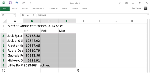
Figure 2-4: To enter the value 30834.63 in cell B9, type 3083463 and press Enter.

Figure 2-5: Press Enter to complete the 30834.63 entry in cell B9. Excel automatically moves the cell pointer up and over to cell C3.

Entering dates with no debate

At first look, it may strike you a bit odd to enter dates and times as values in the cells of a worksheet rather than text. The reason for this is simple, really: Dates and times entered as values can be used in formula calculations, whereas dates and times entered as text cannot. For example, if you enter two dates as values, you can then set up a formula that subtracts the more recent date from the older date and returns the number of days between them. This kind of thing just couldn’t happen if you were to enter the two dates as text entries.

Excel determines whether the date or time that you type is a value or text by the format that you follow. If you follow one of Excel’s built-in date-and-time formats, the program recognizes the date or time as a value. If you don’t follow one of the built-in formats, the program enters the date or time as a text entry — it’s as simple as that.

Excel recognizes the following time formats:

3 AM or 3 PM

3 A or 3 P (upper- or lowercase a or p — Excel inserts 3:00 AM or 3:00 PM)

3:21 AM or 3:21 PM (upper- or lowercase am or pm)

3:21:04 AM or 3:21:04 PM (upper- or lowercase am or pm)

15:21

15:21:04

Excel isn’t fussy, so you can enter the AM or PM designation in the date in any manner — uppercase letters, lowercase letters, or even a mix of the two.

Excel knows the following date formats. (Month abbreviations always use the first three letters of the name of the month: Jan, Feb, Mar, and so forth.)

November 6, 2012 or November 6, 12 (appear in cell as 6-Nov-12

11/6/12 or 11-6-12 (appear in cell as 11/6/2012)

6-Nov-12 or 6/Nov/12 or even 6Nov12 (all appear in cell as 6-Nov-12)

11/6 or 6-Nov or 6/Nov or 6Nov (all appear in cell as 6-Nov)

Nov-06 or Nov/06 or Nov06 (all appear in cell as 6-Nov)

---

---

Make it a date in the 21st Century

Contrary to what you might think, when entering dates in the 21st Century, you need to enter only the last two digits of the year. For example, to enter the date January 6, 2012, in a worksheet, I enter 1/6/12 in the target cell. Likewise, to put the date February 15, 2013, in a worksheet, I enter 2/15/13 in the target cell.

Entering only the last two digits of dates in the 21st Century works only for dates in the first three decades of the new century (2000 through 2029). To enter dates for the years 2030 on, you need to input all four digits of the year.

This also means, however, that to put in dates in the first three decades of the 20th Century (1900 through 1929), you must enter all four digits of the year. For example, to put in the date July 21, 1925, you have to enter 7/21/1925 in the target cell. Otherwise, if you enter just the last two digits (25) for the year part of the date, Excel enters a date for the year 2025 and not 1925!

Excel 2013 always displays all four digits of the year in the cell and on the Formula bar even when you only enter the last two. For example, if you enter 11/06/12 in a cell, Excel automatically displays 11/6/2012 in the worksheet cell (and on the Formula bar when that cell is current).

Therefore, by looking at the Formula bar, you can always tell when you’ve entered a 20th rather than a 21st Century date in a cell even if you can’t keep straight the rules for when to enter just the last two digits rather than all four. (Read Chapter 3 for information on how to format your date entries so that only the last digits display in the worksheet.)

For information on how to perform simple arithmetic operations between the dates and time you enter in a worksheet and have the results make sense, see the information about dates in Chapter 3.

Fabricating those fabulous formulas!

As entries go in Excel, formulas are the real workhorses of the worksheet. If you set up a formula properly, it computes the correct answer when you enter the formula into a cell. From then on, the formula stays up to date, recalculating the results whenever you change any of the values that the formula uses.

You let Excel know that you’re about to enter a formula (rather than some text or a value), in the current cell by starting the formula with the equal sign (=). Most simple formulas follow the equal sign with a built-in function, such as SUM or AVERAGE. (See the section “Inserting a function into a formula with the Insert Function button,” later in this chapter, for more information on using functions in formulas.) Other simple formulas use a series of values or cell references that contain values separated by one or more of the following mathematical operators:

+ (plus sign) for addition

– (minus sign or hyphen) for subtraction

* (asterisk) for multiplication

/ (slash) for division

^ (caret) for raising a number to an exponential power

For example, to create a formula in cell C2 that multiplies a value entered in cell A2 by a value in cell B2, enter the following formula in cell C2: =A2*B2.

To enter this formula in cell C2, follow these steps:

1. Select cell C2.

2. Type the entire formula =A2*B2 in the cell.

3. Press Enter.

Or

1. Select cell C2.

2. Type = (equal sign).

3. Select cell A2 in the worksheet by using the mouse or the keyboard.

This action places the cell reference A2 in the formula in the cell (as shown in Figure 2-6).

Figure 2-6: To start the formula, type = and then select cell A2.

4. Type * (Shift+8 on the top row of the keyboard).

The asterisk is used for multiplication rather than the × symbol you used in school.

5. Select cell B2 in the worksheet with the mouse, keyboard, or by tapping it on the screen (when using a touchscreen device).

This action places the cell reference B2 in the formula (as shown in Figure 2-7).

6. Click the Enter button on the Formula bar to complete the formula entry while keeping the cell pointer in cell C2.

Excel displays the calculated answer in cell C2 and the formula =A2*B2 in the Formula bar (as shown in Figure 2-8).

When you finish entering the formula =A2*B2 in cell C2 of the worksheet, Excel displays the calculated result, depending on the values currently entered in cells A2 and B2. The major strength of the electronic spreadsheet is the capability of formulas to change their calculated results automatically to match changes in the cells referenced by the formulas.

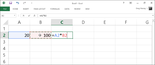
Figure 2-7: To complete the second part of the formula, type * and select cell B2.

Figure 2-8: Select the Enter button, and Excel displays the answer in cell C2 while the formula appears in the Formula bar above.

Now comes the fun part: After creating a formula like the preceding one that refers to the values in certain cells (rather than containing those values itself), you can change the values in those cells, and Excel automatically recalculates the formula, using these new values and displaying the updated answer in the worksheet! Using the example shown in Figure 2-8, suppose that you change the value in cell B2 from 100 to 50. The moment that you complete this change in cell B2, Excel recalculates the formula and displays the new answer, 1000, in cell C2.

If you want it, just point it out

The method of selecting the cells you use in a formula, rather than typing their cell references, is pointing. On most devices on which you’re running Excel 2013, pointing is quicker than typing and certainly reduces the risk that you might mistype a cell reference. When you type a cell reference, you can easily type the wrong column letter or row number and not realize your mistake by looking at the calculated result returned in the cell. But when you directly select the cell that you want to use in a formula (by clicking or tapping it or even using the arrow keys to move the cell cursor to it), you have less chance of entering the wrong cell reference.

On a small handheld device with a tiny touchscreen such as a smartphone, sliding to scroll to the proper column and row and then tapping the cell to select and add its reference to a new formula may be even more challenging than typing the formula’s cell references on the device’s virtual keyboard. This is when I recommend typing instead of pointing for creating new formulas. Just be aware that when you type the first letter of your cell’s column reference into a formula, Excel automatically displays a list of all the built-in functions whose names start with that letter. This list immediately disappears as soon as you type the second letter of the column (if the cell has one) or the first digit of its row number. Also, be sure to double-check that the cell references you type into the formula refer to the cells you really want to use.

Altering the natural order of operations

Many formulas that you create perform more than one mathematical operation. Excel performs each operation, moving from left to right, according to a strict pecking order (the natural order of arithmetic operations). In this order, multiplication and division pull more weight than addition and subtraction and, therefore, perform first, even if these operations don’t come first in the formula (when reading from left to right).

Consider the series of operations in the following formula:

=A2+B2*C2

If cell A2 contains the number 5, B2 contains the number 10, and C2 contains the number 2, Excel evaluates the following formula:

=5+10*2

In this formula, Excel multiplies 10 times 2 to equal 20 and then adds this result to 5 to produce the result 25.

If you want Excel to perform the addition between the values in cells A2 and B2 before the program multiplies the result by the value in cell C2, enclose the addition operation in parentheses as follows:

=(A2+B2)*C2

The parentheses around the addition tell Excel that you want this operation performed before the multiplication. If cell A2 contains the number 5, B2 contains the number 10, and C2 contains the number 2, Excel adds 5 and 10 to equal 15 and then multiplies this result by 2 to produce the result 30.

In fancier formulas, you may need to add more than one set of parentheses, one within another (like the wooden Russian dolls that nest within each other) to indicate the order in which you want the calculations to take place. When nesting parentheses, Excel first performs the calculation contained in the most inside pair of parentheses and then uses that result in further calculations as the program works its way outward. For example, consider the following formula:

=(A4+(B4–C4))*D4

Excel first subtracts the value in cell C4 from the value in cell B4, adds the difference to the value in cell A4, and then finally multiplies that sum by the value in D4.

Without the additions of the two sets of nested parentheses, left to its own devices, Excel would first multiply the value in cell C4 by that in D4, add the value in A4 to that in B4, and then perform the subtraction.

Don’t worry too much when nesting parentheses in a formula if you don’t pair them properly so that you have a right parenthesis for every left parenthesis in the formula. If you do not include a right parenthesis for every left one, Excel displays an alert dialog box that suggests the correction needed to balance the pairs. If you agree with the program’s suggested correction, you simply click the Yes button. However, be sure that you only use parentheses: ( ). Excel balks at the use of brackets — [ ] — or braces — { } — in a formula by giving you an Error alert box.

Formula flub-ups

Under certain circumstances, even the best formulas can appear to have freaked out after you get them in your worksheet. You can tell right away that a formula’s gone haywire because instead of the nice calculated value you expected to see in the cell, you get a strange, incomprehensible message in all uppercase letters beginning with the number sign (#) and ending with an exclamation point (!) or, in one case, a question mark (?). This weirdness, in the parlance of spreadsheets, is as an error value. Its purpose is to let you know that some element — either in the formula itself or in a cell referred to by the formula — is preventing Excel from returning the anticipated calculated value.

When one of your formulas returns one of these error values, an alert indicator (in the form of an exclamation point in a diamond) appears to the left of the cell when it contains the cell pointer, and the upper-left corner of the cell contains a tiny green triangle. When you position the mouse pointer on this alert indicator, Excel displays a brief description of the formula error and adds a drop-down button to the immediate right of its box. When you click this button, a pop-up menu appears with a number of related options. To access online help on this formula error, including suggestions on how to get rid of the error, click the Help on This Error item on this pop-up menu.

The worst thing about error values is that they can contaminate other formulas in the worksheet. If a formula returns an error value to a cell and a second formula in another cell refers to the value calculated by the first formula, the second formula returns the same error value, and so on down the line.

After an error value shows up in a cell, you have to discover what caused the error and edit the formula in the worksheet. In Table 2-1, I list some error values that you might run into in a worksheet and then explain the most common causes.

Table 2-1 Error Values That You May Encounter from Faulty Formulas

What Shows Up in the Cell	What’s Going On Here?
#DIV/0!	Appears when the formula calls for division by a cell that either contains the value 0 or, as is more often the case, is empty. Division by zero is a no-no in mathematics.
#NAME?	Appears when the formula refers to a range name (see Chapter 6 for info on naming ranges) that doesn’t exist in the worksheet. This error value appears when you type the wrong range name or fail to enclose in quotation marks some text used in the formula, causing Excel to think that the text refers to a range name.
#NULL!	Appears most often when you insert a space (where you should have used a comma) to separate cell references used as arguments for functions.
#NUM!	Appears when Excel encounters a problem with a number in the formula, such as the wrong type of argument in an Excel function or a calculation that produces a number too large or too small to be represented in the worksheet.
#REF!	Appears when Excel encounters an invalid cell reference, such as when you delete a cell referred to in a formula or paste cells over the cells referred to in a formula.
#VALUE!	Appears when you use the wrong type of argument or operator in a function, or when you call for a mathematical operation that refers to cells that contain text entries.

Fixing Those Data Entry Flub-Ups

We all wish we were perfect, but alas, because so few of us are, we are best off preparing for those inevitable times when we mess up. When entering vast quantities of data, it’s easy for those nasty little typos to creep into your work. In your pursuit of the perfect spreadsheet, here are things you can do. First, get Excel to correct certain data entry typos automatically when they happen with its AutoCorrect feature. Second, manually correct any disgusting little errors that get through, either while you’re still in the process of making the entry in the cell or after the entry has gone in.

You really AutoCorrect that for me

The AutoCorrect feature is a godsend for those of us who tend to make the same stupid typos over and over. With AutoCorrect, you can alert Excel 2013 to your own particular typing gaffes and tell the program how it should automatically fix them for you.

When you first install Excel, the AutoCorrect feature already knows to automatically correct two initial capital letters in an entry (by lowercasing the second capital letter), to capitalize the name of the days of the week, and to replace a set number of text entries and typos with particular substitute text.

You can add to the list of text replacements at any time when using Excel. These text replacements can be of two types: typos that you routinely make along with the correct spelling, and abbreviations or acronyms that you type all the time along with their full forms.

To add to the replacements

1. Choose File⇒Options⇒Proofing or press Alt+FTP and then click the AutoCorrect Options button or press Alt+A.

Excel opens the AutoCorrect dialog box shown in Figure 2-9.

2. On the AutoCorrect tab in this dialog box, enter the typo or abbreviation in the Replace text box.

3. Enter the correction or full form in the With text box.

4. Click the Add button or press Enter to add the new typo or abbreviation to the AutoCorrect list.

5. Click the OK button to close the AutoCorrect dialog box.

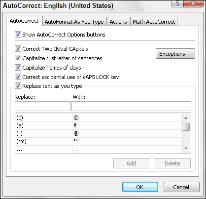
Figure 2-9: Use the Replace and With options in the AutoCorrect dialog box to add all typos and abbreviations you want Excel to automatically correct or fill out.

Cell editing etiquette

Despite the help of AutoCorrect, some mistakes are bound to get you. How you correct them really depends upon whether you notice before or after completing the cell entry.

If you catch the mistake before you complete an entry, you can delete it by pressing your Backspace key until you remove all the incorrect characters from the cell. Then you can retype the rest of the entry or the formula before you complete the entry in the cell.

If you don’t discover the mistake until after you’ve completed the cell entry, you have a choice of replacing the whole thing or editing just the mistakes.

When dealing with short entries, you’ll probably want to take the replacement route. To replace a cell entry, position the cell pointer in that cell, type your replacement entry, and then click the Enter button or press Enter.

When the error in an entry is relatively easy to fix and the entry is on the long side, you’ll probably want to edit the cell entry rather than replace it. To edit the entry in the cell, simply double-click or double-tap the cell or select the cell and then press F2.

Doing either one reactivates the Formula bar by displaying the Enter and Cancel buttons once again and placing the insertion point in the cell entry in the worksheet. (If you double-click or double-tap, the insertion point positions itself wherever you click; press F2, and the insertion point positions itself after the last character in the entry.)

Notice also that the mode indicator changes to Edit. While in this mode, you can use the mouse or the arrow keys to position the insertion point at the place in the cell entry that needs fixing.

In Table 2-2, I list the keystrokes that you can use to reposition the insertion point in the cell entry and delete unwanted characters. If you want to insert new characters at the insertion point, simply start typing. If you want to delete existing characters at the insertion point while you type new ones, press the Insert key on your keyboard to switch from the normal insert mode to overtype mode. To return to normal insert mode, press Insert a second time. When you finish making corrections to the cell entry, you must complete the edits by pressing Enter before Excel updates the contents of the cell.

While Excel is in Edit mode, you must re-enter the edited cell contents by either clicking the Enter button or pressing Enter. You can use the arrow keys as a way to complete an entry only when the program is in Enter mode. When the program is in Edit mode, the arrow keys move the insertion point only through the entry that you’re editing, not to a new cell.

Table 2-2 Keystrokes for Fixing Those Cell Entry Flub-Ups

Keystroke	What the Keystroke Does
Delete	Deletes the character to the right of the insertion point
Backspace	Deletes the character to the left of the insertion point
→	Positions the insertion point one character to the right
←	Positions the insertion point one character to the left
	Positions the insertion point, when it is at the end of the cell entry, to its preceding position to the left
End or	Moves the insertion point after the last character in the cell entry
Home	Moves the insertion point in front of the first character of the cell entry
Ctrl+→	Positions the insertion point in front of the next word in the cell entry
Ctrl+←	Positions the insertion point in front of the preceding word in the cell entry
Insert	Switches between insert and overtype mode

---

---

Taking the Drudgery out of Data Entry

Before leaving the topic of data entry, I feel duty-bound to cover some of the shortcuts that really help to cut down on the drudgery of this task. These data-entry tips include the AutoComplete, AutoFill, and Flash Fill features as well as doing data entry in a preselected block of cells and making the same entry in a bunch of cells all at the same time.

I’m just not complete without you

The AutoComplete feature in Excel 2013 is not something you can do anything about, just something to be aware of while you enter your data. In an attempt to cut down on your typing load, our friendly software engineers at Microsoft came up with the AutoComplete feature.

AutoComplete is like a moronic mind reader who anticipates what you might want to enter next based on what you just entered. This feature comes into play only when you’re entering a column of text entries. (It does not come into play when entering values or formulas or when entering a row of text entries.) When entering a column of text entries, AutoComplete looks at the kinds of entries that you make in that column and automatically duplicates them in subsequent rows whenever you start a new entry that begins with the same letter as an existing entry.

For example, suppose that I enter Capital Investments (one of the many investment firms that our company uses) in cell A2 and then move the cell pointer down to cell A3 in the row below and press C (lowercase or uppercase, it doesn’t matter). AutoComplete immediately inserts the remainder of the familiar entry — apital Investments — in this cell after the C.

Now this is great if I happen to need Capital Investments as the row heading in both cells A2 and A3. Anticipating that I might be typing a different entry that just happens to start with the same letter as the one above, AutoComplete automatically selects everything after the first letter in the duplicated entry it inserted (from apital on, in this example). This enables me to replace the duplicate text supplied by AutoComplete just by continuing to type.

If you override a duplicate supplied by AutoComplete in a column by typing one of your own (as in the example of the Capital Investments entry automatically corrected to Cook Investments in cell A3), you effectively shut down its ability to supply any more duplicates for that particular letter. For instance, in my example, after changing Capital Investments to Cook Investments in cell A3, AutoComplete doesn’t do anything if I then type C in cell A4. In other words, you’re on your own if you don’t continue to accept AutoComplete’s typing suggestions.

If you find that the AutoComplete feature is really making it hard for you to enter a series of cell entries that all start with the same letter but are otherwise not alike, you can turn off the AutoComplete feature. Select File⇒Options⇒Advanced or press Alt+FTA to open the Advanced tab of the Excel Options dialog box. Then, select the Enable AutoComplete for Cell Values check box in the Editing Options section to remove its check mark before clicking OK.

Fill ’er up with AutoFill

Many of the worksheets that you create with Excel require the entry of a series of sequential dates or numbers. For example, a worksheet may require you to title the columns with the 12 months, from January through December, or to number the rows from 1 to 100.

Excel’s AutoFill feature makes short work of this kind of repetitive task. All you have to enter is the starting value for the series. In most cases, AutoFill is smart enough to figure out how to fill out the series for you when you drag the fill handle to the right (to take the series across columns to the right) or down (to extend the series to the rows below).

The AutoFill (or fill) handle looks like this — + — and appears only when you position the mouse (or Touch Pointer on a touchscreen) on the lower-right corner of the active cell (or the last cell, when you’ve selected a block of cells). If you drag a cell selection with the white-cross mouse pointer rather than the AutoFill handle, Excel simply extends the cell selection to those cells you drag through (see Chapter 3). If you drag a cell selection with the arrowhead pointer, Excel moves the cell selection (see Chapter 4).

When creating a series with the fill handle, you can drag in only one direction at a time. For example, you can fill the series or copy the entry to the range to the left or right of the cell that contains the initial values, or you can fill the series or copy to the range above or below the cell containing the initial values. You can’t, however, fill or copy the series to two directions at the same time (such as down and to the right by dragging the fill handle diagonally).

As you drag the fill handle, the program keeps you informed of whatever entry will be entered into the last cell selected in the range by displaying that entry next to the mouse pointer (a kind of AutoFill tips, if you will). After extending the range with the fill handle, Excel either creates a series in all of the cells that you select or copies the entire range with the initial value. To the right of the last entry in the filled or copied series, Excel also displays a drop-down button that contains a shortcut menu of options. You can use this shortcut menu to override Excel’s default filling or copying. For example, when you use the fill handle, Excel copies an initial value into a range of cells. But, if you want a sequential series, you could do this by selecting the Fill Series command on the AutoFill Options shortcut menu.

In Figures 2-10 and 2-11, I illustrate how to use AutoFill to enter a row of months, starting with January in cell B2 and ending with June in cell G2. To do this, you simply enter Jan in cell B2 and then position the mouse pointer or Touch Pointer on the fill handle in the lower-right corner of this cell before you drag through to cell G2 on the right (as shown in Figure 2-10). When you release the mouse button or remove your finger or stylus from the touchscreen, Excel fills in the names of the rest of the months (Feb through Jun) in the selected cells (as shown in Figure 2-11). Excel keeps the cells with the series of months selected, giving you another chance to modify the series. (If you went too far, you can drag the fill handle to the left to cut back on the list of months; if you didn’t go far enough, you can drag it to the right to extend the list of months further.)

Figure 2-10: To enter a series of months, enter the first month and then drag the fill handle in a direction to add sequential months.

Figure 2-11: Release the mouse button, and Excel fills the cell selection with the missing months.

Also, you can use the options on the AutoFill Options drop-down menu shown in Figure 2-11. To display this menu, you click the drop-down button that appears on the fill handle (to the right of Jun) to override the series created by default. To have Excel copy Jan into each of the selected cells, choose Copy Cells on this menu. To have the program fill the selected cells with the formatting used in cell B2 (in this case, the cell has had bold applied to it — see Chapter 3 for details on formatting cells), you select Fill Formatting Only on this menu. To have Excel fill in the series of months in the selected cells without copying the formatting used in cell B2, you select the Fill Without Formatting command from this shortcut menu.

See Table 2-3 in the following section to see some of the different initial values that AutoFill can use and the types of series that Excel can create from them.

Working with a spaced series

AutoFill uses the initial value that you select (date, time, day, year, and so on) to design the series. All the sample series I show in Table 2-3 change by a factor of one (one day, one month, or one number). You can tell AutoFill to create a series that changes by some other value: Enter two sample values in neighboring cells that describe the amount of change you want between each value in the series. Make these two values the initial selection that you extend with the fill handle.

For example, to start a series with Saturday and enter every other day across a row, enter Saturday in the first cell and Monday in the cell next door. After selecting both cells, drag the fill handle across the cells to the right as far as you need to fill out a series based on these two initial values. When you release the mouse button or remove your finger or stylus from the screen, Excel follows the example set in the first two cells by entering every other day (Wednesday to the right of Monday, Friday to the right of Wednesday, and so on).

Table 2-3 Samples of Series You Can Create with AutoFill

Value Entered in First Cell	Extended Series Created by AutoFill in the Next Three Cells
June	July, August, September
Jun	Jul, Aug, Sep
Tuesday	Wednesday, Thursday, Friday
Tue	Wed, Thu, Fri
4/1/99	4/2/99, 4/3/99, 4/4/99
Jan-00	Feb-00, Mar-00, Apr-00
15-Feb	16-Feb, 17-Feb, 18-Feb
10:00 PM	11:00 PM, 12:00 AM, 1:00 AM
8:01	9:01, 10:01, 11:01
Quarter 1	Quarter 2, Quarter 3, Quarter 4
Qtr2	Qtr3, Qtr4, Qtr1
Q3	Q4, Q1, Q2
Product 1	Product 2, Product 3, Product 4

Copying with AutoFill

You can use AutoFill to copy a text entry throughout a cell range (rather than fill in a series of related entries). To copy a text entry to a cell range, engage the Ctrl key while you click and drag the fill handle. When you do, a plus sign appears to the right of the fill handle — your sign that AutoFill will copy the entry in the active cell instead of creating a series using it. You can also tell because the entry that appears as the AutoFill tip next to the mouse or Touch Pointer while you drag contains the same text as the original cell. If you decide after copying an initial label or value to a range that you should have used it to fill in a series, click the drop-down button that appears on the fill handle at the cell with the last copied entry and then select the Fill Series command on the AutoFill Options shortcut menu that appears.

Although holding down Ctrl while you drag the fill handle copies a text entry, just the opposite is true when it comes to values! Suppose that you enter the number 17 in a cell and then drag the fill handle across the row — Excel just copies the number 17 in all the cells that you select. If, however, you hold down Ctrl while you drag the fill handle, Excel then fills out the series (17, 18, 19, and so on). If you forget and create a series of numbers when you only need the value copied, rectify this situation by selecting the Copy Cells command on the AutoFill Options shortcut menu.

Creating custom lists for AutoFill

In addition to varying the increment in a series created with AutoFill, you can also create your own custom series. For example, say your company has offices in the following locations and you get tired of typing the sequence in each new spreadsheet that requires them:

New York

Chicago

Atlanta

Seattle

San Francisco

San Diego

After creating a custom list with these locations, you can enter the entire sequence of cities simply by entering New York in the first cell and then dragging the Fill handle to the blank cells where the rest of the companies should appear.

To create this kind of custom series, follow these steps:

1. Choose File⇒Options⇒Advanced or press Alt+FTA and then scroll down and click the Edit Custom Lists button in the General section to open the Options dialog box (as shown in Figure 2-12).

Figure 2-12: Creating a custom company location list from a range of existing cell entries.

If you’ve already gone to the time and trouble of typing the custom list in a range of cells, go to Step 2. If you haven’t yet typed the series in an open worksheet, go to Step 4.

2. Click in the Import List from Cells text box and then select the range of cells in the worksheet containing the custom list (see Chapter 3 for details).

As soon as you start selecting the cells in the worksheet by dragging your mouse or Touch Pointer, Excel automatically collapses the Options dialog box to the minimum to get out of the way. The moment you release the mouse button or remove your finger or stylus from the screen, Excel automatically restores the Options dialog box to its normal size.

3. Click the Import button to copy this list into the List Entries list box.

Skip to Step 6.

4. Select the List Entries list box and then type each entry (in the desired order), being sure to press Enter after typing each one.

When all the entries in the custom list appear in the List Entries list box in the order you want them, proceed to Step 5.

5. Click the Add button to add the list of entries to the Custom Lists list box.

Finish creating all the custom lists you need, using the preceding steps. When you’re done, move to Step 6.

6. Click OK twice, the first time to close the Options dialog box and the second to close the Excel Options dialog box and return to the current worksheet in the active workbook.

After adding a custom list to Excel, from then on you need only enter the first entry in a cell and then use the fill handle to extend it to the cells below or to the right.

If you don’t even want to bother with typing the first entry, use the AutoCorrect feature — refer to the section “You really AutoCorrect that for me,” earlier in this chapter — to create an entry that fills in as soon as you type your favorite acronym for it (such as ny for New York).

Doing AutoFill on a touchscreen

To fill out a data series using your finger or stylus when using Excel on a touchscreen tablet without access to a mouse or touchpad, you use the AutoFill button that appears touchscreen mini-toolbar as follows:

1. Tap the cell containing the initial value in the series you want AutoFill to extend.

Excel selects the cell and displays selection handles (with circles) in the upper-left and lower-right corner.

2. Tap and hold the cell until the mini-toolbar appears.

When summoned by touch, the mini-toolbar appears a single row of command buttons, from Paste to AutoFill, terminated by a Show Context Menu button (with a black triangle pointing downward).

3. Tap the AutoFill button on the mini-toolbar.

Excel closes the mini-toolbar and adds an AutoFill button to the currently selected cell (the blue downward-pointing arrow in square that appears in the lower-right corner of the cell).

4. Drag the AutoFill button through the blank cells in the same column or row into which the data series sequence is to be filled.

As you drag your finger or stylus through blank cells, the Name box on the Formula bar keeps informed of the next entry in the data series. When you release your finger or stylus from the touchscreen after selecting the last blank cell to be filled, Excel fills out the data series in the selected range.

Doing AutoFill with the Fill button on the Home tab

If you’re using Excel 2013 on a touchscreen tablet without the benefit of a mouse or touchpad, you can do AutoFill from the Ribbon (you may also want to use this method if you find that using the fill handle to create a series of data entries with AutoFill is too taxing even with a physical mouse).

You simply use the Fill button on the Home tab of the Ribbon to accomplish your AutoFill operations as follows:

1. Enter the first entry (or entries) upon which the series is to be based in the first cell(s) to hold the new data series in your worksheet.

2. Select the cell range where the series is to be created, across a row or down a column, being sure to include the cell with the initial entry or entries in this range.

3. Click the Fill button on the Home tab followed by Series on its drop-down menu or press Alt+HFIS.

The Fill button is located in the Editing group right below the AutoSum button (the one with the Greek sigma). When you select the Series option, Excel opens the Series dialog box.

4. Click the AutoFill option button in the Type column followed by the OK button in the Series dialog box.

Excel enters a series of data based on the initial value(s) in your selected cell range just as though you’d selected the range with thefill handle.

Note that the Series dialog box contains a bunch of options that you can use to further refine and control the data series that Excel creates. In a linear data series, if you want the series to increment more than one step value at a time, you can increase it in the Step Value text box. Likewise, if you want your linear or AutoFill series to stop when it reaches a particular value, you enter that into the Stop Value text box.

When you’re entering a series of dates with AutoFill that increment on anything other than the day, remember the Date Unit options in the Series dialog box enable you to specify other parts of the initial date to increment in the series. Your choices include Weekday, Month, or Year.

Fill it in a flash

Excel’s brand new Flash Fill feature gives you the ability to take a part of the data entered into one column of a worksheet table and enter just that data in a new table column using only a few keystrokes. The series of entries appear in the new column, literally in a flash (thus the name, Flash Fill), the moment Excel detects a pattern in your initial data entry that enables it to figure out the data you want to copy. The beauty is that all this happens without the need for you to construct or copy any kind of formula.

The best way to understand Flash Fill is to see it in action. In Figure 2-13, you see a new data table consisting of four columns. The cells in the first column of this table contain the full names of clients (first, middle, and last), all together in one entry. The second, third, and fourth columns need to have just the first, middle, and surnames, respectively, entered into them (so that particular parts of the clients’ names can be used in the greetings of form e-mails and letters as in, “Hello Keith,” or “Dear Mr. Harper,”).

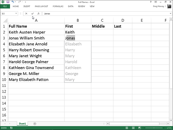
Figure 2-13: Data Table containing full names that need to be split up in separate columns using Flash Fill.

Rather than manually enter the first, middle, or last names in the respective columns (or attempt to copy the entire client name from column A and then edit out the parts not needed in First Name, Middle Name, and Last Name columns), you can use Flash Fill to quickly and effectively do the job. And here’s how you do it:

1. Type Keith in cell B2 and complete the entry with the or Enter key.

When you complete this entry with the down arrow key or Enter key on your keyboard, Excel moves the cell pointer to cell B3 where you only have to type the first letter of the next name for Flash Fill to get the picture.

2. In Cell B3, only type J, the first letter of the second client’s first name.

Flash Fill immediately does an AutoFill-type maneuver by suggesting the rest of the second client’s first name, Jonas, as the text to enter in this cell. At the same time, Flash Fill suggests entering all the remaining first names from the full names in column A in column B (see Figure 2-13).

3. Complete the entry of Jonas in cell B3 by pressing the Enter key or an arrow key.

The moment you complete the data entry in cell B3, the First Name column’s done: Excel enters all the other first names in column B at the same time!

To complete this example name table by entering the middle and last names in columns C and D, respectively, you simply repeat these steps in those columns. You enter the first middle name, Austen, from cell A2 in cell C2 and then type W in cell C3. Complete the entry in cell C3 and the middle name entries in that column are done. Likewise, you enter the first last name, Harper, from cell A2 in cell D2 and then type S in cell D3. Complete the entry in cell D3, and the last name entries for column D are done, completing the entire data table.

By my count, completing the data entry in this Client Name table required me to make a total of 26 keystrokes, 20 of which were for typing in the first, middle, and last name of the first client along with the initial letters of the first, middle, and last name of the second client and the other six to complete these entries. If Column A of this Client Name table contains the full names of hundreds or even thousands of clients, these 26 keystrokes is insignificant compared to the number that would be required to manually enter their first, middle, and last names in its separate First Name, Middle Name, and Last Name columns or even to edit down copies of the full names in each of them.

Keep in mind that Flash Fill works perfectly at extracting parts of longer data entries in a column provided that all the entries follow the same pattern and use same type of separators (spaces, commas, dashes, and the like). For example, in Figure 2-13, there’s an anomaly in the full name entries in cell A9 where only the middle initial with a period is entered instead of the full middle. In this case, Flash Fill simply enters M in cell C9 and you have to manually edit its entry to add the necessary period. Also, remember that Flash Fill’s usefulness isn’t restricted to all-text entries as in my example Client Name table. It can also parse entries that mix text and numbers such as part numbers (AJ-1234, RW-8007, and so forth).

Inserting special symbols

Excel makes it easy to enter special symbols, such as foreign currency indicators, and special characters, such as the trademark and copyright symbols, into your cell entries. To add a special symbol or character to a cell entry you’re making or editing, select Insert⇒Symbol on the Ribbon or press Alt+NU to open the Symbol dialog box.

The Symbol dialog box contains two tabs: Symbols and Special Characters. To insert a mathematical or foreign currency symbol on the Symbols tab, select its symbol in the list box and then click the Insert button. (You can also do this by double-clicking or double-tapping the symbol.) To insert characters, such as foreign language or accented characters from other character sets, click the Subset drop-down button followed by the name of the set in the drop-down list and the desired characters in the list box. You can also insert commonly used currency and mathematical symbols, such as the pound or plus-or-minus symbol, by selecting them in the Recently Used Symbols section at the bottom of this tab.

To insert special characters, such as the registered trademark, paragraph symbol, and so forth, you click the Special Characters tab of the Symbol dialog box followed by the symbol in the scrolling list and the Insert button. (You can insert one of these special characters by double-clicking or double-tapping it also.)

When you finish inserting special symbols and characters, close the Symbol dialog box by pressing Esc or clicking the Close button in its upper-right corner.

Entries all around the block

When you want to enter a table of information in a new worksheet, you can simplify the job of entering the data if you select all the empty cells in which you want to make entries before you begin entering any information. Just position the cell pointer in the first cell of what is to become the data table and then select all the cells in the subsequent columns and rows. (For information on the ways to select a range of cells, see Chapter 3.) After you select the block of cells, you can begin entering the first entry.

When you select a block of cells (also known as a range) before you enter information, Excel restricts data entry to that range as follows:

The program automatically advances the cell pointer to the next cell in the range when you click the Enter button on the Formula bar or press the Enter key to complete each cell entry.

In a cell range that contains several different rows and columns, Excel advances the cell pointer down each row of the column while you make your entries. When the cell pointer reaches the cell in the last row of the column, the cell pointer advances to the first selected row in the next column to the right. If the cell range uses only one row, Excel advances the cell pointer from left to right across the row.

When you finish entering information in the last cell in the selected range, Excel positions the cell pointer in the first cell of the now-completed data table. To deselect the cell range, select a single cell in the worksheet (inside or outside the selected range — it doesn’t matter) or press one of the arrow keys.

Be sure that you don’t press one of the arrow keys to complete a cell entry within a preselected cell range instead of clicking the Enter button or pressing Enter. Pressing an arrow key deselects the range of cells when Excel moves the cell pointer. To move the cell pointer around a cell range without deselecting the range, try these methods:

Press Enter to advance to the next cell down each row and then across each column in the range. Press Shift+Enter to move up to the previous cell.

Press Tab to advance to the next cell in the column on the right and then down each row of the range. Press Shift+Tab to move left to the previous cell.

Press Ctrl+. (period) to move from one corner of the range to another.

Data entry express

You can save a lot of time and energy when you want the same entry (text, value, or formula) to appear in many cells of the worksheet; you can enter the information in all the cells in one operation. You first select the cell ranges to hold the information. (Excel lets you select more than one cell range for this kind of thing — see Chapter 3 for details.) Then you construct the entry on the Formula bar and press Ctrl+Enter to put the entry into all the selected ranges.

The key to making this operation a success on a physical keyboard is to hold the Ctrl key down while you press Enter so that Excel inserts the entry on the Formula bar into all the selected cells. If you forget to hold Ctrl and you just press Enter, Excel places the entry in the first cell only of the selected cell range. On the Windows virtual keyboard, you just tap Ctrl followed by Enter in succession.

You can also speed up data entry in a list that includes formulas by making sure that the Extend Data Range Formats and Formulas check box is selected in the Editing Options section of the Advanced tab in the Excel Options dialog box. (Choose File⇒Options⇒Advanced or press Alt+FTA.) When this check box is selected, Excel automatically formats new data that you type in the last row of a list to match that of like data in earlier rows and copies down formulas that appear in the preceding rows. Note, however, that for this new feature to kick in, you must manually enter the formulas and format the data entries in at least three rows preceding the new row.

How to Make Your Formulas Function Even Better

Earlier in this chapter, I show you how to create formulas that perform a series of simple mathematical operations, such as addition, subtraction, multiplication, and division. (See the section “Fabricating those fabulous formulas!”) Instead of creating complex formulas from scratch out of an intricate combination of these operations, you can find an Excel function to get the job done.

A function is a predefined formula that performs a particular type of computation. All you have to do to use a function is supply the values that the function uses when performing its calculations. (In the parlance of the Spreadsheet Guru, such values are the arguments of the function.) As with simple formulas, you can enter the arguments for most functions either as a numerical value (for example, 22 or –4.56) or, as is more common, as a cell reference (B10) or as a cell range (C3:F3).

Just as with a formula you build yourself, each function you use must start with an equal sign (=) so that Excel knows to enter the function as a formula rather than as text. Following the equal sign, you enter the name of the function (in uppercase or lowercase — it doesn’t matter, as long as you spell the name correctly). Following the name of the function, you enter the arguments required to perform the calculations. All function arguments are enclosed in a pair of parentheses.

If you type the function directly in a cell, remember not to insert spaces between the equal sign, function name, and the arguments enclosed in parentheses. Some functions use more than one value when performing their designated calculations. When this is the case, you separate each function with a comma (not a space).

After you type the equal sign and begin typing the first few letters of the name of the function you want to use, a drop-down list showing all the functions that begin with the letters you’ve typed appears immediately beneath the cell. When you see the name of the function you want to use on this list, double-click it and Excel finishes entering the function name in the cell and on the Formula bar as well as add the left parenthesis that marks the beginning of the arguments for the function.

Excel then displays all the arguments that the function takes beneath the cell, and you can indicate any cell or cell range that you want to use as the first argument by either pointing to it or typing its cell or range references. When the function uses more than one argument, you can point to the cells or cell ranges or enter the addresses for the second argument right after you enter a comma (,) to complete the first argument.

After you finish entering the last argument, you need to close off the function by typing a right parenthesis to mark the end of the argument list. The display of the function name along with its arguments that appeared beneath the cell when you first selected the function from the drop-down list then disappears. Click the Enter button or press Enter (or the appropriate arrow key) to then insert the function into the cell and have Excel calculate the answer.

Inserting a function into a formula with the Insert Function button

Although you can enter a function by typing it directly in a cell, Excel provides an Insert Function command button on the Formula bar you can use to select any of Excel’s functions. When you select this button, Excel opens the Insert Function dialog box (shown in Figure 2-14) where you can select the function you want to use. After you select your function, Excel opens the Function Arguments dialog box. In this dialog box, you can specify the function arguments. The real boon comes when you’re starting to use an unfamiliar function or one that’s kind of complex (some of these puppies can be hairy). You can get loads of help in completing the argument text boxes in the Function Arguments dialog box by clicking the Help on This Function link in the lower-left corner.

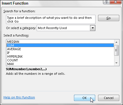
Figure 2-14: Select the function you want to use in the Insert Function dialog box.

The Insert Function dialog box contains three boxes: a Search for a Function text box, an Or Select a Category drop-down list box, and a Select a Function list box. When you open the Insert Function dialog box, Excel automatically selects Most Recently Used as the category in the Select a Category drop-down list box and displays the functions you usually use in the Select a Function list box.

If your function isn’t among the most recently used, you must then select the appropriate category of your function in the Select a Category drop-down list box. If you don’t know the category, you must search for the function by typing a description of its purpose in the Search for a Function text box and then press Enter or click the Go button. For example, to locate all the Excel functions that total values, you enter total in the Search for a Function list box and click the Go button. Excel then displays its list of recommended functions for calculating totals in the Select a Function list box. You can peruse the recommended functions by selecting each one. While you select each function in this list, the Insert Function dialog box shows you the required arguments followed by a description, at the bottom of the dialog box, of what the function does.

After you locate and select the function that you want to use, click the OK button to insert the function into the current cell and open the Function Arguments dialog box. This dialog box displays the required arguments for the function along with any that are optional. For example, suppose that you select the SUM function (the crown jewel of the Most Recently Used function category) in the Select a Function list box and then select OK. As soon as you do, the program inserts

SUM()

in the current cell and on the Formula bar (following the equal sign), and the Function Arguments dialog box showing the SUM arguments appears on the screen (as shown in Figure 2-15). This is where you add the arguments for the SUM function.

As shown in Figure 2-15, you can sum up to 255 numbers in the Function Arguments dialog box. What’s not obvious, however (there’s always some trick, huh?), is that these numbers don’t have to be in single cells. In fact, most of the time you’ll be selecting a whole slew of numbers in nearby cells (in a multiple cell selection — that range thing) that you want to total.

Figure 2-15: Specify the arguments to use in the selected function in the Function Arguments dialog box.

To select your first number argument in the dialog box, you select the cell (or block of cells) in the worksheet while the insertion point is in the Number1 text box. Excel then displays the cell address (or range address) in the Number1 text box while, at the same time, showing the value in the cell (or values, if you select a bunch of cells) in the box to the right. Excel displays the total near the bottom of the Function Arguments dialog box after the words Formula result=.

When selecting cells, you can minimize this arguments dialog box to just the contents of the Number1 text box by dragging the cell pointer through the cells to sum in the worksheet. After you minimize the arguments dialog box while selecting the cells for the first argument, you can then expand it again by releasing the mouse button.

You can also reduce the dialog box to the Number1 argument text box by clicking the Minimize Dialog Box button on the right of the text box, selecting the cells, and then clicking the Maximize Dialog Box button (the only button displayed on the far right) or by pressing the Esc key. Instead of minimizing the dialog box, you can also temporarily move it out of the way by clicking on any part and then dragging the dialog box to its new destination on the screen.

If you’re adding more than one cell (or a bunch of cells) in a worksheet, press the Tab key or click the Number2 text box to move the insertion point to that text box. (Excel responds by extending the argument list with a Number3 text box.) Here is where you specify the second cell (or cell range) to add to the one now showing in the Number1 text box. After you select the cell or second cell range, the program displays the cell address(es), the numbers in the cell(s) to the right, and the running total near the bottom of the Function Arguments dialog box after Formula result= (as shown in Figure 2-15). You can minimize the entire Function Arguments dialog box down to just the contents of the argument text box you’re dealing with (Number2, Number3, and so on) by clicking its particular Minimize Dialog Box button if the dialog box obscures the cells that you need to select.

When you finish pointing out the cells or bunch of cells to sum, click the OK button to close the Function Arguments dialog box and put the SUM function in the current cell.

Editing a function with the Insert Function button

You can also use the Insert Function button to edit formulas that contain functions right from the Formula bar. Select the cell with the formula and function to edit before you select the Insert Function button (the one sporting the fx that appears immediately in front of the current cell entry on the Formula bar).

As soon as you select the Insert Function button, Excel opens the Function Arguments dialog box where you can edit its arguments. To edit just the arguments of a function, select the cell references in the appropriate argument’s text box (marked Number1, Number2, Number3, and so on) and then make whatever changes are required to the cell addresses or select a new range of cells.

Excel automatically adds any cell or cell range that you highlight in the worksheet to the current argument. If you want to replace the current argument, you need to highlight it and remove its cell addresses by pressing the Delete key before you highlight the new cell or cell range to use as the argument. (Remember that you can always minimize this dialog box or move it to a new location if it obscures the cells you need to select.)

When you finish editing the function, press Enter or click the OK button in the Function Arguments dialog box to put it away and update the formula in the worksheet.

I’d be totally lost without AutoSum

Before leaving this fascinating discussion on entering functions, I want you to get to the AutoSum tool in the Editing group on the Home tab of the Ribbon. Look for the Greek sigma (Σ) symbol. This little tool is worth its weight in gold. In addition to entering the SUM, AVERAGE, COUNT, MAX, or MIN functions, it also selects the most likely range of cells in the current column or row that you want to use as the function’s argument and then automatically enters them as the function’s argument. Nine times out of ten, Excel selects (with the marquee or moving dotted line) the correct cell range to total, average, count, and so forth. For that tenth case, you can manually correct the range by simply dragging the cell pointer through the block of cells to sum.

Simply select the AutoSum button followed by Sum on the drop-down menu on the Home tab when you want to insert the SUM function into the current cell. The quicker method to select this function is to press Alt+= (the Alt key plus the equal to symbol on the top row).

If you want to use the AutoSum button to insert another function, such as AVERAGE, COUNT, MAX, or MIN, you need to click its drop-down button and select the name of the desired function on its pop-up menu (click Count Numbers on the menu to insert the COUNT function). If you select the More Functions command on this menu, Excel opens the Insert Function dialog box as though you had clicked the fx button on the Formula bar.

In Figure 2-16, check out how to use AutoSum to total the sales of Jack Sprat Diet Centers in row 3. Position the cell pointer in cell E3 where the first-quarter total is to appear and then select Sum on the AutoSum drop-down menu (or press Alt+=). Excel inserts SUM (equal sign and all) onto the Formula bar; places a marquee around the cells B3, C3, and D3; and uses the cell range B3:D3 as the argument of the SUM function.

Figure 2-16: To total Jack Sprat Diet Centers first quarter sales for row 3, click the AutoSum button in cell E3 and then click Enter.

Now look at the worksheet after you insert the function in cell E3 (see Figure 2-17). The calculated total appears in cell E3 while the following SUM function formula appears in the Formula bar:

=SUM(B3:D3)

After entering the function to total the sales of Jack Sprat Diet Centers, you can copy this formula to total sales for the rest of the companies by dragging the fill handle down column E until the cell range E3:E10 is highlighted (as shown in Figure 2-17).

Look at Figure 2-18 to see how you can use AutoSum to total the January sales for all the Mother Goose Enterprises in column B. Position the cell pointer in cell B10 where you want the total to appear. Select Sum on the AutoSum’s drop-down menu, and Excel places the marquee around cells B3 through B9 and correctly enters the cell range B3:B9 as the argument of the SUM function.

Figure 2-17: The worksheet with the first-quarter totals calculated with AutoSum.

Figure 2-18: Select AutoSum in cell B10 and click Enter to total the January sales for all companies in column B.

In Figure 2-19, you see the worksheet after inserting the function in cell B10 and using the AutoFill feature to copy the formula to cells C10 and D10 to the right. (To use AutoFill, drag the fill handle through the cells to the right until you reach cell D10. Release the mouse button or remove your finger or stylus from the touchscreen.)

Figure 2-19: The worksheet after copying the SUM function formulas using the fill handle.

Sums via Quick Analysis Totals

For those of you who don’t have the time or patience for adding totals to your worksheet tables with AutoSum and AutoFill, Excel 2013’s Totals feature of the new Quick Analysis tool is just the thing. The Quick Analysis tool offers a bevy of features for doing anything from adding conditional formatting (see Chapter 3), charts (see Chapter 10), pivot tables (see Chapter 9) and sparklines (see Chapter 10) to your worksheet tables. And it turns out Quick Analysis is also a whiz at adding running totals and sums to the rows and columns of your new worksheet tables.

To use the Quick Analysis tool, all you have to do is select the worksheet table’s cells (see Chapter 3 for details) and then click the Quick Analysis tool that automatically appears in the lower-right corner of the last selected cell. When you do, a palette of options (from Formatting to Sparklines) appears right beneath the tool.

To add totals to your selected table data, simply click the Totals button. You can then use your mouse or Touch Pointer to have Live Preview show you totals in a new row at the bottom by highlighting Running Total or in a new column on the right by highlighting Sum (shown in Figure 2-20). To actually add the SUM formulas with the totals to a new row or column, you simply click the Running Total or Sum button.

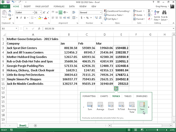
Figure 2-20: Using the Totals feature on the Quick Analysis tool to add a column of quarterly totals to a selected worksheet table.

To add the running totals to the sample worksheet table shown in Figure 2-20 after adding a column of quarterly totals with the Sum button, you simply select the table of data, A2 through D12 (to include the new Sum column), and click the Quick Analysis tool followed by the Totals and Running Total buttons. Then, edit the heading, Sum, in cell E2 to make it read Qtr 1 and you’re all done!

If you have trouble selecting the Quick Analysis tool to open its palette for any reason, simply right-click the cell selection and click the Quick Analysis item on its context menu.

Making Sure That the Data Is Safe and Sound

All the work you do in any of the worksheets in your workbook is at risk until you save the workbook as a disk file, normally on your computer’s hard drive. Should you lose power or should your computer crash for any reason before you save the workbook, you’re out of luck. You have to re-create each keystroke — a painful task made all the worse because it’s so unnecessary. To avoid this unpleasantness altogether, adopt this motto: Save your work any time that you enter more information than you could possibly bear to lose.

To encourage frequent saving on your part, Excel even provides you with a Save button on the Quick Access toolbar (the one with the picture of a 3¹⁄₄” floppy disk, the very first on the toolbar). You don’t even have to take the time and trouble to choose the Save command from the File pull-down menu (opened by choosing File) or even press Ctrl+S; you can simply click this tool whenever you want to save new work on disk.

When you click the Save button, press Ctrl+S, or choose File⇒Save for the first time, Excel 2013 displays the Save As screen similar to the one shown in Figure 2-21. By default, Excel 2013 selects the Documents folder on your Windows Live SkyDrive as the place to save the new workbook.

Figure 2-21: The Save As screen that appears after you select the Save command to save a new workbook.

---

---

To save the file locally instead — on your computer’s hard drive or a virtual drive on your local area network — click the Computer button under Windows Live’s SkyDrive.

When you click Computer, the right pane of the Save As screen then displays a list of Recent Folders where you’ve recently saved Excel workbook files as well as any mapped network drives and your device’s local Documents folder and Desktop. When you select the folder in this list into which you want to save the new workbook, Excel opens the Save As dialog box with the current contents of this folder displayed.

If none of the folders listed in the Computer pane of the Save As screen are where you want to save the workbook, go ahead and click the Browse button to open the Save As dialog box with the default location for saving workbook files from which you can select the drive and folder where the new workbook should be stored.

After the folder into which you want to save your new workbook is selected in the Save As dialog box, you then need to replace the temporary document name (Book1, Book2, and so forth) with a more descriptive filename in the File Name text box, select a new file format in the Save As Type drop-down list box, and select a new drive and folder before you save the workbook as a disk file.

When you finish making changes in the Save As dialog box, click the Save button or press Enter to have Excel 2013 save your work. When Excel saves your workbook file, the program saves all the information in every worksheet in your workbook (including the last position of the cell cursor) in the designated folder and drive.

You don’t have to fool with the Save As dialog box again unless you want to rename the workbook or save a copy of it in a different folder. If you want to do these things, you must choose File⇒Save As or press Alt+FA to choose the Save As command rather than clicking the Save button on the Quick Access toolbar or pressing Ctrl+S.

Changing the default file location

Whenever you open the Save As dialog box to save a new workbook file, Excel 2013 automatically selects the folder listed in the Default File Location text box on the Save tab of the Excel Options dialog box (File⇒Options⇒Save or Alt+FTS).

When you first start using Excel, the default folder is the Documents folder under your user name on your hard drive. For example, the directory path of the default folder where Excel 2013 automatically saves new workbook files on my computer is

C:UsersGregDocuments

The very generic Documents folder may not be the place on your hard drive where you want all the new workbooks you create automatically saved. To change the default file location to another folder on your computer, follow these steps:

1. Choose File⇒Options⇒Save or press Alt+FTS to open the Save tab of the Excel Options dialog box.

The Default File Location text box displays the directory path to the current default folder.

2. Click in the Default File Location text box.

To edit part of the path (such as the Documents folder name after your user name), insert the mouse pointer at that place in the path to set the insertion point.

3. Edit the existing path or replace it with the path to another folder in which you want all future workbooks to save to automatically.

4. Click OK to close the Excel Options dialog box.

The difference between the XLSX and XLS file format

Excel 2013 supports the use of the XML-based file format first introduced in Excel 2007 (which Microsoft officially calls the Microsoft Office Open XML format). This default file format is touted as being more efficient in saving data, resulting in smaller file size and offering superior integration with external data sources (especially when these resources are web-based ones supporting XML files). This XML-based file format carries the filename extension .xlsx and is the file format in which Excel automatically saves any new workbook you create.

The only problem with this newfangled XML-based file format is that it can’t be opened by earlier Excel versions (before Excel 2007). Therefore, if someone who needs to work with the workbook you’ve just created isn’t using Excel 2007 or hasn’t yet upgraded to Excel 2013, you need to save the new workbook in the earlier file format used in Excel versions 97 through 2003 with the old .xls filename extension. To do this, click the Save As Type drop-down button in the Save As dialog box and then click Excel 97-2003 Workbook (*.xls) in the drop-down menu.

Filename extensions, such as .xlsx and .xls, do not appear as part of the filename (even though they are appended) in the File Name text box in the Excel Save As dialog box unless you’ve specifically changed Windows’ folder options to show them. To make this change, open the Folder Options dialog box in Windows Explorer and then deselect the Hide Extensions for Known File Types check box on the View tab. To open the Folder Options dialog box in Windows 7 Explorer, click the Organize button and then select Folder and Search Options on its drop-down menu. To open this dialog box in Windows 8 Explorer, you select the View tab followed by the Options button on the Windows Explorer Ribbon.

Excel 2013 also supports a special binary file format called Excel Binary Workbook that carries the .xlsb filename extension. Select this binary format for huge spreadsheets that you create that have to be compatible with earlier versions of Excel.

Saving the Workbook as a PDF File

The PDF (Portable Document File) file format developed by Adobe Systems Incorporated enables people to open up and print documents without access to the original programs with which the documents were created.

Excel 2013 enables you to save your workbook files directly in this special PDF file format. You can readily share your Excel 2013 workbooks with users who don’t have Excel installed on their computers by saving them as PDF files. All they need to open and print the PDF copy of the workbook file is the free Adobe Reader software (which they can download from the Adobe Web site at www.adobe.com).

To save your workbook as a PDF file, you simply select the PDF option on the Save as Type drop-down list in the Save As dialog box. Excel then adds PDF-specific options to the bottom of the Save As dialog box, with the Standard (Publishing Online and Printing) button under the Optimize For heading and the Open File after Publishing check box selected.

If you want to make the resulting PDF file as small as possible (because your worksheet is so large), click the Minimum Size (Publishing Online) button under the Optimize For heading. If you want to change which parts of the workbook are saved in the resulting PDF (Excel automatically saves all ranges in the active worksheet of the workbook), click the Options button directly beneath the Minimum Size (Publishing Online) option and make the appropriate changes in the Options dialog box before you click OK.

If you don’t need to edit the filename (Excel automatically appends .pdf to the current filename) or the folder location in the Save As dialog box, simply click the Save button. Excel then saves a copy of the workbook in a PDF file format and, provided you don’t deselect the Open File after Publishing check box, automatically opens the workbook for your inspection in Adobe Reader. After viewing the PDF version in Adobe Reader, you can then return to your worksheet in Excel by clicking the Reader’s Close button (or pressing Alt+F4).

If you create an Excel 2013 workbook that incorporates new features not supported in earlier versions of Excel, instead of saving the workbook as an .xls file, thereby losing all of its 2010 enhancements, consider saving it as a PDF file. That way, co-workers still using pre-2010 Excel versions can still access the data in all its glory via Adobe Reader.

Document Recovery to the Rescue

Excel 2013 offers a document recovery feature that can help you in the event of a computer crash because of a power failure or some sort of operating system freeze or shutdown. The AutoRecover feature saves your workbooks at regular intervals. In the event of a computer crash, Excel displays a Document Recovery task pane the next time you start Excel after rebooting the computer.

When you first start using Excel 2013, the AutoRecover feature is set to automatically save changes to your workbook (provided that the file has already been saved) every ten minutes. You can shorten or lengthen this interval as you see fit. Choose File⇒Options⇒Save or press Alt+FTS to open the Excel Options dialog box with the Save tab selected. Use the spinner buttons or enter a new automatic save interval into the text box marked Save AutoRecover Information Every 10 Minutes before clicking OK.

After re-launching Excel 2013 after a computer crash that prevents you from saving your workbook file, the program opens with the Document Recovery task pane on the left side of the screen. This Document Recovery task pane shows the available versions of the workbook files that were open at the time of the computer crash. The original version of the workbook file is identified, including when it was saved, as is the recovered version of the file (displaying an .xlsb file extension) and when it was saved.

To open the recovered version of a workbook (to see how much of the work it contains that was unsaved at the time of the crash), position the mouse pointer over the AutoRecover version, click its drop-down menu button followed by Open. After you open the recovered version, you can then (if you choose) save its changes by selecting the Save button on the Quick Access toolbar or by choosing File⇒Save.

To save the recovered version of a workbook without bothering to first open it, click the recovered version’s drop-down button in the Document Recovery task pane, and then choose Save As. To abandon the recovered version permanently (leaving you with only the data in the original version), click the Close button at the bottom of the Document Recovery task pane. When you do this, an alert dialog box appears, giving you the chance to retain the recovered versions of the file for later viewing. To retain the files for later viewing, select the Yes (I Want to View These Files Later) radio button before clicking OK. To retain only the original versions of the files shown in the task pane, select the No (Remove These Files. I Have Saved the Files I Need) radio button instead.

The AutoRecover feature only works on Excel workbooks that you’ve saved at least one time (as explained in the earlier section “Making Sure That the Data Is Safe and Sound”). In other words, if you build a new workbook and don’t bother to save and rename it prior to experiencing a computer crash, the AutoRecover feature will not bring back any part of it. For this reason, it is very important that you get into the habit of saving new workbooks with the Save button on the Quick Access toolbar very shortly after beginning to work on its worksheets. Or use the trusty keyboard shortcut Ctrl+S.