Chapter 8

Doing What-If Analysis

In This Chapter

Performing what-if analysis with one- and two-variable data tables

Performing what-if analysis with goal seeking

Looking at different cases with the Scenario Manager

It would be a big mistake to regard Excel 2013 as merely a fancy calculator that shines at performing static computations, for the program excels (if you don’t mind the pun) at performing various types of more dynamic what-if analysis as well. What-if analysis enables you to explore the possibilities in a worksheet by inputting a variety of promising or probable values into the same equation and letting you see the possible outcomes in black and white (or, at least, in the cells of the spreadsheet).

In Excel 2013, what-if analysis comes in a wide variety of flavors (some of which are more involved than others). In this chapter, I introduce you to these three simple and straightforward methods:

Data tables enable you to see how changing one or two variables affect the bottom line (for example, you may want to know what happens to the net profit if you fall into a 25 percent tax bracket, a 35 percent tax bracket, and so on).

Goal seeking enables you to find out what it takes to reach a predetermined objective, such as how much you have to sell to make a $15 million profit this year.

Scenarios let you set up and test a wide variety of cases, all the way from the best-case scenario (profits grow by 8.5 percent) to the worst-case scenario (you don’t make any profit and actually lose money).

Playing What-If with Data Tables

Data tables enable you to enter a series of possible values that Excel then plugs into a single formula. Excel supports two types of data tables: a one-variable data table that substitutes a series of possible values for a single input value in a formula and a two-variable data table that substitutes series of possible values for two input values in a single formula.

Both types of data tables use the very same Data Table dialog box that you open by clicking Data⇒What-If Analysis⇒Data Table on the Ribbon or pressing Alt+AWT. The Data Table dialog box contains two text boxes: Row Input Cell and Column Input Cell.

When creating a one-variable data table, you designate one cell in the worksheet that serves either as the Row Input Cell (if you’ve entered the series of possible values across columns of a single row) or as the Column Input Cell (if you’ve entered the series of possible values down the rows of a single column).

When creating a two-variable data table, you designate two cells in the worksheet and, therefore, use both text boxes. One cell serves as the Row Input Cell that substitutes the series of possible values you’ve entered across columns of a single row, and the other cell serves as the Column Input Cell that substitutes the series of possible values you’ve entered down the rows of a single column.

Creating a one-variable data table

Figure 8-1 shows a 2014 sales projections spreadsheet for which a one-variable data table is to be created. In this worksheet, the projected sales amount in cell B5 is calculated by adding last year’s sales total in cell B2 to the amount that we expect it to grow in 2014 (calculated by multiplying last year’s total in cell B2 by the growth percentage in cell B3), giving you the formula

=B2+(B2*B3)

Because I clicked the Create From Selection command button on the Ribbon’s Formulas tab after making A2:B5 the selection and accepted the Left Column check box default, the formula uses the row headings in column A and reads:

=Sales_2013+(Sales_2013*Growth_2014)

Figure 8-1: Sales projection spreadsheet with a column of possible growth percentages to plug into a one-variable data table.

As you can see in Figure 8-2, I entered a column of possible growth rates ranging from 1% all the way to 5.5% down column B in the range B8:B17. To create the one-variable data table shown in Figure 8-2 that plugs each of these values into the sales growth formula, I follow these simple steps:

1. Copy the original formula entered in cell B5 into cell C7 by typing = (equal to) and then clicking cell B5 to create the formula =Projected_Sales_2014.

The copy of the original formula (to substitute the series of different growth rates in B8:B17 into) is now the column heading for the one-variable data table.

2. Select the cell range B7:C17.

The range of the data table includes the formula along with the various growth rates.

3. Click Data⇒What-If Analysis⇒Data Table on the Ribbon.

Excel opens the Data Table dialog box.

4. Click the Column Input Cell text box in the Data Table dialog box and then click cell B3, the Growth_2014 cell with the original percentage, in the worksheet.

Excel inserts the absolute cell address, $B$3, into the Column Input Cell text box.

Figure 8-2: Sales projection spreadsheet after creating the one-variable data table in the range C8:C17.

5. Click OK to close the Data Table dialog box.

As soon as you click OK, Excel creates the data table in the range C8:C17 by entering a formula using its TABLE function into this range. Each copy of this formula in the data table uses the growth rate percentage in the same row in column B to determine the possible outcome.

6. Click cell C7, then click the Format Painter command button in the Clipboard group on the Home tab and drag through the cell range C8:C17.

Excel copies the Accounting number format to the range of possible outcomes calculated by this data table.

A couple of important things to note about the one-variable data table created in this spreadsheet:

If you modify any growth-rate percentages in the cell range B8:B17, Excel immediately updates the associated projected sales result in the data table. To prevent Excel from updating the data table until you click the Calculate Now (F9) or Calculate Sheet command button (Shift+F9) on the Formulas tab, click the Calculation Options button on the Formulas tab and then click the Automatic Except for Data Tables option (Alt+MXE).

If you try to delete any single TABLE formula in the cell range C8:C17, Excel displays a Cannot Change Part of a Data Table alert. You must select the entire range of formulas (C8:C17 in this case) before you press Delete or click the Clear or Delete button on the Home tab.

---

---

Creating a two-variable data table

To create a two-variable data table, you enter two ranges of possible input values for the same formula in the Data Table dialog box: a range of values for the Row Input Cell across the first row of the table and a range of values for the Column Input Cell down the first column of the table. You then enter the formula (or a copy of it) in the cell located at the intersection of this row and column of input values.

Figure 8-3 illustrates this type of situation. This version of the projected sales spreadsheet uses two variables to calculate the projected sales for year 2014: a growth rate as a percentage of increase over last year’s sales (in cell B3 named Growth_2014) and expenses calculated as a percentage of last year’s sales (in cell B4 named Expenses_2014). In this example, the original formula created in cell B5 is a bit more complex:

=Sales_2013+(Sales_2013*Growth_2014) - (Sales_2013*Expenses_2014)

To set up the two-variable data table, I added a row of possible Expenses_2014 percentages in the range C7:F7 to a column of possible Growth_2014 percentages in the range B8:B17. I then copied the original formula named Projected_Sales_2014 from cell B5 to cell B7, the cell at the intersection of this row of Expenses_2014 percentages and column of Growth_2014 percentages with the formula:

=Projected_Sales_2014

Figure 8-3:Sales projection spreadsheet with a series of possible growth and expense percentages to plug in to a two-variable data table.

With these few steps, I created the two-variable data table you see in Figure 8-4:

1. Select the cell range B7:F17.

This cell range incorporates the copy of the original formula along with the row of possible expenses and growth-rate percentages.

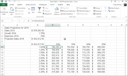
Figure 8-4: Sales projection spreadsheet after creating the two-variable data table in the range C8:F17.

2. Click Data⇒What-If Analysis⇒Data Table on the Ribbon.

Excel opens the Data Table dialog box with the insertion point in the Row Input Cell text box.

3. Click cell B4 to enter the absolute cell address, $B$4, in the Row Input Cell text box.

4. Click the Column Input Cell text box and then click cell B3 to enter the absolute cell address, $B$3, in this text box.

5. Click OK to close the Data Table dialog box.

Excel fills the blank cells of the data table with a TABLE formula using B4 as the Row Input Cell and B3 as the Column Input Cell.

6. Click cell B7, then click the Format Painter command button in the Clipboard group on the Home tab and drag through the cell range C8:F17 to copy the Accounting number format with no decimal places to this range.

This Accounting number format is too long to display given the current width of columns C through F — indicated by the ###### symbols. With the range C8:F17 still selected from using the Format Painter, Step 7 fixes this problem.

7. Click the Format command button in the Cells group of the Home tab and then click AutoFit Column Width on its drop-down menu.

The array formula {=TABLE(B4,B3)} that Excel creates for the two-variable data table in this example specifies both a Row Input Cell argument (B4) and a Column Input Cell argument (B3). (See the nearby “Array formulas and the TABLE function in data tables” sidebar.) Because this single array formula is entered into the entire data table range of C8:F17, any editing (in terms of moving or deleting) is restricted to this range.

Playing What-If with Goal Seeking

Sometimes when doing what-if analysis, you have a particular outcome in mind, such as a target sales amount or growth percentage. When you need to do this type of analysis, you use Excel’s Goal Seek feature to find the input values needed to achieve the desired goal.

To use the Goal Seek feature located on the What-If Analysis button’s drop-down menu, you need to select the cell containing the formula that will return the result you’re seeking (referred to as the set cell in the Goal Seek dialog box). Then indicate the target value you want the formula to return as well as the location of the input value that Excel can change to reach this target.

Figures 8-5 and 8-6 illustrate how you can use the Goal Seek feature to find out how much sales must increase to realize first quarter net income of $225,000 (given certain growth, cost of goods sold, and expense assumptions) in a sales forecast table.

Figure 8-5: Use goal seeking to find out how much sales must increase to reach a target income.

Figure 8-6: Forecast spreadsheet showing goal-seeking solution.

To find out how much sales must increase to return a net income of $225,000 in the first quarter, select cell B7, which contains the formula that calculates the forecast for the first quarter of 2014 before you click Data⇒What-If Analysis⇒Goal Seek on the Ribbon or press Alt+AWG.

This action opens the Goal Seek dialog box, similar to the one shown in Figure 8-5. Because cell B7 is the active cell when you open this dialog box, the Set Cell text box already contains the cell reference B7. You then click in the To Value text box and enter 225000 as the goal. Then, you click the By Changing Cell text box and click cell B3 in the worksheet (the cell that contains the first quarter sales) to enter the absolute cell address, $B$3, in this text box.

Figure 8-6 shows you the Goal Seek Status dialog box that appears when you click OK in the Goal Seek dialog box to have Excel go ahead and adjust the sales figure to reach your desired income figure. As this figure shows, Excel increases the sales in cell B3 from $250,000 to $432,692.31 which, in turn, returns $225,000 as the income in cell B7.

The Goal Seek Status dialog box informs you that goal seeking has found a solution and that the current value and target value are now the same. When this is not the case, the Step and Pause buttons in the dialog box become active, and you can have Excel perform further iterations to try to narrow and ultimately eliminate the gap between the target and current value.

If you want to keep the values entered in the worksheet as a result of goal seeking, click OK to close the Goal Seek Status dialog box. If you want to return to the original values, click the Cancel button instead.

To flip between the “after” and “before” values when you’ve closed the Goal Seek Status dialog box, click the Undo button or press Ctrl+Z to display the original values before goal seeking and click the Redo button or press Ctrl+Y to display the values engendered by the goal seeking solution.

Making the Case with Scenario Manager

Excel’s Scenario Manager option on the What-If Analysis button’s drop-down menu on the Data tab of the Ribbon enables you to create and save sets of different input values that produce different calculated results, named scenarios (such as Best Case, Worst Case, and Most Likely Case). Because these scenarios are saved as part of the workbook, you can use their values to play what-if simply by opening the Scenario Manager and having Excel show the scenario in the worksheet.

After setting up the various scenarios for a spreadsheet, you can also have Excel create a summary report that shows both the input values used in each scenario as well as the results they produce in your formula.

Setting up the various scenarios

The key to creating the various scenarios for a table is to identify the various cells in the data whose values can vary in each scenario. You then select these cells (known as changing cells) in the worksheet before you open the Scenario Manager dialog box by clicking Data⇒What-If Analysis⇒Scenario Manager on the Ribbon or by pressing Alt+AWS.

Figure 8-7 shows the Sales Forecast 2014 table after selecting the three changing cells in the worksheet — H3 named Sales_Growth, H4 named COGS (Cost of Goods Sold), and H6 named Expenses — and then opening the Scenario Manager dialog box (Alt+AWS).

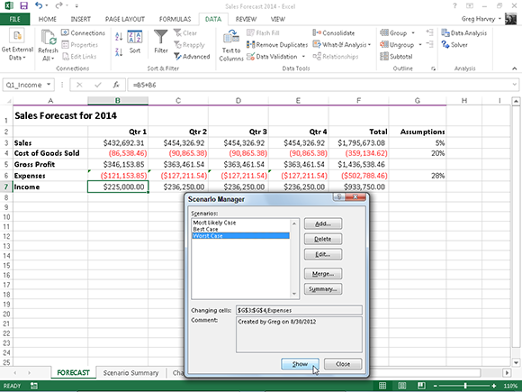
Figure 8-7: Add various scenarios to the Sales Forecast 2014 table.

I want to create three scenarios using the following sets of values for the three changing cells:

Most Likely Case where the Sales_Growth percentage is 5%, COGS is 20%, and Expenses is 28%

Best Case where the Sales_Growth percentage is 8%, COGS is 18%, and Expenses is 20%

Worst Case where the Sales_Growth percentage is 2%, COGS is 25%, and Expenses is 35%

To create the first scenario, I click the Add button in the Scenario Manager dialog box to open the Add Scenario dialog box, enter Most Likely Case in the Scenario Name box, and then click OK. (Remember that the three cells currently selected in the worksheet, H3, H4, and H6, are already listed in the Changing Cells text box of this dialog box.)

Excel then displays the Scenario Values dialog box where I accept the following values already entered in each of the three text boxes (from the Sales Forecast 2014 table), Sales_Growth, COGS, and Expenses, before clicking its Add button:

0.05 in the Sales_Growth text box

0.2 in COGS text box

0.28 in the Expenses text box

Always assign range names as described in Chapter 6 to your changing cells before you begin creating the various scenarios that use them. That way, Excel always displays the cells’ range names rather than their addresses in the Scenario Values dialog box.

After clicking the Add button, Excel redisplays the Add Scenario dialog box where I enter Best Case in the Scenario Name box and the following values in the Scenario Values dialog box:

0.08 in the Sales_Growth text box

0.18 in the COGS text box

0.20 in the Expenses text box

After making these changes, I click the Add button again. Doing this opens the Add Scenario dialog box where I enter Worst Case as the scenario name and the following scenario values:

0.02 in the Sales_Growth text box

0.25 in the COGS text box

0.35 in the Expenses text box

Because this is the last scenario that I want to add, I then click the OK button instead of Add. Doing this opens the Scenario Manager dialog box again, this time displaying the names of all three scenarios — Most Likely Case, Best Case, and Worst Case — in its Scenarios list box. To have Excel plug the changing values assigned to any of these three scenarios into the Sales Forecast 2014 table, I click the scenario name in this list box followed by the Show button.

After adding the various scenarios for a table in your spreadsheet, don’t forget to save the workbook after closing the Scenario Manager dialog box. That way, you’ll have access to the various scenarios each time you open the workbook in Excel simply by opening the Scenario Manager, selecting the scenario name, and clicking the Show button.

Producing a summary report

After adding your scenarios to a table in a spreadsheet, you can have Excel produce a summary report like the one shown in Figure 8-8. This report displays the changing and resulting values for not only all the scenarios you’ve defined, but also the current values that are entered into the changing cells in the worksheet table at the time you generate the report.

To produce a summary report, open the Scenario Manager dialog box (Data⇒What-If Analysis⇒Scenario Manager or Alt+AWS) and then click the Summary button to open the Scenario Summary dialog box.

This dialog box gives you a choice between creating a (static) Scenario Summary (the default) and a (dynamic) Scenario PivotTable Report (see Chapter 9). You can also modify the range of cells in the table that is included in the Result Cells section of the summary report by adjusting the cell range in the Result Cells text box before you click OK to generate the report.

After you click OK, Excel creates the summary report for the changing values in all the scenarios (and the current worksheet) along with the calculated values in the Result Cells on a new worksheet (named Scenario Summary). You can then rename and reposition the Scenario Summary worksheet before you save it as part of the workbook file.

Figure 8-8: Scenario Summary report showing the various scenarios added to the Sales Forecast 2014 table.

---

---