
Chapter 9
Some Constructions of Cross-Over Designs
9.1 INTRODUCTION
The construction and looking into the existence or nonexistence of designs is as important as providing the analysis for a given class of designs. Finite geometries, methods of differences, patchwork methods, and recursive methods are commonly used procedures for constructing designs. In Section 9.2, a brief review of Galois fields (GF) is provided, and in subsequent sections, some construction methods of the previously introduced designs are considered.
9.2 GALOIS FIELDS
Given a set of elements, F, a system ![]() is said to be a field, if the following conditions are satisfied:
is said to be a field, if the following conditions are satisfied:
- a, b ∈ F ⇒ a + b ∈ F, a · b ∈ F.
- a + (b + c) = (a + b) + c, a · (b · c) = (a · b) · c.
- a + b = b + a, a · b = b · a.
- ∃0, such that a + 0 = a, ∃1, such that a · 1 = a.
- ∃ (-a), such that a + (-a) = 0.
- ∀ a ≠ 0, ∃ (a– 1), such that a · (a- 1) = 1.
- a · (b + c) = a · b + a · c.
The number of elements, s, in a field is finite if s is a prime or prime power. These elements are called Galois fields and are written as GF(s). The quantity a is said to be congruent to b modulus s and is written a ≡ b(mod s), iff, a – b is divisible by s. If s is a prime p, the set of integers {0, 1, …, p - 1} is a field if these are multiplied or added in the usual manner and are reduced by mod p. For example, with s = 5, a field of 5 elements is {0, 1, 2, 3, 4}. Addition and multiplication of these elements are shown by the addition and multiplication tables given in Tables 9.2.1 and 9.2.2.
Table 9.2.1 Addition table with s = 5
| 0 | 1 | 2 | 3 | 4 | |
| 0 | 0 | 1 | 2 | 3 | 4 |
| 1 | 1 | 2 | 3 | 4 | 0 |
| 2 | 2 | 3 | 4 | 0 | 1 |
| 3 | 3 | 4 | 0 | 1 | 2 |
| 4 | 4 | 0 | 1 | 2 | 3 |
Table 9.2.2 Multiplication table with s = 5
| 0 | 1 | 2 | 3 | 4 | |
| 0 | 0 | 0 | 0 | 0 | 0 |
| 1 | 0 | 1 | 2 | 3 | 4 |
| 2 | 0 | 2 | 4 | 1 | 3 |
| 3 | 0 | 3 | 1 | 4 | 2 |
| 4 | 0 | 4 | 3 | 2 | 1 |
The entries in Tables 9.2.1 and 9.2.2 are, for example, 3 + 4 = 7 ≡ 2(mod 5) and 4 · 2 = 8 ≡ 3(mod 5). The entry in row 4, column 5 in Table 9.2.1 is 2, and the entry in row 5, column 3 is 3 in Table 9.2.2.
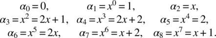
If s = pn, where n is a positive integer and p is a prime, the field elements are given as α0 = 0, α1, …, αs–1 where for multiplication purposes αi = xi–1 and for addition purposes ![]() , where ai’s are not all zero and belong to GF(p), and x is a primitive root satisfying an nth degree minimal function given in Table 9.2.3 that is equated to zero.
, where ai’s are not all zero and belong to GF(p), and x is a primitive root satisfying an nth degree minimal function given in Table 9.2.3 that is equated to zero.
Table 9.2.3 Some minimal functions
| GF | Minimal function |
| 22 | x 2 + x + 1 |
| 23 | x 3 + x2 + 1 |
| 24 | x 4 + x3 + 1 |
| 32 | x 2 + x + 2 |
| 33 | x 3 + 2x + 1 |
| 52 | x 2 + 2x + 3 |
The multiplicative and addition form of GF(32) are
9.3 Generalized Youden Designs
In Definition 5.6.4, a GYD was introduced. From that definition, it is clear that a GYD is an arrangement of v symbols in a k × b array such that
- Every symbol occurs m or m + 1 times in each row, as well as either n or n + 1 times in each column where m = ⌊b/v⌋ and n = ⌊k/v⌋.
- Every symbol occurs exactly r times.
- Every two distinct symbols occur together λ1 times in the same row and λ2 times in the same column.
Letting Lij to be a v × v Latin square for i = 1, 2, …, m and j = 1, 2, …, n, clearly, the following theorem holds:
Again,
9.4 Williams’ Balanced Residual Effects Designs
CODWR were first constructed systematically by Williams (1949) using one or two Latin squares depending on the number of treatments v is even or odd. In this section, construction methods of CODWR with k = v will be given.
Let M be a module of v elements. If ni is a k-component vector such that n′i = (ai1, ai2, …, aik), then denote by n′i,θ the column vector (ai1 + θ, ai2 + θ, …, aik + θ)′, where ai1, ai2, …, aik, θεM. The following theorem provides a method of constructing BRED, using the method of differences.
Specializing Theorem 9.4.1 to the cases of v even and odd with v = k, the following corollaries can be obtained.
Corollary 9.4.1.1 A BRED with parameters v = k = b, t = 1, λ = v, μ = v - 2, υ = 1 always exists when v is even.
Proof Let M = {0, 1, …, v - 1} and v = 2m. Further, let n′1 = {0, 2m - 1, 1, 2m - 2, …, m + 1, m - 1, m}. It is easy to verify that n1 satisfies all the requirements of Theorem 9.4.1, and the columns given by n′1,θ for θ = 0, 1, …, v - 1 provide the required design.
Corollary 9.4.1.2 A BRED with parameters v = k, b = 2v, t = 2, λ = 2v, μ = 2(v - 2), υ = 2 always exists when v is odd.
Proof Let v = 2m + 1 and M = {0, 1, …, v - 1}. Further, let n′1 = {0, 2m, 1, 2m - 1, …, m + 1, m} and n′2 = {m, m + 1, …, 2m - 1, 1, 2m, 0}. Then n1 and n2 satisfy the requirements of Theorem 9.4.1, and the columns given by n1,θ, n2,θ (θ = 0, 1, …, v - 1) provide the required design. Note that n2 is n1, written in reverse order.
It is interesting to see whether BREDs with v = k = b, t = 1, λ = v, μ = v - 2, υ = 1 exist for odd v. An exhaustive count shows that such BREDs do not exist for v = 3, 5, and 7. According to Hedayat and Afsarinejad (1978), the design for v = 9 as given in (9.4.1) was found by K.B. Mertz by using a computer, and the design for v = 15 as given in (9.4.2) was found by E. Sonneman by mimicking the design found by Mertz:


For v = 21, the design (9.4.3) was given by Hedayat and Afsarinejad (1975) based on the work of Mendelsohn (1968):

Hedayat and Afsarinejad (1978) gave the design for v = 27 as shown in (9.4.4) based on the work of Keedwell (1974):

9.5 Other Balanced Residual Effects Designs
The construction of BREDs with k < v, based on the work of Patterson (1952), will be discussed along with other miscellaneous constructions.
Balanced Arrays (or B-arrays) are widely used in factorial experiments, and a class of them can be used as BREDs. The definition of B-arrays is given as follows.
The idea of B-arrays was originally due to Rao (1946). A detailed treatment of orthogonal arrays can be found in Raghavarao (1971, Chapters 2 and 3).
If a B-array exists of strength 2 with λ-parameters satisfying
then the array can be used as a BRED. Such a BRED can be used in sequential experimentation, and the experiment can be terminated or continued at any period.
9.6 Combinatorially Overall Balanced Residual Effects Designs
Two series of COBREDs will be given in the following theorems.
9.7 Construction of Treatment Balanced Residual Effects Designs
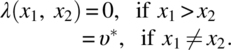
Following Section 8.5, we take ∞ to be the control treatment and 0, 1, …, v - 1 to be the active treatments. Let M be the module of v symbols, {0, 1, …, v - 1}. Let ∞ + θ = ∞, ∞ - θ = ∞, θ - ∞ = - ∞ for every θ ∈ M. Analogous to Theorem 9.4.1 for constructing BRED, we have Theorem 9.7.1.
As an example, let v = 3 active treatments and one control treatment ∞ and let a = 1. The three column vectors n′1 = (∞, 0, 1), n′2 = (0, ∞, 1), and n′3 = (0, 1, ∞) satisfy the requirements of Theorem 9.7.1, and the design is as follows:
| ∞ | ∞ | ∞ | 0 | 1 | 2 | 0 | 1 | 2 |
| 0 | 1 | 2 | ∞ | ∞ | ∞ | 1 | 2 | 0 |
| 1 | 2 | 0 | 1 | 2 | 0 | ∞ | ∞ | ∞ |
If there exists a BRED for v treatments in b units and k(<v) periods exist, then we can get a TBRED in k periods and bk subjects. We repeat the BRED k times and replace row i in the ith repetition by the control treatment ∞ for i = 1, 2, …, k. The parameters of this TBRED can easily be obtained. Using the columns n′1 = (0, 1, 6), n′2 = (0, 2, 5), and n′3 = (0, 4, 3) to get a BRED from Theorem 9.5.1, we can construct a TBRED for 7 active treatments and one control treatment ∞ in 3 periods and 63 units. The sets needed to get the design following Theorem 9.7.1 are (∞, 1, 6), (∞, 2, 5), (∞, 4, 3), (0,∞, 6), (0, ∞, 5), (0, ∞, 3), (0, 1, ∞), (0, 2, ∞), and (0, 4, ∞).
Given a BRED for v treatments in b units and k (<v) periods, we can get a TBRED in k + 1 periods. To construct the design, we replicate the BRED k times and add an extra period in each replication of the control treatment ∞. The extra period comes before the first period of BRED in the first replication and after the last period in the last replication. It is inserted between the (i - 1) and i periods of BRED in the ith replication for i = 2, 3, …, k - 1.
From the following BRED
for 3 treatments in 2 periods and 6 units, we get the TBRED
| ∞ | ∞ | ∞ | ∞ | ∞ | ∞ | 0 | 1 | 2 | 1 | 2 | 0 | 0 | 1 | 2 | 1 | 2 | 0 | ||||||||||
| 0 | 1 | 2 | 1 | 2 | 0 | ∞ | ∞ | ∞ | ∞ | ∞ | ∞ | 1 | 2 | 0 | 0 | 1 | 2 | ||||||||||
| 1 | 2 | 0 | 0 | 1 | 2 | 1 | 2 | 0 | 0 | 1 | 2 | ∞ | ∞ | ∞ | ∞ | ∞ | ∞ | ||||||||||
for 3 active and one control treatment in 3 periods on 18 units.
9.8 Some Construction of PBCOD (m)
We need to use PBCOD (m), when the number of treatments is very large and it is difficult to use many periods for experimentation.
If a PBIB design for v treatments in block size k exists, we can get a PBCOD (m) for v treatments by forming BRED for the treatments in each block of the PBIB design.
If v = n(n - 1)/2, the treatments can be arranged in a n × n array with empty diagonal and writing the v treatments above the diagonal and symmetrically filling the bottom of the diagonal. The treatments θ and ϕ are first associates if they occur in the same row or column of the n × n array, otherwise, second associates. This is called triangular association scheme. For example, with 6 treatments, we arrange them in the array

and understand

and
Using the triangular association scheme, we get a PBCOD (2) by forming n BREDs using the symbols in each row of the n × n array.
If v = n2, we get L2 association scheme by writing the v symbols in a n × n array and defining (θ, ϕ) = 1 if θ, ϕ occur in the same row or column, otherwise, second associates. For v = 9, we form

and get PBCOD (2) by forming six BREDs using the symbols in each row and each column.
Given two arrays
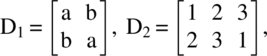
we define the symbolic Kronecker product of D1, D2, denoted by D1 ⊗ D2 as

For i = 1, 2, if Di is two BREDs or PBCOD (m) with vi treatments in ki periods with bi units, it can be verified that D1 ⊗ D2 is a BRED or PBCOD (m) for v1, v2 treatments in k1, k2 periods with b1, b2 units.
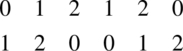
Let v = 2n and the treatments are arranged in a 2 × n array:
(1, 1) (1, 2) … (1, n).
(2, 1) (2, 2) … (2, n).
We form two BREDs Di with n treatments (i, 1), (i, 2), …, (i, n) for i = 1, 2. We add an extra period by putting (2, j) if the last period of D1 is (1, j) and (1, j) if the last period of D2 is (2, j) for j = 1, 2, …, n. The resulting design is PBCOD (m) with rectangular association scheme
9.9 Construction of Complete Set of Mols and Patterson’s Bred
We defined a complete set of MOLS in Section 5.11. In this section, we will discuss their construction method, and using them, we will give a construction method of Patterson’s BRED, whenever v is a prime or prime power.
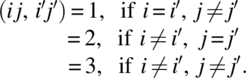
Let v be a prime or prime power, and let α0 = 0, α1, α2, ..., αv–1 be the elements of GF(v). It is known that the v - 1 arrays Li of v × v dimensionality whose (j, j′) cell is filled by ![]() provide a complete set of MOLS of order v (see Raghavarao, 1971, Chapter 1). If we call the columns of Li to be ℓi0, ℓi1, ℓi2, …, ℓi(v-1), the columns of Li+1 are ℓi0, ℓi2, ℓi3, …, ℓi(v–1), ℓi1.
provide a complete set of MOLS of order v (see Raghavarao, 1971, Chapter 1). If we call the columns of Li to be ℓi0, ℓi1, ℓi2, …, ℓi(v-1), the columns of Li+1 are ℓi0, ℓi2, ℓi3, …, ℓi(v–1), ℓi1.
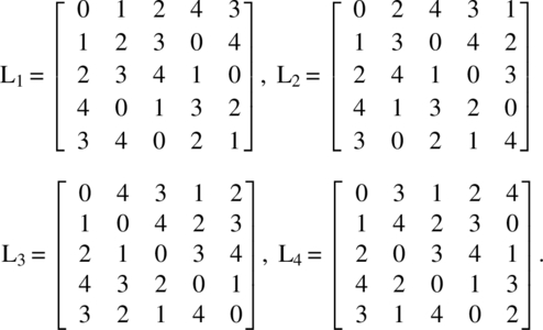
For example, let v = 5, and consider the elements of GF(5) given by α0 = 0, α1 = 1, α2 = 2, α3 = 4, α4 = 3.
The 4 MOLS of order 5 are
To construct BREDs of Patterson, interchange the rows and columns of a complete set of MOLS, and write them side by side to form a v × v(v - 1) array and take the first k rows to form BRED, for required k. To get a BRED for five treatments in three periods, we use the first three rows of the following array:
| BRED | 0 | 1 | 2 | 4 | 3 | 0 | 1 | 2 | 4 | 3 | 0 | 1 | 2 | 4 | 3 | 0 | 1 | 2 | 4 | 3 |
| 1 | 2 | 3 | 0 | 4 | 2 | 3 | 4 | 1 | 0 | 4 | 0 | 1 | 3 | 2 | 3 | 4 | 0 | 2 | 1 | |
| 2 | 3 | 4 | 1 | 0 | 4 | 0 | 1 | 3 | 2 | 3 | 4 | 0 | 2 | 1 | 1 | 2 | 3 | 0 | 4 | |
| 4 | 0 | 1 | 3 | 2 | 3 | 4 | 0 | 2 | 1 | 1 | 2 | 3 | 0 | 4 | 2 | 3 | 4 | 1 | 0 | |
| 3 | 4 | 0 | 2 | 1 | 1 | 2 | 3 | 0 | 4 | 2 | 3 | 4 | 1 | 0 | 4 | 0 | 1 | 3 | 2 |
9.10 Balanced Circular Arrangements
Given v, we arrange the v symbols in a circular form filling v(v - 1) positions such that every p symbols θ and ϕ occur next to each other once. Such arrangement always exists for any v, and we will discuss them in this section.
First, we assume v is even, say v = 2m, and we construct Williams’ BRED for 2m elements and wrap the columns in a circle without any repetition of a symbol and filling v(v - 1) positions. Proceed wrapping columns i, m + i for i = 1, 2, …, m ignoring repetitions to get the required design.
For v = 6, the BRED

gives the circular arrangement
For odd v = 2m + 1, we first prepare the circular arrangement in 2 m symbols and add (2m + 1)th symbol by replacing any 1 by {(2m + 1),1}, 2 by {(2m + 1), 2}, …, 2m by {(2m + 1),(2m)}.
From the circular arrangement given previously for v = 6, we get the arrangement for 7 symbols as follows:

If we want an arrangement where each treatment gives residual effect on itself, we can repeat each of the treatment i, for i = 1, 2, …, v in the circular arrangement in v(v–1) symbols.
9.11 CONCLUDING REMARKS
Some general construction methods of cross-over designs, discussed in the earlier chapter, were presented in this chapter. A catalogue of cross-over designs is given by Patterson and Lucas (1962). In practical situations, one may construct a suitable cross-over design, not necessarily a BRED or PBCOD (m), and analyze it. Recently, one of the authors has come across a situation in which a placebo (p) and two active treatments (A and B) were used as CODWR in a two sequence, five period design given by
P P
A P
P B
B P
P A
The analysis for such ad hoc designs can be easily constructed by the methods of Section 6.2.
The nonexistence of BREDs is not systematically studied. Isolated cases were discussed in Patterson (1952) and Pigeon and Raghavarao (1987).
There is a need to expand classes of PBCOD (m) by developing designs based on other association schemes. TBREDs were constructed by Pigeon (1984) following analogous methods discussed in Section 9.4. He gave a list of parameter sets whose solutions are unknown. The construction of those unsolved cases will present interesting venues for research in this area.
References
- Hedayat A, Afsarinejad K. In: Srivastava JN, editor. Repeated Measurements Designs I. A Survey of Statistical Designs and Linear Models. Amsterdam: North-Holland; 1975. p 229–242.
- Hedayat A, Afsarinejad K. Repeated measurements designs II. Ann Math Statist 1978;6:619–628.
- Keedwell AD. Some Problems Concerning Complete Latin Squares. Combinatorics (Proceedings of British Combinatorial Conference held in Aberystwyth in July 1973). Cambridge, UK: Cambridge University Press; 1974. p 89–96.
- Kiefer J. Balanced block designs and generalized Youden designs, 1. Construction (Patchwork). Ann Math Statist 1975;3:109–118.
- Mendelsohn NS. Hamilton decomposition of the complete directed n–graph. In: Erdos P, Katona G, editors. Theory of Graphs (Proceedings of Colloquium held at Tihany, Hungary in September 1966. Amsterdam: North Holland; 1968, p 237–241.
- Patterson HD. The construction of balanced designs for experiments involving sequences of treatments. Biometrika 1952;39:32–48.
- Patterson HD, Lucas HL. Change-over designs. Technical Bulletin No. 147, North Carolina Agricultural Experiment Station; 1962.
- Pigeon J. Residual effects designs for comparing treatments with a control. [Unpublished Ph.D. dissertation]. Philadelphia, PA: Temple University; 1984.
- Pigeon J, Raghavarao D. Crossover designs for comparing treatments with a control. Biometrika 1987;74:321–328.
- Raghavarao D. Construction and Combinatorial Problems in Design of Experiments. New York: Wiley; 1971.
- Rao CR. Hypercubes of strength “d” leading to confounded designs in factorial experiments. Bull Calcutta Math Soc 1946;38:67–78.
- Ruiz F, Seiden E. On construction of some families of generalized Youden designs. Ann Math Statist 1974;2:503–519.
- Seiden E, Wu CJ. A geometric construction of generalized Youden designs for v a power of a prime. Ann Math Statist 1978;6:452–460.
- Williams EJ. Experimental designs balanced for the estimation of residual effects of treatments. Aust J Sci Res 1949;2:149–168.
Further Reading
- Afsarinejad K. Repeated measurements designs – a review. Commun Statist—Theory Meth 1990;19:3985–4028.
- Afsarinejad K, Hedayat A. Repeated measurements designs for a model with self and carryover effects. J Statist Plan Inf 1978;106:449–459.
- Agrawal HL, Sharma RS. On trial and error method of construction of two-way designs. J Indian Statist Assoc 1972;10:9–16.
- Altan S, Raghavarao D. Nested Youden square designs. Biometrika 1996;83:242–245.
- Anderson TW. Repeated measures in auto-regressive processes. J Am Statist Assoc 1978;73:371–378.
- Atkinson GF. Designs for sequences of treatments with carry-over effects. Biometrics 1966;22:292–309.
- Bate S, Jones B. The construction of nearly balanced and nearly strongly balanced cross-over designs. J Statist Plan Inf 2006;136:3248–3267.
- Bate S, Jones B. A review of uniform cross-over designs. J Statist Plan Inf 2006;138:336–351.
- Bates DM, Watts DG, Nonlinear Regression Analysis and Its Applications. New York: Wiley; 1988.
- Beckman RJ, Nachtsheim CJ, Cook DR. Diagnostics for mixed-model analysis of variance. Technometrics 1987;29:413–426.
- Berchtold W. Analysis of a Cross-Over Experiment With ‘Proportion’ Numbers. Contributions to Applied Statistics. Birhaeuser Verlag; 1976.
- Berenblut II. Change-over designs with complete balance for first residual effects. Biometrics 1964;20:707–712.
- Berenblut II. The analysis of change-over designs with complete balance for first residual effects. Biometrics 1967;23:578–580.
- Berenblut II. Change-over designs balanced for the linear component of first residual effects. Biometrika 1968;55:297–303.
- Berenblut II. Treatment sequences balanced for the linear component of residual effects. Biometrics 1970;26:154–156.
- Bhapkar VP, Patterson KW. On some non-parametric tests for profile analysis of several multivariate samples. J Multivar Anal 1977;7:265–277.
- Bock RD. In: Harris CW, editor. Multivariate Analysis of Variance of Repeated Measurements. Problems in Measuring Change. Madison, WI: University of Wisconsin Press; 1963. p 85–103.
- Bradley JV. Complete counter balancing of immediate sequential effects in a Latin square design. J Am Statist Assoc 1958;53:525–528.
- Brandt AE. Tests of significance in reversal or switchback trials. Research Bulletin No. 234. Iowa Agricultural Experimental Station; 1938.
- Brayton RK, Coopersmith D, Hoffman AJ. Self orthogonal and Latin squares of all orders n ≠ 2, 3, 6. Bull Math Soc 1974;80:116–118.
- Brown H, Prescott R. Applied Mixed Models in Medicine. New York: John Wiley & Sons; 1999.
- Carriere K, Huang, R. Crossover designs for two-treatment clinical trials. J Statist Plan Inf 2000;87:125–134.
- Chassan JB. On the analysis of simple cross-overs with unequal number of replicates. Biometrics 1964;20:206–208.
- Cochran WG. Long-term agricultural experiments. J R Statist Soc 1939;6B:104–148.
- Cole JWL, Grizzle JE. Applications of multivariate analysis of variance to repeated measurements experiments. Biometrics 1966;22:810–828.
- Davidian M, Giltinan DM. Nonlinear Models for Repeated Measurement Data. London: Chapman & Hall; 1995.
- Davidson ML. Univariate versus multivariate tests in repeated measures experimental. Psychol Bull 1972;77:446–452.
- Denes J, Keedwell AD. Latin Squares and Their Applications. Budapest: Akademiai Kiado; 1974.
- Dette H, Pepelyshev A. Efficient experimental designs for sigmoidal growth models. J Statist Plan Inf 2008;138:2–17.
- Dey A, Balachandran G. A class of change-over designs balanced for first residual effect. J Indian Soc Agric Statist 1976;28:57–64.
- Dyke GV, Shelly CF. Serial designs balanced for effects of neighbours on both sides. J Agric Sci 1976;87:303–305.
- Enderlein G. Balanced changeover designs. Biom Zeit 1974;16:491–503.
- Federer WT, Atkinson GF. Tied-double-change-over designs. Biometrics 1964;20:168–181.
- Federer WT. The misunderstood split plot. In: Gupta, RP, editor. Applied Statistics. Amsterdam: North-Holland; 1975, p 9–39.
- Federer WT. Sampling, blocking, and model considerations for the r-row by c-column experiment designs. Biom Zeit 1976;18:595–607.
- Federer WT. Sampling, blocking, and model considerations for split plot and split block designs. Biom Zeit 1977;19:183–202.
- Federer WT, King F. Variations on Split Plot and Split Block Experiment Designs. New York: Wiley; 2007.
- Ferris GE. A modified Latin square design for taste testing. Food Res 1957;22:251–258.
- Finney DJ. Cross-over designs in bioassay. Proc R Soc 1956;145B:42–61.
- Finney DJ, Outhevaite AD. Serially balanced sequences in bio-assay. Proc R Soc 1956;145B:493–507.
- Freeman GH. Some experimental designs of use in changing from one set of treatments to another, Part 1. J R Statist Soc 1957;19B:154–162.
- Freeman GH. Families of designs for two successive experiments. Ann Math Statist 1958;29:1063–1078.
- Freeman GH. The use of the same experimental material for more than one set of treatments. Appl Statist 1959;8:13–20.
- Freeman GH. Experimental designs with unequal concurrences for estimating direct and remote effects of treatments. Biometrika 1973;60:559–563.
- Freeman GH. Row and column designs with two groups of treatments having different replications. J R Statist Soc 1975;37B:114–128.
- Geisser S. The Latin square as a repeated measurements design. Proceedings of the Fourth Berkley Smyposium; 20 June–30 July, 1960; Berkeley. Berkeley, CA: University of California Press, p 241–250.
- Gilbert EN. Latin squares which contain no repeated diagrams. SIAM Rev 1965;7:189–198.
- Gill JL, Magee WT. Balanced two-period cross-over designs for several treatments. J Anim Sci 1976;42:775–777.
- Gordon B. Sequence in groups with distinct partial product. Pac J Math 1961;11:1309–1313.
- Goswami RP. Efficiency of change-over design in animal experimentations. J Indian Soc Agric Statist 1970;22:43–56.
- Hedayat A. Some contributions to the theory of repeated measurement designs. Bull Inst Math Statist 1974;3:164.
- Hedayat A, Stufken J. Optimal and efficient crossover designs under different assumptions about carryover effects. J Biopharm Stat 2003;13:519–528.
- Hedayat A, Seiden E, Federer WT. Some families of designs for multistage experiments: mutually balanced Youden designs when the number of treatments is prime or twin primes. Ann Math Statist 1972;43:1517–1527.
- Hedayat A, Jacroux M, Majumdat D. Optimal designs for comparing test treatments with controls. Statist Sci 1988;4:462–476.
- Hedayat A, Zhong J, Nie L. Optimal and efficient designs for 2-parameter nonlinear models. J Statist Plan Inf 2004;124:205–217.
- Houston TP. Sequential counterbalancing in Latin squares. Ann Math Statist 1966;37:741–743.
- Huyhn H, Feldt LS. Conditions under which mean square ratios in repeated measurement designs have exact F distributions. J Am Statist Assoc 1970;65:1582–1589.
- Hwang FK. Constructions of some neighbor designs. Ann Statist 1973;1:786–790.
- Jones B, Deppe C. Recent developments in the design of cross-over trials: a brief review and bibliography. In: Altan S, Singh J, editors. Recent Advances in Experimental Designs and Related Topics. Huntington, NY: Nova Science Publishers; 2001. p 153–173.
- Keppel G. Design and Analysis: A Researcher’s Handbook. Englewood Cliffs, NJ: Prentice Hall Inc.; 1973.
- Khuri AI, Mukherjee B, Sinha BK, Ghosh, M. Design issues for generalized linear models: a review. Statist Sci 2006;21:376–399.
- Koch GG. Some aspects of the statistical analysis of ‘split plot’ experiments in completely randomized experiments. J Am Statist Assoc 1969;64:485–505.
- Koch GG. The use of non-parametric methods in the statistical analysis of a complex split plot experiment. Biometrics 1970;26:105–128.
- Koch GC, Landis JR, Freeman JL, Freeman Jr, DH, Lehnen RG. A general methodology of experiments with repeated measurement of categorical data. Biometrics 1977;33:133–159.
- Koch GG, Landis, JR, Freeman JL, Freeman Jr, DH, Lehnen RG. A general methodology for the analysis of experiments with repeated measurement of categorical data. Biometrics 1977;33:133–158.
- Kshirsagar AM. Recovery of inter-row and inter-column information in two-way designs. Ann Inst Statist Math 1971;23:263–278.
- Kshirsagar AM, Ranganathan S. Analysis of a class of two-way designs with recovery of inter-row and inter-column information. Calcutta Statist Assoc Bull 1968;17:15–24.
- Kshirsagar AM, Sinha PS, Analysis of a balanced incomplete two-way design. Ann Inst Statist Math 1968;20:469–476.
- Lawless JF. A note on certain types of BIBD balanced for residual effects. Ann Math Statist 1971;42:1439–1441.
- Lehnen RG, Koch GG. The analysis of categorical data from repeated measurement research designs. Polit Methodol 1974;1:103–123.
- Levin JR, Marascuilo LA. Post hoc analysis of repeated measures interactions and gain scores: whether the inconsistency? Psychol Bull 1977;84:247–248.
- Li G, Majumdar, D. D-optimal designs for logistic models with three and four parameters. J Statist Plan Inf 2008;138:1950–1959.
- Li G, Majumdar D. Some results on D-optimal designs for nonlinear models with applications. Biometrika 2009;96:487–493.
- Lin L. Assay validation using the concordance correlation coefficient. Biometrics 1992;48:599–604.
- Lucas HL. Bias in estimation of error in change-over trials with dairy cattle. J Agric Sci 1951;41:146.
- Magda CG. Circular balanced repeated measurement designs. Comm Statist—Theor Meth 1980;9A:1901–1918.
- Mason JM, Hinkelmann K. Change-over designs for testing different treatment factors at several levels. Biometrics 1971;27:430–435.
- Mielke Jr, PW. Squared rank test appropriate to weather modification cross-over design. Technometrics 1974;16:13–16.
- Monlezun CJ, Blouin DC, Malone LC. Contrasting split plot and repeated measures experiments and analysis. Am Statist 1984;38:21–27.
- Morrison DF. The optimal spacing of repeated measurements. Biometrics 1970;26:281–290.
- Morrison DF. The analysis of single sample of repeated measurements. Biometrics 1972;28:55–71.
- Muller KE, Stewart PW. Linear Model Theory: Univariate, Multivariate, and Mixed Models. New York: Wiley; 2006.
- Nair CR. Sequences balanced for pairs of residual effects. J Ann Statist Assoc 1967;62:205–225.
- Patterson HD. The analysis of change-over trials. J Agric Sci 1950;40:375–380.
- Patterson HD. Change-over trials. J R Statist Soc 1951;13B:256–271.
- Patterson HD. Non additivity in change-over designs for a quantitative factor at four levels. Biometrika 1970;57:537–549.
- Patterson HD. Quenouille’s change-over designs. Biometrics 1973;60:33–45.
- Patterson HD. Lucas HL. Extra-period change-over designs. Biometrics 1959;15:116–132.
- Pearce SC. Row-and-column designs. Appl Statist 1975;24:60–74.
- Poor DDS. Analysis of variance in repeated measures designs: two approaches. Psychol Bull 1973;80:204–209.
- Preece DA. Some row and column designs for two sets of treatments. Biometrics 1966;22:1–25.
- Preece DA. Balanced 6 × 6 designs for 9 treatments. Sankhya 1968;30B:443–446.
- Preece DA. Some new balanced row-and-column designs for two non-interacting sets of treatments. Biometrics 1971;27:426–430.
- Preece DA, Hall WB. Balanced designs for row-and-column experiment with two-non-interacting sets of treatments, one set being applied to all the rows. Aust J Statist 1975;17:186–191.
- Raghavarao D. A note on some balanced generalized two-way elimination of heterogeneity designs. J Indian Soc Agric Statist 1970;22:49–52.
- Raghavarao D. Cross-over designs in industry. In: Ghosh S, editor. Statistical Design and Analysis Industrial Experiment. New York: Marcel Dekker; 1990. p 517–530.
- Rao GN. A note on the methods of construction of some balanced generalized two-way elimination of heterogeneity designs. J Indian Soc Agric Statist 1973;25:143–150.
- Rao GN. Further contribution to balanced generalized two-way elimination of heterogeneity designs. Sankhya 1976;38B:72–79.
- Ratowsky D, Evans M, Alldredge J. Cross-Over Experiments. New York: Marcel Dekker; 1993.
- Rees DH. Some designs of use in serology. Biometrics 1967;23:779–791.
- Rees DH. Some observations on change-over trials. Biometrics 1969;25:413–417.
- Rouanet H, Lepine D. Comparison between treatments in a repeated measures design Anova and multivariate methods. Br J Math Statist Psychol 1970;23:147–163.
- Sampford MR. Methods of construction and analysis of serially balanced sequences. J R Statist Soc 1957;19B:286–304.
- Schaafsma W. Paired comparisons with order-effects. Ann Math Statist 1973;1:1027–1045.
- Scheehe PR, Bross DJ. Latin squares to balance immediate residual and other order effects. Biometrics 1961;17:405–414.
- Senn S. Cross-over trials in statistics in medicine: the first ‘25’ years. Stat Med 2006;25:3430–3442.
- Sharma VK. An easy method of constructing Latin square designs balanced for the immediate residual and other order effects. Canad J Statist 1975;3:119–124.
- Sharma VK. Change-over designs with complete balance for first and second residual effects. Canad J Statist 1977;5:121–132.
- Singh M, Dey A. Two-way elimination of heterogeneity. J R Statist Soc 1978;40B:58–63.
- Stufken J. Some families of optimal and efficient repeated measurements designs. J Statist Plan Inf 1991;27:75–83.
- Wallenstein S, Fisher AC. The analysis of two-period repeated measurements cross-over design with application to clinical trials. Biometrics 1977;33:261–272.
- Wang LL. A test for sequencing of a class of finite, groups with two generators. Am Math Soc Notices 1973;20:73T-A275 (Abstract).
- Weidman L. Serial arrays and change-over designs. Statist Plan Inf 1978;2:165–171.
- Williams EJ. Experimental designs balanced for pairs of residual effects. Aust J Sci Res 1950;3:351–363.
- Williams RM. Experimental designs for serially correlated observations. Biometrika 1952;39:151–167.
- Woodbury MA, Manton KG, Woodbury LA. An extension of the sign test for replicated measurements. Biometrics 1977;33:453–462.
- Wu SC, Williams JS, Mielke Jr, PW. Some designs and analyses for temporally independent experiments involving correlated bivariate responses. Biometrics 1972;28:1043–1061.
- Zimmermann H, Rahlfs V. Testing hypotheses in the two-period change-over with binary data. Biometrics 1978;20:133–141.