
Chapter 2
One-Sample Repeated Measurement Designs
2.1 INTRODUCTION
A random sample of N experimental units is selected, and on each unit, p responses are taken. The responses may all be taken at the same time or may be staggered over a period of different time intervals. It is also possible to treat each of the N homogeneous experimental units with the same treatment at the beginning of the experiment and take the data at different time intervals, to determine the effect or absorption of the treatment over a time interval. The jth response on the αth experimental unit will be represented by Yαj (j = 1, 2, …, p; α = 1, 2, …, N).
Let Y′α = (Yα1, Yα2, …, Yαp) be the p-dimensional response vector on the αth unit, and let Y = (Yαj) be the N × p data matrix of all responses on all experimental units.
We assume Yα ~ IMNp (μ, ∑) for α = 1, 2, …, N, where μ′ = (μ1, μ2, …, μp) is the mean vector and ∑ is a positive definite dispersion matrix, μ and ∑ being unknown. The null hypothesis of interest in this setting is
The null hypothesis of (2.1.1) can be interpreted as the equality of the means of the p responses for the population from which the random sample of units are drawn. In the case of experimental setting where a treatment is given before the starting of the experiment, it will be interpreted as the equality of the effects over the periods for the given treatment implying the ineffectiveness of the treatment.
A test of significance of H0 given in (2.1.1) can be carried by univariate ANOVA method if ∑ satisfies the “sphericity” or “circularity” condition given in the following definition:
2.2 Testing for Sphericity Condition
As indicated in Section 2.1, let Yα ~ IMNp(μ, ∑) for α = 1, 2, …, N be N independent observational vectors. Let P1 be any (p − 1) × p matrix satisfying the requirements of Equation (2.1.3). Then
where
The likelihood function for testing the sphericity condition on ∑ or equivalently the null hypothesis
is
with likelihood ratio criterion

where the numerator is the maximum of the likelihood function over ω : {υ, ψ0| − ∞ < υi < ∞, i = 1, 2, …, p − 1; d > 0} and the denominator is the maximum of the likelihood function over Ω : {υ, ψ| − ∞ < υi < ∞, i = 1, 2, …, p − 1; ψ is positive definite}. Letting
where ![]() , after some algebra, we get
, after some algebra, we get
and Equation (2.2.5) simplifies to
It is well known that A ~ Wp − 1(n, ψ0), Wishart distribution in p − 1 dimensions with n degrees of freedom and population dispersion matrix ψ0, under H0 of (2.2.3) where n = N − 1 (see Anderson, 2003). Writing the density function of A as
where

the hth moment of λ2/N is given by

where the integral on the right-hand side is with respect to
over the positive definite range of A. Integrating out daij for i ≠ j and noting that the marginal distributions of aii are independent Wishart distributions (in this case χ2 distributions) because ψ0 is a diagonal matrix, Equation (2.2.11) simplifies to

Noting that
is a χ2 distribution with (n + 2h)(p − 1) degrees of freedom, Equation (2.2.12) can be written as

Using an asymptotic distribution of the likelihood ratio criterion of Box (1949), we have

Thus, asymptotically, the critical region for testing the null hypothesis (2.2.3) is

where ![]() is the upper α percentile of the χ2 distribution with p(p − 1)/2 − 1 degrees of freedom.
is the upper α percentile of the χ2 distribution with p(p − 1)/2 − 1 degrees of freedom.
The exact distributions of the test criteria for small values of p are known (see Anderson, 2003; Consul, 1967; Mauchley, 1940).
2.3 Univariate ANOVA for One-Sample RMD
With the notation introduced in Section 2.1, the linear model assumed for the analysis is
where ![]() , τj = μj - μ, uα is the αth unit random effect and eαj are random errors. τj’s may also be interpreted as the jth response effects. Further, let
, τj = μj - μ, uα is the αth unit random effect and eαj are random errors. τj’s may also be interpreted as the jth response effects. Further, let
where e′α = (eα1,eα2, …, eαp), for α = 1, 2, …, N, and Om,n is a zero matrix of order m × n.
The model (2.3.1) with assumptions (2.3.2) is clearly a mixed model ANOVA. The three sums of squares needed for the ANOVA table are the following:


where Y′ = (Y′1, Y′2, …, Y′N) and ⊗ denotes the Kronecker product of matrices.
The null hypothesis (2.1.1) is now equivalent to the null hypothesis
and to construct a test for this hypothesis, the distributions of S2 and S3 are required. The following two lemmas given in Rao (1973, p. 188) will be helpful in this connection:
Table 2.3.1 Univariate ANOVA for one-sample RMD
| Source | d.f. | S.S. | M.S. | F |
| Units | N–1 | S 1 | ||
| Responses | p–1 | S 2 | S 2/(p–1) | (N–1)S2/S3 |
| Units × responses | (N–1)(p–1) | S 3 | S 3/(N–1)(p–1) |
Multiple comparisons of μj’s can now be carried out by the standard methods. In particular, using Scheffe’s method, the confidence interval sets on all contrasts ![]() are
are
where ![]() and
and ![]() .
.
2.4 Multivariate Methods for One-Sample RMD
Let the N response vectors Yα of p dimensions be independently distributed as MNp(μ, ∑). Here, ∑ is an unknown positive definite matrix. The method discussed in this section also applies when ∑ satisfies the sphericity condition. Let L be any (p − 1) × p matrix such that LJp,1 = Op–1,1. One may take L to be P1 as introduced in Equation (2.1.3) or may take it as

Let
Then, Wα ~ IMNp–1(Lμ, L ∑ L′). Let

where n = N − 1 and ![]() . Clearly, S is an unbiased estimator of L ∑ L′ and nS ~ Wp–1(n, L ∑ L′). Further S and
. Clearly, S is an unbiased estimator of L ∑ L′ and nS ~ Wp–1(n, L ∑ L′). Further S and ![]() are independently distributed, and
are independently distributed, and ![]() .
.
Hotelling’s T2 distribution is given in its most general form in the following lemma (see Anderson, 2003; Rao, 1973):
2.5 UNIVARIATE ANOVA UNDER NONSPHERICITY CONDITION
Under the nonsphericity assumption of the dispersion matrix of Yα’s, the relation (2.3.10) is not valid. Box (1954) showed that (N − 1)S2/S3 is approximately distributed as a central F(ε(p − 1), ε(N − 1)(p − 1)) under H0 of (2.3.3), where

λi being the eigenvalues of P1 ∑ P′1, that is, the nonzero eigenvalues of ∑ − 1/p ∑ Jp,p. Using Cauchy–Schwarz inequality, it can be shown that ε belongs to the closed interval [1/(p − 1), 1] ⋅ ε = 1 when λ1 = λ2 = … = λp–1, in which case ∑ satisfies the sphericity condition. ε = 1/(p − 1) when only one of λi is nonzero for i = 1, 2, …, p − 1, in which case ∑ has maximum departure from the sphericity condition (see Geisser and Greenhouse, 1958).
Since ∑ is usually unknown, one can only estimate ε. Letting
and letting ![]() to be the eigenvalues of
to be the eigenvalues of ![]() , one can use
, one can use

for ε to adjust the degrees of freedom of the F statistic (N − 1)S2/S3 (see Greenhouse and Geisser, 1959).
Huynh and Feldt (1976) gave another approximation ![]() to ε, which is
to ε, which is

SAS gives p-values for testing the within-subject factor effect both with adjustments and without adjustments.
Collier et al. (1967), Huynh (1978), Mendoza, Toothaker, and Nicewander (1974), Stoloff (1970), and Wilson (1975) have found through Monte Carlo studies that the ![]() adjusted test gives a test size less than α.
adjusted test gives a test size less than α.
The unadjusted test produces a test size greater than α. Boik (1981) and Rogan, Keselman, and Mendoza (1979) report that adjusted univariate ANOVA tests and multivariate tests are reasonably comparable with respect to the level of significance and power.
2.6 Numerical Example
PROC GLM procedure for repeated measurement case with one group will give the univariate output with and without adjustments for the degrees of freedom for the F-test. We can obtain the multivariate test incorporating PROC IML.
The SAS programming lines for the repeated measures analysis along with the necessary output is as follows:
data a; input stdnum test1 test2 test3 @@;cards;

1 70 63 57 2 60 67 50 3 70 87 35 4 70 87 35 5 67 60 636 73 80 53 7 80 83 70 8 83 93 63 9 50 80 83 10 83 40 53

;

data b;set a;

proc glm;
model test1 test2 test3 = /nouni;
*nouni avoids univariate tests for each component of the responses;

repeated test 3 profile/printe;
* The test indicates the label for the repeated measurements variable,3 is the number of repeated measurement, profile is the type of transformation specified and printe provides a test for sphericity (see the SAS manual for further details);
run;

                         ***
Sphericity Tests

   Mauchly's
Variables         DF  Criterion  Chi-Square  Pr > ChiSq
Transformed Variates   2    0.6701809   3.2016604    0.2017
Orthogonal Components  2    0.9693635   0.2489252    0.8830 (a1)


The GLM Procedure

Repeated Measures Analysis of Variance


MANOVA Test Criteria and Exact F Statistics for the
Hypothesis of no test Effect
H = Type III SSCP Matrix for test
E = Error SSCP Matrix
S=1 M=0 N=3

Statistic          Value    F Value  Num DF  Den DF Pr > F
Wilks’ Lambda      0.54956132 3.28   2   8     0.0912 (a7)
Pillai’s Trace           0.45043868 3.28   2      8    0.0912
Hotelling-Lawley Trace  0.81963316 3.28  2     8     0.0912
Roy's Greatest Root    0.81963316 3.282   2 8      0.0912


The GLM Procedure

Repeated Measures Analysis of Variance
Univariate Tests of Hypotheses for Within Subject Effects

Adj Pr > F
| Source | DF | Type III SS | Mean Square | F Value | Pr > F | G–G | H–F |
| test | 2 | 1785.866667 | 892.933333 | 4.15 | 0.0329(a2) | 0.0345(a3) | 0.0329(a4) |
| Error(test) | 18 | 3872.133333 | 215.118519 |
Greenhouse-Geisser Epsilon 0.9703 (a5)

Huynh-Feldt Epsilon 1.2328 (a6)
Table 2.6.1 Artificial data of test scores
| Student number | Test 1 | Test 2 | Test 3 |
| 1 | 70 | 63 | 57 |
| 2 | 60 | 67 | 50 |
| 3 | 70 | 87 | 35 |
| 4 | 70 | 87 | 35 |
| 5 | 67 | 60 | 63 |
| 6 | 73 | 80 | 53 |
| 7 | 80 | 83 | 70 |
| 8 | 83 | 93 | 63 |
| 9 | 50 | 80 | 83 |
| 10 | 83 | 40 | 53 |
The sphericity condition of the dispersion matrix will be tested by using the p-value in (a1). If this p-value is more than 0.05, the sphericity assumption is not rejected. In our example, the sphericity assumption is valid and the univariate F-test is appropriate to test the equality of the test scores. The p-value given at (a2) is used to test the within-subjects factor effect without any correction to the error degrees of freedom. The Greenhouse–Geisser ![]() is given at (a5) and the p-value with this adjusted degrees of freedom is given at (a3). The Huynh–Feldt
is given at (a5) and the p-value with this adjusted degrees of freedom is given at (a3). The Huynh–Feldt ![]() is given at (a6) and the p-value with this corrected degrees of freedom is given at (a4). All the three p-values in our example indicate rejecting the null hypothesis of equality of test effects. The multivariate test gives four test statistics, and Wilks’ Lambda is commonly used to test the within-unit factor effect. If the p-value given at (a7) is less than 0.05, the within-unit factor is significant. In our example, the multivariate test does not indicate the significance of within factor effect.
is given at (a6) and the p-value with this corrected degrees of freedom is given at (a4). All the three p-values in our example indicate rejecting the null hypothesis of equality of test effects. The multivariate test gives four test statistics, and Wilks’ Lambda is commonly used to test the within-unit factor effect. If the p-value given at (a7) is less than 0.05, the within-unit factor is significant. In our example, the multivariate test does not indicate the significance of within factor effect.
We will now give the SAS program to obtain the confidence intervals for the differences of the test scores and also showing the T2 statistic p-value for testing the hypothesis of equal test effects. Note that the p-value we will obtain for this T2 statistic is the same p-value for Wilks’ Lambda statistic previously given. We will give this analysis in three steps:
Step 1: Obtain covariance matrix and the summary statistics.
data a;input stdnum test1 test2 test3 @@;cards;

1 70 63 57 2 60 67 50 3 70 87 35 4 70 87 35 5 67 60 636 73 80 53 7 80 83 70 8 83 93 63 9 50 80 83 10 83 40 53
;

data b;set a;
diff1=test1−test2;
diff2=test2−test3;
*define p−1 differences of successive responses;
proc corr cov;var diff1 diff2;run;

Output from Step 1:

***

Covariance Matrix (a8), DF = 9

               diff1     diff2
             diff1 390.7111111 −250.8666667
             diff2  −250.8666667   505.5111111

Simple Statistics
| Variable | N | Mean | Std Dev | Sum | Minimum | Maximum |
| (a9) | ||||||
| diff1 | 10 | −3.40000 | 19.76641 | −34.00000 | −30.00000 | 43.00000 |
| diff2 | 10 | 17.80000 | 22.48357 | 178.00000 | −13.00000 | 52.00000 |
***
Step 2: Calculation of T2 and p-value

data c;set b;
proc iml;

/***input data***/
k=2;*Number of responses minus 1;
n = 10 ; * sample size;
ybar={−3.4,17.8};*(a9) of Step 1;
ybart=ybar`; *transpose ybar;

s={390.71 −250.87,−250.87 505.51};
* Input the covariance matrix from (a8) of Step 1. Each row is seperated by a comma.;
/***end of input data***/

nminusk=n−k;
sinv=inv(s); *inverse of s;
TSQ=n*ybart*sinv*ybar;
F=(nminusk/(k*(n−1)))*Tsq;
pvalue=1−probf(f,k,nminusk);
print tsq pvalue;quit;

Output from Step 2:

            TSQ      PVALUE
          7.3767876  0.0912127 (a10)

Step 3: Calculation for CI of the response contrasts

Data ci;
%macro ci(var,varname);

data &var;set a;
* Data from step 1;
diff1=test1−test2; diff2=test2−test3;
*define p−1 differences of successive responses;

proc univariate noprint; *calculate the summary stats for the p−1 differences of successive responses;
var &var;output out=stats n=n var=var mean=mean;run;

data &var;set stats;
/***input data***/
k=2;*number of responses minus 1;
alpha=.05;
/***end of input data***/

nminusk=n−k;
f=finv(1−alpha, k,nminusk);
lowerci=mean−(sqrt(k*(n−1)*f/(nminusk))*sqrt(var/n));
upperci=mean+(sqrt(k*(n−1)*f/(nminusk))*sqrt(var/n));
varname=&varname; keep varname mean lowerci upperci ;
%mend ci;

data b;
/*** input data***/
*Call macro for the number of components of interest;;
%ci(diff1,'diff1';);%ci(diff2,'diff2'),
/*** end of input data***/

data final;set diff1 diff2;
proc print;var varname lowerci mean upperci; run;

Output from Step 3:
Varname  lowerci      mean upperci
diff1    −23.1987 (a11)    −3.4   16.3987 (a12)
diff2    −4.7203 (a13)   17.8   40.3203 (a14)
The p-value for the T2 statistic given at (a10) is the same as the p-value given at (a7) for the Wilks’ Lambda statistic. The confidence interval for the mean difference for Tests 1 and 2 is given at [(a11), (a12)] and is (–23.1987, 16.3987); the confidence interval for the mean difference for Tests 2 and 3 is given at [(a13), (a14)] and is (–4.7203, 40.3203).
2.7 Concordance Correlation Coefficient
The association between the variables is usually measured by the correlation coefficient, ρ. This measures the linear relationship between the variables with any slope. Sometimes, the interest of the researchers is to measure the association of linear relationship with a slope 1 or –1, and this is achieved by the concordance correlation coefficient (CCC), ρc. Since the results on population and sample correlation can be found in any standard statistical methods textbook, we will discuss CCC in this monograph.
Sometimes the repeated observations on a unit are measurements made by multiple methods, devices, laboratories, observers, etc., and we are interested to assess agreement between such measures. Let us start with p = 2 and let {Yα1, Yα2} be the pairs of measurements on the αth unit. Lin (1989) defined CCC as

where μj and σj are the population means and standard deviations of Yαj, for j = 1, 2, and ρ12 is the correlation between Yα1 and Yα2. This index measures the distance between the two measurements, assuming them to be independent or dependent. Here, ρc is a product of ρ12 and ρa where
ρ12 is referred to as a precision component and ρa is referred to as an accuracy component. Note that ρc → ρ12 when σj → ∞ for j = 1, 2. Further, ρc depends on the scale of σj, while ρ12 is independent of the scale. An estimate of ρc is

where ![]() and sj are the sample mean and standard deviation of Yαj for j = 1, 2 and r12 is the sample correlation between Yα1 and Yα2.
and sj are the sample mean and standard deviation of Yαj for j = 1, 2 and r12 is the sample correlation between Yα1 and Yα2.
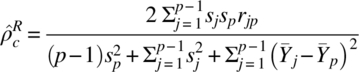
When Yαj are p measurements {Yα1, Yα2, …, Yαp} on the αth unit, generalizing CCC for p ≥ 2 is defined as
where μj and σj are the population mean and standard deviation of Yαj and ![]() is the population correlation coefficient of Yαj and
is the population correlation coefficient of Yαj and ![]() (Barnhart, Haber, and Song, 2002; Barnhart et al., 2007; King and Chinchilli, 2001; Lin, 1989). An estimate of ρc is
(Barnhart, Haber, and Song, 2002; Barnhart et al., 2007; King and Chinchilli, 2001; Lin, 1989). An estimate of ρc is

where ![]() and sj are the sample mean and standard deviation of sample Yαj and
and sj are the sample mean and standard deviation of sample Yαj and ![]() is the sample correlation coefficient of Yαj and
is the sample correlation coefficient of Yαj and ![]() .
.
Alternatively, Carrasco and Jover (2003) estimated CCC using variance components of a mixed effects model. Expressions for CCC adjusted by confounding covariates were provided by King and Chinchilli (2001).
When one of the methods, say p, is a gold standard method, the CCC, measuring the association of the other p − 1 variables with the gold standard method is defined as

and can be estimated by
interpreting the symbols as in the preceding text (Barnhart et al., 2007).
A numerical example will be provided using the three test scores given in Table 2.6.1. The SAS program and output for CCC for p ≥ 2 is provided as follows:
data a; input stdnum test1 test2 test3 @@; cards;

1 70 63 57 2 60 67 50 3 70 87 35 4 70 87 35 5 67 60 636 73 80 53 7 80 83 70 8 83 93 63 9 50 80 83 10 83 40 53

;

proc corr outp=out;var test1 test2 test3; run;

data mean;set out;if _type_='MEAN';
mean1=test1; mean2=test2;mean3=test3;
a=1;keep a mean1 mean2 mean3; proc sort;by a;

data stdev;set out;if _type_='STD';
stdev1=test1; stdev2=test2;stdev3=test3;
a=1;keep a stdev1 stdev2 stdev3; proc sort;by a;

data corr1;set out; if _type_='CORR' and _name_='test1' then do;
rho12= test2; rho13= test3; end; if rho12=. then delete;
a=1; keep a rho12 rho13 ;proc sort;by a;

data corr2;set out; if _type_='CORR' and _name_='test2' then do;
rho23= test3; end;  if rho23=. then delete;
a=1; keep a rho23;proc sort;by a;

data stats;merge mean stdev corr1 corr2;by a;

/***input data***/
p=3; * number of variables;
/***end of input data***/

num=2*(stdev1*stdev2*rho12+stdev1*stdev3*rho13+stdev2*stdev3*rho23);
den=(p-1)*(stdev1**2+stdev2**2+stdev3**2)+(mean1-mean2)**2+(mean1-mean3)**2+(mean2-mean3)**2;

CONCORR =num/den;
keep concorr; proc print; run;

             CONCORR
             −0.067845
The concordance correlation ranges from –1 to +1 and is usually positive. According to McBride (2005), the strength of agreement is considered poor (ρc < 0.9), moderate (0.90 ≤ ρc < 0.95), substantial (0.95 ≤ ρc < 0.99), and almost perfect (ρc ≥ 0.99).
In our example, the concordance correlation is –0.068, which is considered to be a poor association between the three test scores.
2.8 Multiresponse Concordance Correlation Coefficient
We will now generalize the concept of CCC to a multiple response situation. Let Yαi be a p-dimensional response vector of the ith method, devices, laboratories, observers, etc., on the αth unit, for α = 1, 2, …, n; i = 1, 2, …, k. Let

for i, j = 1, 2, …, k. Let


The multiresponse concondance correlation for the k methods is defined as

Equation (2.8.1) was obtained by replacing the variances in Equation (2.7.3) by the generalized variance. For an alternate definition, see King, Chinchilli, and Carrasco (2007).
We estimate μi, μj, ∑ ii, ∑ jj, ∑ ij, ∑ ji by
Replacing V1ij, V0ij by their estimates, we get the estimator of ρMc.
For illustration, we will now provide a numerical example.
Table 2.8.1 Systolic and diastolic BP for three treatments
| Subject | Treatment A | Treatment B | Treatment C | |||
| Systolic BP | Diastolic BP | Systolic BP | Diastolic BP | Systolic BP | Diastolic BP | |
| 1 | 140 | 80 | 160 | 85 | 130 | 70 |
| 2 | 150 | 75 | 155 | 82 | 135 | 75 |
| 3 | 145 | 70 | 165 | 80 | 140 | 75 |
| 4 | 155 | 77 | 158 | 82 | 145 | 85 |
| 5 | 152 | 76 | 150 | 83 | 140 | 70 |
The necessary programming lines and output are given as follows:
data a; input sysb1 diasb1 sysb2 diasb2 sysb3 diasb3 @@;cards;

140 80 160 85 130 70 150 75 155 82 135 75 145 70 165 80 140 75155 77 158 82 145 85 152 76 150 83 140 70

;

data cov;set a;
proc corr cov outp=stats noprint;
var sysb1 diasb1 sysb2 diasb2 sysb3 diasb3;
run;

data stats;set stats;
if _type_ ='COV' or _type_='MEAN';

proc iml; use stats;
read all into y var {sysb1 diasb1 sysb2 diasb2 sysb3 diasb3};

ms1=Y[7,1];*mean sysb1; ms2=Y[7,3];*mean sysb2; ms3=Y[7,5];*mean sysb3;
md1=Y[7,2];*mean diasb1; md2=Y[7,4];*mean diasb2; md3=Y[7,6];*mean diasb3;

a=y[1,1]; b=y[1,2]; c=y[2,2];
d=y[1,3]; e=y[1,4]; f=y[2,4];
g=y[1,5]; h=y[1,6]; i=y[2,6];
j=y[3,3]; k=y[3,4]; l=y[4,4];

m=y[5,5]; n=y[5,6]; o=y[6,6];
p=y[3,5]; q=y[3,6]; r=y[4,6];
s=y[2,3]; t=y[2,5]; u=y[4,5];

sigma11=(a||b)//(b||c); sigma22=(j||k)//(k||l); sigma33=(m||n)//(n||o);sigma12=(d||e)//(s||f); sigma13=(g||h)//(t||i); sigma23=(p||q)//(u||r);

mean1=(ms1||md1); mean2=(ms2||md2);
mean3=(ms3||md3);

v112=sigma11+sigma22-sigma12-sigma12`;v012=sigma11+sigma22+(mean1-mean2)`*(mean1-mean2);

v113=sigma11+sigma33-sigma13-sigma13`;v013=sigma11+sigma33+(mean1-mean3)`*(mean1-mean3);

v123=sigma22+sigma33-sigma23-sigma23`;v023=sigma22+sigma33+(mean2-mean3)`*(mean2-mean3);

rhoMc=1-((det(v112)+det(v113)+det(v123))/ (det(v012)+det(v013)+det(v023)));

print rhoMc ;quit;run;

   RHOMC
   0.8606674
According to McBride (2005), there is poor agreement between the treatments for the systolic and diastolic BP. This implies that the three treatment effects are not associated. This measure does not indicate which treatment is better in the treatment of BP.
2.9 Repeated Measurements with Binary Response
Let p repeated observations with binary (0 or 1) responses be taken on N experimental units. Let πi be the probability of response 1 at the ith observation, and we are interested in testing the null hypothesis
against the alternative hypothesis that not all πi’s are equal. An easy and a simple analysis is to form p − 1 contingency tables on the marginal distribution of 1st and ith responses (i = 2, 3, …, p − 1) and to test π1 = πi using McNemar’s test with a conservative α/(p − 1) level of significance.
Alternatively, let ![]() be the frequency of responses of the (i1, i2, …, ip) profile of the 2p possible outcomes and
be the frequency of responses of the (i1, i2, …, ip) profile of the 2p possible outcomes and ![]() be the probability of observing that profile. Stack the probabilities
be the probability of observing that profile. Stack the probabilities ![]() in a 2p column vector π*. Note
in a 2p column vector π*. Note
and ![]() is the column vector of
is the column vector of ![]() .
.
The estimated dispersion matrix of ![]() is
is
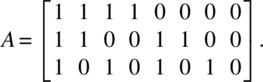
From a p × 2p matrix A, with the ith row consisting of 1’s if the ith period response is 1 in the jth profile (i = 1, 2, …, p; j = 1, 2, …, 2p). Let π be the column vector of π1, π2, …, πp. We then have
As defined earlier, let P1 be a (p − 1) × p matrix such that

is an orthogonal matrix. The null hypothesis (2.9.1) is equivalent to the null hypothesis
and it can be tested by using the test statistic
which is asymptotically distributed as a χ2 variable with (p − 1) degrees of freedom. We will now provide an example.
Table 2.9.1 Performance of students in three tests
| Tests | |||
| 1 | 2 | 3 | Frequency |
| P | P | P | 15 |
| P | P | F | 7 |
| P | F | P | 6 |
| P | F | F | 2 |
| F | P | P | 5 |
| F | P | F | 3 |
| F | F | P | 1 |
| F | F | F | 1 |
| Total | 40 | ||
Here, ![]() .
.
The matrix A is
The following SAS program provides the necessary output to test π1, π2, π3:
data a; input test1 test2 test3 count @@; cards;
1 1 1 15 1 1 0 7 1 0 1 6 1 0 0 2 0 1 1 5 0 1 0 3 0 0 1 1 0 0 0 1

;

proc catmod order=data;
weight count;
response marginals;
model test1*test2*test3=_response_/oneway;
repeated test 3/_response_=test;

contrast 'test1 vs test2' all_parms 1 -1 0 ;
contrast 'test1 vs test3' all_parms 1 0 -1;
contrast 'test2 vs test3' all_parms 0 1 -1; run;

                             ***

Analysis of Variance
Source   DF Chi-Square Pr > ChiSq
                              (b1)
Intercept  1   318.36  <.0001
test     2   0.77   0.6810
Residual    0    .     .

                              ***

Analysis of Contrasts
Contrast    DF Chi-Square Pr > ChiSq
                              (b2)
test1 vs test2   1  101.38  <.0001
test1 vs test3   1    86.47  <.0001
test2 vs test3   1     0.00    1.0000
In the output column (b1), the p-value for tests is 0.6810. This p-value is used to test the null hypothesis that the probability of passing the course in the three tests is the same. Since our p-value of 0.681 is greater than the level of significance, α = 0.05, we retain the null hypothesis that the equality of probabilities of passing the three tests is not rejected. The column (b2) gives the p-value for testing the contrasts effects. In our example, the first two contrasts are significant, indicating the rejection of the contrasts effects to be 0. This appears to be an example of overall nonsignificance of the effects and still rejecting some of the contrasts. However, tests 2 and 3 are not significantly different, indicating the validity of the overall nonsignificance of the three tests.
The simple analysis indicated at the beginning of this section is based on two marginal 2 × 2 contingency tables:
| Test 1 | Test 2 | Test 3 | ||
| P | F | P | F | |
| P | 22 | 8 | 21 | 9 |
| F | 8 | 2 | 6 | 4 |
The McNemar χ2 statistic for the two tables are 0 and 0.6, respectively, and are not significant each at the α level 0.05/2 = 0.025.
References
- Anderson, T. W. An Introduction to Multivariate Statistical Analysis. 2nd ed. New York: Wiley; 2003.
- Barnhart H, Haber M, Song J. Overall concordance correlation coefficient for evaluating agreement among multiple observers. Biometrics 2002;58:1020–1027.
- Barnhart H, Lokhnygina Y, Kosinski A, Haber, M. Comparison of concordance correlation coefficient and coefficient of individual agreement in assessing agreement. J Biopharm Stat 2007;19:721–738.
- Boik RJ. A priori tests in repeated measures designs. Effects of nonsphericity. Psychometrika 1981;46:241–255.
- Box GEP. A general distribution theory for a class of likelihood criteria. Biometrika 1949;36:317–346.
- Box GEP. Some theorems on quadratic forms applied in the study of analysis of variance problems, II. Effects of inequality of variances and correlation between errors in the two-way classification. Ann Math Statist 1954;25:484–498.
- Carrasco J, Jover L. Estimating the generalized concordance correlation coefficient through variance components. Biometrics 2003;59:849–858.
- Collier RO, Baker FB, Mandeville GK, Hays TF. Estimates of test size for several procedures based on conventional variance ratios in the repeated measure design. Psychometrika 1967;32:339–353.
- Consul PC. On the exact distribution of the criterion W for testing sphericity in a p-variate normal distribution. Ann Math Statist 1967;38:1170–1174.
- Geisser S, Greenhouse SW. An extension of Box’s results on the use of the F distribution in multivariate analysis. Ann Math Statist 1958;29:885–891.
- Greenhouse SW, Geisser S. On methods in the analysis of profile data. Psychometrika 1959;32:95–112.
- Huynh H. Some approximate tests for repeated measures designs. Psychometrika 1978;43:161–175.
- Huynh H, Feldt L. Estimation of the Box correction for degrees of freedom from sample data in randomized block and split-plot designs. J Edu Statist 1976;1:69–82.
- King T, Chinchilli V. A generalized concordance correlation coefficient for continuous and categorical data. Stats Med 2001;20:2131–2147.
- King T, Chinchilli V, Carrasco J. A repeated measures concordance correlation coefficient. Stats Med 2007;26:3095–3113.
- Lin LI-K. A concordance correlation coefficient to evaluate reproducibility. Biometrics 1989;45:255–268.
- Mauchley JW. Significance test for sphericity of a normal n-variate distribution. Ann Math Statist 1940;29:204–209.
- McBride GB. A proposal for strength-of-agreement criteria for Lin’s concordance correlation coefficient. NIWA Client Report: HAM2005-062; 2005.
- Mendoza JL, Toothaker LE, Nicewander WA. A Monte-Carlo comparison of the univariate and multivariate methods for the two-way repeated measures design. Multivariate Behav Res 1974;9:165–178.
- Rao CR. Linear Statistical Inference and its Applications. New York: Wiley; 1973.
- Rogan JC, Keselman HJ, Mendoza JL. Analysis of repeated measurements. Br J Math Stat Psychol 1979;32:269–286.
- Stoloff PH. Correcting for heterogeneity of covariance for repeated measures designs and the analysis of variance. Educ Psychol Meas 1970;30:909–924.
- Wilson K. The sampling distributions of conventional, conservative and corrected F ratio in repeated measurements designs with heterogeneity of covariance. J Statist Comp Simul 1975;3:201–215.