
Chapter 3
k-Sample Repeated Measurements Design
3.1 INTRODUCTION
This chapter generalizes the ideas developed in Chapter 2. Let there be k populations and let k-independent random samples be taken from these k populations. Let Yiα be the p-dimensional response vector on the αth unit from the ith population, α = 1, 2, …, Ni; i = 1, 2, …, k.
Let Yiα ~ IMNp(μi, ∑ i). Let ![]() . It is not necessary to have the observations taken from k populations. One may take N homogeneous units, randomly subdivide them into k sets of sizes N1, N2, …, Nk, assign the k treatments such that the ith treatment is assigned to each of the Ni experimental units of the ith set, and take p responses at the same time or at different time intervals. In either case, three kinds of null hypotheses are tested:
. It is not necessary to have the observations taken from k populations. One may take N homogeneous units, randomly subdivide them into k sets of sizes N1, N2, …, Nk, assign the k treatments such that the ith treatment is assigned to each of the Ni experimental units of the ith set, and take p responses at the same time or at different time intervals. In either case, three kinds of null hypotheses are tested:
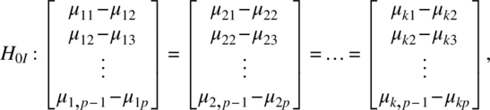
- Parallelism or interaction of the populations and responses
- Equality of population or group effects
- Equality of response or period effects
Let μ′i = (μi1, μi2, …, μip). The three kinds of null hypotheses can be represented as follows:


To test these three null hypotheses, we initially assume that ∑ 1 = ∑ 2 = … = ∑ k (=∑, say), and this assumption will be relaxed in Section 3.6. Further, if ∑ satisfies the sphericity condition, the conclusions can be drawn from the univariate ANOVA for a mixed model. Otherwise, multivariate methods can be used to analyze the data.
Test for the equality of dispersion matrices of the k populations will be discussed in Section 3.2. The univariate analysis of this problem will be given in Section 3.3, while the multivariate methods will be presented in Section 3.4. The methods discussed in Sections 3.2–3.4 will be illustrated in Section 3.5. The results with unequal dispersion matrices will be discussed in Section 3.6. Finally, in Section 3.7, we will discuss the analysis with ordered categorical responses.
3.2 Test for the Equality of Dispersion Matrices and Sphericity Condition Of k-Dispersion Matrices
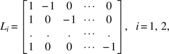
As indicated in Section 3.1, let Yiα ~ IMNp(μi, ∑i). Let P1 be a p–1 × p matrix such that
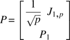
is an orthogonal matrix. Then,
where
The null hypothesis
is equivalent to
Let ![]()
![]() and
and ![]() . The likelihood function for testing the null hypothesis (3.2.5) is
. The likelihood function for testing the null hypothesis (3.2.5) is
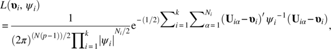
with likelihood ratio criterion

where the numerator is the maximum of the likelihood function over ω : {υi, ψ0|–∞ < υij < ∞, i = 1, 2, …, k, j = 1, 2, …, p – 1; d > 0} and the denominator is the maximum of the likelihood function over Ω: {υi, ψi|–∞ < υij < ∞, i = 1, 2, …, k, j = 1, 2, …, p – 1; ψi is positive definite}.
After some algebra, we obtain
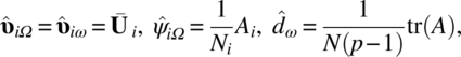
and Equation (3.2.7) simplifies to

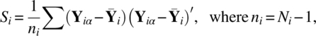
Following Bartlett (1937), we modify the test statistic λ to
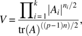
where ni = Ni–1 and ![]() .
.
Letting w(A;f, ∑) to be the Wishart density function of A with f degrees of freedom and population dispersion matrix ∑,

and by using the properties of Wishart and χ2 distributions, we can show that
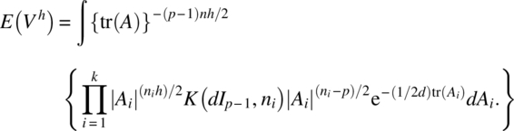


Using an asymptotic distribution of the likelihood ratio criterion of Box (1949), we can verify that

where

Thus, asymptotically, the critical region for testing the null hypothesis (3.2.5) is
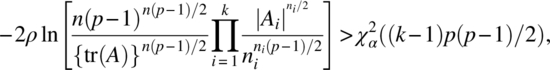
where ![]() is the upper α percentile point of the χ2 distribution with (k–1)p(p–1)/2 degrees of freedom.
is the upper α percentile point of the χ2 distribution with (k–1)p(p–1)/2 degrees of freedom.
3.3 Univariate ANOVA for k-Sample RMD
Let Yiαβ be the βth response on the αth unit of the ith sample (β = 1, 2,…, p; α = 1, 2, …, Ni; i = 1, 2, …, k). Clearly, Y′iα = (Yiα1, Yiα2, …, Yiαp).
We assume the linear model
where μ is the general mean; γi is the ith population effect if the sampling is done from k populations, or it is the effect of the ith treatment used on the Ni units; siα is the effect of the αth unit in the ith group; τβ is the βth response effect; δiβ is the interaction effect of the ith group (or treatment) with the βth response; and eiαβ are random errors. The model (3.3.1) is a mixed effects model in which siα and eiαβ are random effects. Putting e′iα = (eiα1, eiα2, …, eiαp), it is further assumed that
where ∑ satisfies the sphericity condition.
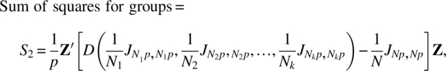
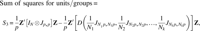
Letting ![]() the sum of squares arising from model (3.3.1) are the following:
the sum of squares arising from model (3.3.1) are the following:


Using Lemmas 2.3.1 and 2.3.2 and calling f as the sum of all elements of ∑, that is, f = J1,p ∑ Jp,1, ![]() ,
, ![]() , S3/f ~ χ2(N - k),
, S3/f ~ χ2(N - k), ![]() , and S5/d ~ χ2((p - 1)(N - k)). Further, the pairs of quadratic forms (S1, S5), (S2, S3), and (S4, S5) are independently distributed.
, and S5/d ~ χ2((p - 1)(N - k)). Further, the pairs of quadratic forms (S1, S5), (S2, S3), and (S4, S5) are independently distributed.
The noncentrality parameters δ1, δ2, and δ3 can be evaluated as in Section 2.3 to get
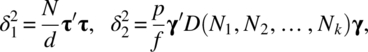
where τ ′ = (τ1, τ2, …, τp), γ ′ = (γ1, γ2, …, γk), and δ ′ = (δ11, δ12, …, δ1p, …, δk1, δk2, …, δkp).
Thus,
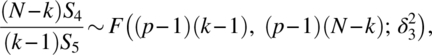
where ![]() is a noncentral F distribution, which reduces to the central F distribution under the null hypothesis (3.1.1). Thus, the critical region for testing the interactions between the groups and the responses given by the null hypothesis (3.1.1) is
is a noncentral F distribution, which reduces to the central F distribution under the null hypothesis (3.1.1). Thus, the critical region for testing the interactions between the groups and the responses given by the null hypothesis (3.1.1) is

Similarly, we note that the critical region for testing the equality of group effects given by the null hypothesis (3.1.2) is

and the critical region for testing the equality of response effects given by the null hypothesis (3.1.3) is

The analysis resulting from the earlier tests can be summarized in the k-sample RMD ANOVA (Table 3.3.1).
Table 3.3.1 k-Sample RMD ANOVA
| Source | d.f. | S.S. | M.S. | F |
| Responses | p–1 | S 1 | S 1/(p–1) | (N–k)S1/S5 |
| Groups | k–1 | S 2 | S 2/(k–1) | (N–k)S2/(k–1)S3 |
| Units/groups | N–k | S 3 | S 3/(N–k) | |
| Groups × responses | (k–1)(p–1) | S 4 | S 4/(k–1)(p–1) | (N–k)S4/(k–1)S5 |
| Error | (p–1)(N–k) | S 5 | S 5/(p–1)(N–k) | |
| Total | NP–1 | S 6 |
One can perform standard multiple comparison tests like Scheffe’s to test individual contrasts of responses or groups. When the sphericity condition is not satisfied for the common dispersion matrix, one can conservatively test the F statistics for responses with numerator and denominator degrees of freedom 1 and (p–1)(N–k).
3.4 Multivariate Methods for k-Sample RMD
Letting Yiα to be the p-component response vector on the αth observation (or unit) taken from the ith population (or treated with ith treatment), it is assumed that Yiα ∼ IMNp(μi, ∑) for α = 1, 2, …, Ni; i = 1, 2, …, k. Let L be a (p–1) × p matrix as defined in (2.4.1) and let
Then, clearly
where
and
The null hypothesis (3.1.1) is equivalent to
This is the standard multivariate ANOVA problem discussed in Rao (1973), Morrison (1976), and Anderson (2003) and can be solved using test statistics involving determinants or maximum eigenvalues of functions of matrices representing the hypotheses and error. Let

and
Put
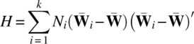
and

The matrices H and E are the hypothesis and error matrices for testing the null hypothesis (3.4.5).
Let s = min(k – 1, p – 1) and let cs be the greatest eigenvalue of HE-1. The upper percentage points of the greatest root distribution of the matrix H(H + E)- 1 have been computed by Heck (1960), Pillai and Bantegu (1959), and Pillai (1964, 1965, 1967). The maximum eigenvalue cs of HE-1 is related to the maximum eigenvalue θs of H(H + E)- 1 by the relation
Using ![]() ,
, ![]() , the upper α percentile point cα(s, m, n) of the distribution θs can be obtained from Heck’s charts or Pillai’s tables, and the critical region for testing the null hypothesis (3.4.5) is
, the upper α percentile point cα(s, m, n) of the distribution θs can be obtained from Heck’s charts or Pillai’s tables, and the critical region for testing the null hypothesis (3.4.5) is
Alternatively, one notes that

and can construct critical regions accordingly for testing the null hypothesis (3.4.5).Letting
it follows that the one-dimensional random variable Uiα has
and the null hypothesis (3.1.2) is based on the F statistic with (k – 1) and (N – k) degrees of freedom given by

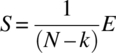
where

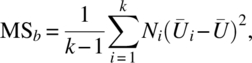
and

This can be summarized in Table 3.4.1.
Table 3.4.1 ANOVA for testing groups in a k-sample RMD
| Source | d.f. | S.S. | M.S. | F |
| Between groups | k – 1 |  |
MSb | MSb/MSe |
| Within groups | N – k |  |
MSe | |
| Total | N – 1 |  |
The critical region for testing the null hypothesis (3.1.2) is thus
where F is the F value from the ANOVA Table 3.4.1. This is the same as the test discussed for univariate ANOVA in Section 3.3.
When the null hypothesis (3.1.1) or equivalently (3.4.5) is tenable, to test the responses, let υ be the common υ1 = υ2 = … = υk. The null hypothesis (3.1.3) is then equivalent to
Now Wiα ~ IMNp–1(υ, ψ) and testing (3.4.19) can be done as described in Section 2.4. Letting E to be defined as in Equation (3.4.9), one notes that E ~ Wp–1(N–k, ψ).
Put
and
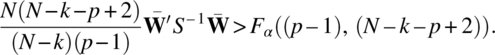
Under the null hypothesis (3.4.19)
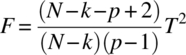
is distributed as an F distribution, with degrees of freedom (p – 1) and (N – k – p + 2). Thus, the critical region for testing the null hypothesis (3.1.3) is
3.5 Numerical Example
In this section, the methods discussed in Sections 3.2–3.4 will be illustrated through an example with artificial data for the situation considered in Example 1.3.2.
Table 3.5.1 Artificial data of ABS scores
| Groups | Periods | ||
| 1 | 2 | 3 | |
| 1 | 109 | 115 | 125 |
| 110 | 112 | 135 | |
| 105 | 102 | 100 | |
| 2 | 97 | 120 | 121 |
| 126 | 142 | 148 | |
| 151 | 197 | 189 | |
| 3 | 122 | 162 | 138 |
| 157 | 152 | 217 | |
| 212 | 235 | 213 | |
| 137 | 183 | 273 | |
| 4 | 225 | 204 | 197 |
| 175 | 181 | 203 | |
We assume that the dispersion matrices for the four groups are equal as we cannot test the equality of dispersion matrices for this example because the sample sizes in each group is not 1 more than the number of variables.
The following SAS program provides the necessary output:
data a;input patnum group period1 period2 period3 @@;cards;
1 1 109 115 125 2 1 110 112 135 31 105 102 100
4 2 97 120 121 5 2 126 142 148 6 2 151 197 189
7 3 122 162 138 8 3 157 152 217 9 3 212 235 213
10 3 137 183 273 11 4 225 204 197 12 4 175 181 203
;

proc glm;class group;
model period1 period2 period3=group/nouni;
*the nouni will not provide the univariate Anova for each dependent variable;
repeated period 3 profile /printe uepsdef= HF;run;
*The period indicates the label for the repeated measurements variable, 3 is the number of repeated measurement, profile is the type of transformation specified and printe provides a test for sphericity (see the SAS manual for further details);

data b;set a;
diff1=period1-period2;diff2=period2-period3;
*This is needed to study the linear and quadratic period effects across groups;
proc glm;class group;
model diff1 diff2=group/nouni;
repeated diff 2profile;run;
***
Sphericity Tests
Mauchly's
| Variables | DF | Criterion | Chi-Square | Pr > ChiSq |
| Transformed Variates | 2 | 0.5882072 | 3.7147324 | 0.1561 |
| Orthogonal Components | 2 | 0.457953 | 5.4669214 | 0.0650 (a1) |
The GLM Procedure
Repeated Measures Analysis of Variance
MANOVA Test Criteria and Exact F Statistics for the Hypothesis of no period Effect
H = Type III SSCP Matrix for period
E = Error SSCP Matrix
S=1 M=0 N=2.5
| Statistic | Value | F Value | Num DF | Den DF | Pr > F |
| Wilks' Lambda | 0.54657575 | 2.90 | 2 | 7 | 0.1207 (a2) |
| Pillai's Trace | 0.45342425 | 2.90 | 2 | 7 | 0.1207 |
| Hotelling-Lawley Trace | 0.82957256 | 2.90 | 2 | 7 | 0.1207 |
| Roy's Greatest Root | 0.82957256 | 2.90 | 2 | 7 | 0.1207 |
MANOVA Test Criteria and F Approximations for the Hypothesis of no period*group Effect
H = Type III SSCP Matrix for period*group
E = Error SSCP Matrix
S=2 M=0 N=2.5
| Statistic | Value | F Value | Num DF | Den DF | Pr > F |
| Wilks' Lambda | 0.43419217 | 1.21 | 6 | 14 | 0.3584 (a3) |
| Pillai's Trace | 0.62009838 | 1.20 | 6 | 16 | 0.3564 |
| Hotelling-Lawley Trace | 1.17808962 | 1.32 | 6 | 7.7895 | 0.3502 |
| Roy's Greatest Root | 1.06014535 | 2.83 | 3 | 8 | 0.1066 |
NOTE: F Statistic for Roy's Greatest Root is an upper bound.
NOTE: F Statistic for Wilks' Lambda is exact.
The GLM Procedure
Repeated Measures Analysis of Variance
Tests of Hypotheses for Between Subjects Effects
| Source | DF | Type III SS | Mean Square | F Value | Pr > F |
| group | 3 | 37607.02778 | 12535.67593 | 5.50 | 0.0240 (a4) |
| Error | 8 | 18234.86111 | 2279.35764 |
The GLM Procedure
Repeated Measures Analysis of Variance
Univariate Tests of Hypotheses for Within Subject Effects4
Adj Pr > F
| Source | DF | Type III SS | Mean Square | F Value | Pr > F | G – G | H – F |
| period | 2 | 3070.676471 | 1535.338235 | 2.74 | 0.0949(a5) | 0.1230(a6) | 0.0949 (a7) |
| period*group | 6 | 2958.555556 | 493.092593 | 0.88 | 0.5317(a8) | 0.5064 (a9) | 0.5317(a10) |
| Error(period) | 16 | 8972.388889 | 560.774306 |
Greenhouse-Geisser Epsilon 0.6485 (a11)
Huynh-Feldt Epsilon 1.0118(a12)
***
MANOVA Test Criteria and Exact F Statistics for the Hypothesis of no diff*group Effect
H = Type III SSCP Matrix for diff*group
E = Error SSCP Matrix
S=1 M=0.5 N=3
| Statistic | Value | F Value | Num DF | Den DF | Pr > F |
| Wilks' Lambda | 0.82126201 | 0.58 | 3 | 8 | 0.6442 (a13) |
| Pillai's Trace | 0.17873799 | 0.58 | 3 | 8 | 0.6442 |
| Hotelling-Lawley Trace | 0.21763820 | 0.58 | 3 | 8 | 0.6442 |
| Roy's Greatest Root | 0.21763820 | 0.58 | 3 | 8 | 0.6442 |
The GLM Procedure
Repeated Measures Analysis of Variance
Tests of Hypotheses for Between Subjects Effects
| Source | DF | Type III SS | Mean Square | F Value | Pr > F |
| group | 3 | 2442.750000 | 814.250000 | 0.99 | 0.4464 (a14) |
| Error | 8 | 6602.375000 | 825.296875 |
***
In the output at (a1), we have the p-value to test the sphericity condition of the dispersion matrices (Mauchly, 1940). If this p-value is more than 0.05, the sphericity assumption is not rejected. In our example, it is 0.065 and the sphericity condition is valid and hence the univariate approach can be used to test the hypothesis. At (a5) and (a8), we have the p-values for testing the period effect and the period*group interaction effect. In our example, these are not significant. Had the sphericity condition been rejected, p-values given at (a6) and (a9) adjusting by the method of Greenhouse and Geisser or the p-values given at (a7) and (a10) adjusting by the method of Huynh and Feldt could have been used. In our problem, these p-values are also not significant. The Greenhouse and Geisser (1959) adjustment ![]() is given at (a11) and is 0.6485. The Huynh and Feldt (1976) adjustment
is given at (a11) and is 0.6485. The Huynh and Feldt (1976) adjustment ![]() is given at (a12) and is 1.0118.
is given at (a12) and is 1.0118.
Note that instead of the Huynh–Feldt epsilon, the Lecoutre correction of the Huynh–Feldt epsilon is displayed as a default for SAS releases from 9.22 onwards. The Huynh–Feldt epsilon’s numerator is precisely unbiased only when there are no between-subject effects. Lecoutre (1991) made a correction to the numerator of the Huynh–Feldt epsilon. However, one can still request Huynh–Feldt epsilon by using the option UEPSDEF = HF in the REPEATED statement.
In our example, the Huynh–Feldt–Lecoutre epsilon is 0.7215. The p-values for period and period*group adjusting by the method of Huynh–Feldt–Lecoutre are 0.1167 and 0.5126.
By using the multivariate methods, the p-value at (a2) will be used to test the no period effect hypothesis and the p-value at (a3) to test the interaction effect of period and groups. The p-value at (a4) is used to test the group effect in univariate or multivariate analyses. In our example, this p-value is significant, and hence, the ABS scores differ in the four groups.
If the periods are of equal time intervals, the linear and quadratic effects of periods can be tested by using the p-values at (a13) and (a14). The linear effect equality across groups is tested by the p-value given at (a14), and it is not significant in our example. The quadratic effect equality across groups of the periods can be tested by the p-value given at (a13) and is not significant.
For further programming details, see the SAS manual.
3.6 Multivariate Methods with Unequal Dispersion Matrices
Continuing the notation used in this chapter so far, let Yiα be distributed IMNp(μi, ∑ i) for α = 1, 2, …, Ni; i = 1, 2, …, k. Put

where L1 is (k–1) × k and L2 is (p–1) × p matrices. Further, D(…) is a block diagonal matrix with entries in the diagonal position. Note that the rows of C1μ are independent contrasts of groups and period interaction, C2μ are independent contrasts of groups, and C3μ are independent contrasts of periods. Following Welch (1947, 1951) and James (1951, 1954), the three null hypotheses (3.1.1), (3.1.2), and (3.1.3) can be tested using the test statistics:
Let q = kp, m1 = (p–1)(k–1), m2 = k–1, m3 = p–1,
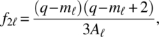
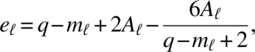
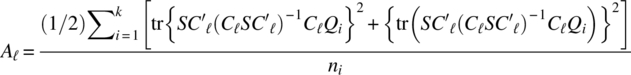
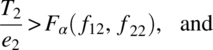
for ![]() , where Qi is a kp square block matrix whose (u, w) is Ip for u = w = i and 0 for u ≠ w; u, w = 1, 2, …, k. The critical regions for testing the hypotheses (3.1.1), (3.1.2), and (3.1.3) are, respectively,
, where Qi is a kp square block matrix whose (u, w) is Ip for u = w = i and 0 for u ≠ w; u, w = 1, 2, …, k. The critical regions for testing the hypotheses (3.1.1), (3.1.2), and (3.1.3) are, respectively,


For some simulation results, see Keselman, Carriere, and Lix (1993). Also, see Keselman, Algina, and Kowalchuk (2001) for a review on repeated measurements designs.
Let us continue with the ABS scores data given in Table 3.5.1. Though the dispersion matrices for the four groups are not significantly different, we will still use the test discussed in this section.
data a;input patnum group period1 period2 period3 @@;cards;
1 1 109 115 125 2 1 110 112 135 3 1 105 102 100 4 2 97 120 121
5 2 126 142 148 6 2 151 197 189 7 3 122 162 138 8 3 157 152 217
9 3 212 235 213 10 3 137 183 273 11 4 225 204 197 12 4 175 181 203
;
proc sort;by group;
proc corr cov outp=stats noprint; var period1 period2 period3;by group ;run;

data stats;set stats;
proc iml;use stats;
read all into y var{period1 period2 period3};

meany=
{108.00 109.67 120.0 124.67 153.00 152.67 157.00 183. 00 210.25 200.00 192.50 200.00};

l1={1 –1 0 0,1 0 - 1 0,1 0 0 -1};
l2={1 –1 0,1 0 –1};

j1={1 1 1}; j2={1 1 1 1};
c1= l1@l2; *l1 kronecker product l2;
c2=l1@j1;
c3=j2@l2;

/***input data***/

k=4;*number of groups;
p=3;*number of periods;

/*** end of input data ***/

q=k*p;
m1=(p-1)*(k-1);
m2=k-1;
m3=p-1;

f11= q - m1;
f12 = q - m2;
f13 = q - m3;

s1=y[1:3,1:3];
s2=y[10:12,1:3];
s3=y[19:21,1:3];
s4=y[28:30,1:3];
s=block(s1,s2,s3,s4);*S=D(s1,s2,s3,s4);

T1=(C1*meany`)`*(inv(c1*s*C1`))*(c1*meany`);T2=(C2*meany`)`*(inv(c2*s*C2`))*(c2*meany`);
T3=(C3*meany`)`*(inv(c3*s*C3`))*(c3*meany`);
zero={0 0 0 ,0 0 0 ,0 0 0};
q1=block(I(3),zero,zero,zero);*create a block matrix;
q2=block(zero,I(3),zero,zero);
q3=block(zero,zero,I(3),zero);
q4=block(zero,zero,zero,I(3));

/**A1**/

d11= (s*c1`)*(inv(c1*s*c1`))*(c1*q1);
a11=(trace(d11*d11)+(trace(d11))**2)/2;
d12= (s*c1`)*(inv(c1*s*c1`))*(c1*q2);
a12=(trace(d12*d12)+(trace(d12))**2)/2;
d13= (s*c1`)*(inv(c1*s*c1`))*(c1*q3);
a13=(trace(d13*d13)+(trace(d13))**2)/3;
d14= (s*c1`)*(inv(c1*s*c1`))*(c1*q4);
a14=(trace(d14*d14)+(trace(d14))**2)/1;a1=(a11+a12+a13+a14)/2;

/**A2**/
d21= (s*c2`)*(inv(c2*s*c2`))*(c2*q1);
a21=(trace(d21*d21)+(trace(d21))**2)/2;
d22= (s*c2`)*(inv(c2*s*c2`))*(c2*q2);
a22=(trace(d22*d22)+(trace(d22))**2)/2;
d23= (s*c2`)*(inv(c2*s*c2`))*(c2*q3);
a23=(trace(d13*d13)+(trace(d13))**2)/3;
d24= (s*c2`)*(inv(c2*s*c2`))*(c2*q4);
a24=(trace(d14*d14)+(trace(d14))**2)/1;
a2=(a21+a22+a23+a24)/2;

/**A3**/
d31= (s*c3`)*(inv(c3*s*c3`))*(c3*q1);
a31=(trace(d31*d31)+(trace(d31))**2)/2;d32= (s*c3`)*(inv(c3*s*c3`))*(c3*q2);
a32=(trace(d32*d32)+(trace(d32))**2)/2;
d33= (s*c3`)*(inv(c3*s*c3`))*(c3*q3);
a33=(trace(d33*d33)+(trace(d33))**2)/3;
d34= (s*c3`)*(inv(c3*s*c3`))*(c3*q4);
a34=(trace(d34*d34)+(trace(d34))**2)/1;
a3=(a31+a32+a33+a34)/2;

f21=((q-m1)*(q-m1+2))/3*a1;
f22=((q-m2)*(q-m2+2))/3*a2;
f23=((q-m3)*(q-m3+2))/3*a3;
e1=q-m1+2*a1-((6*a1)/(q-m1+2));
e2=q-m2+2*a2-((6*a2)/(q-m2+2));
e3=q-m3+2*a3-((6*a3)/(q-m3+2));

p1=1-probf(t1/e1,f11,f21);*p-value for the interaction;
p2=1-probf(t2/e3,f12,f22);*p-value for the groups;
p3=1-probf(t3/e3,f13,f23); *p-value for the responses;
print p1 p2 p3;quit;run;
| p1 | p2 | p3 |
| 0.7137978 | 0.030452 | 0.9919797 |
From the output, the p-values p1, p2, and p3 are used to test the significance of the interaction, groups, and responses. Our values indicate the interaction is not significant. Hence, we can test for the groups and responses and we observe the groups p-value is significant, whereas the responses p-value is not significant.
3.7 Analysis with Ordered Categorical Response
In some cases, the response Yiαβ taken at βth period on the αth unit of the ith group takes any of c-ordered categorical responses for β = 1, 2, …, p; α = 1, 2 …, Ni, i = 1, 2, …, k. To illustrate, let us consider the data given in Table 3.5.1 and let us convert it into an ordered categorical data with three categories defined by a: <110; b: [110, 150]; c: ≥150 to obtain Table 3.7.1.
Table 3.7.1 Data of Table 3.5.1 with ordered categorical response
| Periods | |||
| Groups | 1 | 2 | 3 |
| 1 | a | b | b |
| b | b | b | |
| a | a | a | |
| 2 | a | b | b |
| b | b | b | |
| c | c | c | |
| 3 | b | c | b |
| c | c | c | |
| c | c | c | |
| b | c | c | |
| 4 | c | c | c |
| c | c | c | |
Let ![]() be the responses in the p periods, where
be the responses in the p periods, where ![]() = 1, 2, …, c for β = 1, 2, …, p and let
= 1, 2, …, c for β = 1, 2, …, p and let ![]() be the probability of getting responses
be the probability of getting responses ![]() , for the ith group. For each i = 1, 2, …, k, we get cp joint probabilities. We define the marginal probabilities:
, for the ith group. For each i = 1, 2, …, k, we get cp joint probabilities. We define the marginal probabilities:

We estimate these probabilities from the data. From Table 3.7.1, we construct Table 3.7.2, giving the marginal probabilities in parentheses.
Table 3.7.2 Marginal estimated probabilities for the data of Table 3.7.1
| Period1 | Period 2 | Period 3 | |||||||
| Groups | a | b | c | a | b | c | a | b | c |
| 1 | 2 (2/3) | 1 (1/3) | 0 (0) | 1 (1/3) | 2 (2/3) | 0 (0) | 1 (1/3) | 2 (2/3) | 0 (0) |
| 2 | 1 (1/3) | 1 (1/3) | 1 (1/3) | 0 (0) | 2 (2/3) | 1 (1/3) | 0 (0) | 2 (2/3) | 1 (1/3) |
| 3 | 0 (0) | 2(2/4) | 2 (2/4) | 0 (0) | 0 (0) | 4 (1) | 0 (0) | 1 (1/4) | 3 (3/4) |
| 4 | 0 (0) | 0 (0) | 2 (1) | 0 (0) | 0 (0) | 2 (1) | 0 (0) | 0 (0) | 2 (1) |
We will now discuss the cumulative logit analysis of the marginal probabilities here, and for other models of analyses, the interested reader is referred to Kenward and Jones (1992).
We consider the (c – 1) logits


and may model
where ![]() is the general mean,
is the general mean, ![]() is the ith group effect,
is the ith group effect, ![]() is the βth period effect, and
is the βth period effect, and ![]() is the interaction effect of ith group and jth period effects.
is the interaction effect of ith group and jth period effects.
However, it is preferable to assume ![]() ,
, ![]() , and
, and ![]() , and this assumption is known as proportional odds model. Under the proportional odds model,
, and this assumption is known as proportional odds model. Under the proportional odds model,
For the data of Table 3.7.2, the following program produces the necessary output to draw inferences on the interaction, groups, and periods effects:
data a;input period group score freq @@;cards;
1 1 1 2 1 1 2 1 1 1 3 0 2 1 1 1 2 1 2 2 2 1 3 0 3 1 1 1 3 1 2 2 3 1 3 0 1 2 1 1 1 2 2 1 1 2 3 1

2 2 1 0 2 2 2 2 2 2 3 1 3 2 1 0 3 2 2 2 3 2 3 1 1 3 1 0 1 3 2 2 1 3 3 2 2 3 1 0 2 3 2 0 2 3 3 4

3 3 1 0 3 3 2 1 3 3 3 3 1 4 1 0 1 4 2 0 1 4 3 2 2 4 1 0 2 4 2 0 2 4 3 2 3 4 1 0 3 4 2 0 3 4 3 2

;

data b;set a;
proc logistic descending; freq freq;
model score=period group period*group; run;***
Model Convergence Status
Convergence criterion (GCONV=1E-8) satisfied.
Score Test for the Proportional Odds Assumption
| Chi-Square | DF | Pr > ChiSq |
| 1.3236 | 3 | 0.7235 (b1) |
***
Testing Global Null Hypothesis: BETA=0
| Test | Chi-Square | DF | Pr > ChiSq |
| Likelihood Ratio | 28.4374 | 3 | <.0001 (b2) |
| Score | 20.7295 | 3 | 0.0001 (b3) |
| Wald | 14.4425 | 3 | 0.0024 (b4) |
Analysis of Maximum Likelihood Estimates
| Parameter | DF | Estimate | Standard Error | WaldChi-Square | Pr > ChiSq |
| Intercept 3 | 1 | –7.1453 | 3.0235 | 5.5848 | 0.0181 (b5) |
| Intercept 2 | 1 | –3.4946 | 2.6724 | 1.7101 | 0.1910 (b6) |
| period | 1 | 0.6202 | 1.2543 | 0.2445 | 0.6210 (b7) |
| group | 1 | 2.3951 | 1.2456 | 3.6973 | 0.0545 (b8) |
| period*group | 1 | 0.0113 | 0.5766 | 0.0004 | 0.9843 (b9) |
Association of Predicted Probabilities and Observed Responses
| Percent Concordant | 87.1 | Somers'D | 0.794 |
| Percent Discordant | 7.7 | Gamma | 0.837 |
| Percent Tied | 5.1 | Tau-a | 0.490 |
| Pairs | 389 | c | 0.897(b10) |
From the p-value of 0.7235 given at (b1), we observe that the proportional odds model is valid in this setting. From the value 0.897 given at (b10) for c, we observe the model is a good fit. The overall significance of the parameters is tested by the p-values given at (b2), (b3), or (b4), and all of these p-values indicate strong significance for all of the parameters. The p-value for interaction given at (b9) is not significant. The p-value for the period effects given at (b7) is not significant. However, the p-value for the groups given at (b8) indicates a borderline nonsignificance. By using the DESCENDING option in PROC LOGISTIC, the ith intercept corresponds to the ith or higher category of the response versus the categories less than i, and the p-value corresponding to the intercept i can be used to test its significance. In our problem, the p-value corresponding to (b5) is significant, indicating that the intercept term corresponding to the third category versus the first and second categories is significant. Similarly, the p-value corresponding to (b6) is not significant, indicating that the intercept corresponding to the second and third categories versus the first category is not significant.
References
- Anderson TW. An Introduction to Multivariate Statistical Analysis. 2nd ed. New York: Wiley; 2003.
- Bartlett MS. Properties of sufficiency and statistical tests. Proc R Soc 1937;160A:268–282.
- Box GEP. A general distribution theory for a class of likelihood criteria. Biometrika 1949;36:317–346.
- Greenhouse SW, Geisser S. On methods in the analysis of profile data. Psychometrika 1959;32:95–112.
- Heck DL. Charts of some upper percentage points of the distribution of the largest characteristic root. Ann Math Statist 1960;31:625–642.
- Huynh H, Feldt L. Estimation of the Box correction for degrees of freedom from sample data in randomized block and split plot designs. J Edu Statist 1976;1:69–82.
- James GS. The comparison of several groups of observations when the ratios of the population variances are unknown. Biometrika 1951;38:324–329.
- James GS. Tests of linear hypotheses in univariate and multivariate analysis when the ratios of population variances are unknown. Biometrika 1954;41:19–43.
- Kenward MG, Jones B. Alternative approaches to the analysis of binary and categorical repeated measurements. J Biopharm Statist 1992;2:137–170.
- Keselman H, Carriere K, Lix LM. Testing repeated measures hypotheses when covariance matrices are heterogeneous. J Educ Behav Statist 1993;18:305–319.
- Keselman H, Algina J, Kowalchuk R. The analysis of repeated measurements designs: a review. Br J Math Statist Psychol 2001;54:1–20.
- Lecoutre B. A correction for the epsilon approximate test with repeated measures design with two or more independent groups. J Edu Statist 1991;16:371–372.
- Mauchley JW. Significance test for sphericity of a normal n-variate distribution. Ann Math Statist 1940;29:204–209.
- Morrison DF. Multivariate Statistical Methods. 2nd ed. New York: McGraw Hill; 1976.
- Pillai KCS. On the distribution of the largest of seven roots of a matrix in multivariate analysis. Biometrika 1964;51:270–275.
- Pillai KCS. On the distribution of the largest characteristic root of a matrix in multivariate analysis. Biometrika 1965;52:405–414.
- Pillai KCS. Upper percentage points of the largest root of a matrix in multivariate analysis. Biometrika 1967;54:189–194.
- Pillai KCS, Bantegu CG. On the distribution of the largest of six roots of a matrix in multivariate analysis. Biometrika 1959;46:237–270.
- Rao CR. Linear Statistical Inference and Its Applications. 2nd ed. New York: Wiley; 1973.
- Welch BL. On the comparison of several mean values: An alternative approach. Biometrika 1951;38:330–336.
- Welch BL. The generalization of student’s problem when several different population variances are involved. Biometrika 1947;34:28–35.