
Chapter 5
Cross-Over Designs without Residual Effects
5.1 INTRODUCTION
When several treatments are tested in an experiment, it is economical and efficient to use sequences of treatments on each experimental unit. In such cases, the treatment differences can be more accurately estimated by eliminating the differences in experimental units.
Consider an experiment in which v treatments are tested on b experimental units. Let the duration of the experiment be suitably divided into k periods for application of treatments. Each of the v treatments can be used on each experimental unit, or a subset of the v treatments can be used on each experimental unit depending on the relative sizes of v and k. With v = 4 = k = b, using treatments A, B, C, and D, the experimental layout may appear as in Table 5.1.1.
Table 5.1.1 Design for v = b = k = 4
| Period | Experimental unit | |||
| 1 | 2 | 3 | 4 | |
| 1 | A | B | C | D |
| 2 | B | A | D | C |
| 3 | C | D | A | B |
| 4 | D | C | B | A |
In the layout of Table 5.1.1, unit 1 receives treatments A, B, C, and D in that order in the four periods; unit 2 receives treatments B, A, D, and C in that order in the four periods; etc. With v = 7, k = 3, b = 7, an experimental layout is given in Table 5.1.2.
Table 5.1.2 Design for v = b = 7, k = 3
| Period | Experimental unit | ||||||
| 1 | 2 | 3 | 4 | 5 | 6 | 7 | |
| 1 | A | B | C | D | E | F | G |
| 2 | B | C | D | E | F | G | A |
| 3 | D | E | F | G | A | B | C |
In the layout of Table 5.1.2, unit 1 receives treatments A, B, and D in that order of the seven treatments A–G; unit 2 receives treatments B, C, and E in that order; etc.
Since a sequence of treatments are applied on each experimental unit and the treatments are changed during the course of the experimentation, in the literature, this class of designs are called cross-over designs, change-over designs, or switch-over designs. In this monograph, they will be referred to as cross-over designs.
In cross-over designs, it is possible that the treatments may produce direct effects in the period of its application and residual effects in the periods after its application is discontinued. The residual effect of a treatment in the ith period after its application will be called ith-order residual effect. Usually though not always, the ith-order residual effect will be smaller than the (i – 1)th-order residual effect, and thus, in many experimental situations, one ignores the second- and higher-order residual effects.
The linear model used to analyze these designs should either incorporate a term accounting for the residual effects, or the experimenter should conduct the experiment and collect the data in such a manner that there is a reasonable washout period between successive applications of the treatments and the times of collecting the data for each treatment. In the washout period, the unit will not receive any treatment so that the effect of the treatment used in the previous period washes out.
Designs using washout periods, which do not account for residual effects, will be referred to as CODWOR, while cross-over designs where no washout periods are provided between periods and residual effects are accounted in the model will be referred to as CODWR.
CODWOR designs will be discussed in this chapter, while CODWR designs will be discussed in Chapters 6–8.
5.2 Fixed Effects Analysis of CODWOR
As mentioned in the introduction, CODWOR designs will now be considered using v treatments in k periods on b experimental units. The layout can be conveniently represented in a k × b array using v symbols, where the units correspond to the columns, rows to the periods, and symbols to the treatments. These designs are known in statistical design literature as row–columns designs, designs eliminating heterogeneity in two directions, or two-way elimination of heterogeneity designs.
Designs eliminating heterogeneity are available in a more general setting where some cells are untreated by the experimental treatments, and/or some cells receive multiple treatments. However, such generalized two-way elimination heterogeneity designs may not be usually appropriate as repeated measurements designs, as there is no need to provide an extra rest period for an experimental unit because a washout period was already provided in the experimental protocol. Furthermore, if a unit washes out or dies in the course of the experiment, such designs do not fall into the framework of a generalized two-way elimination of heterogeneity designs. Thus, attention is given in this chapter to designs where every cell is filled and the interested readers on generalized two-way elimination of heterogeneity designs are referred to Agrawal (1966a–c), Freeman and Jeffers (1962), and Pothoff (1962). Two-way Anova designs with multiple observations per cell may not be appropriate as RMD designs. However, allowances are made for using a treatment more than once on a unit in different periods.
The designs considered in this chapter will be written as a k × b square array where each cell is filled with one of the v symbols {1, 2, …, v}. Here, the columns correspond to the experimental units, rows to the periods, and symbols to the treatments. Let d(i, j) be the symbol used in the ith row and jth column. Let the ith symbol be replicated ri times and let r′ = (r1, r2, …, rv). If Yij is the observation taken in the ith period on the jth unit, it is assumed that
where μ is the general mean, ρi is the ith row (or period) effect, γj is the jth column (or unit) effect, τd(i,j) is the treatment effect of the treatment d(i, j), and eij are random errors assumed to be IIN(0, σ2). Note that γj’s may be random effects if the experimental units are randomly selected from the population of experimental units and the results in this direction will be discussed in Section 5.9. In this section, we restrict ourselves to the situation where the units are not randomly selected and γj’s are fixed effects.
Let ρ′ = (ρ1, ρ2, …, ρk), γ′ = (γ1, γ2, …, γb), τ′ = (τ1, τ2, …, τv), and Y′ = (Y11, Y12, …, Y1b, Y21, …, Y2b, …, Yk1, …, Ykb). Let U be a kb × v matrix whose ![]() position is 1 if the
position is 1 if the ![]() treatment is applied in the (i, j) cell and 0 otherwise. Equation (5.2.1) can be rewritten as
treatment is applied in the (i, j) cell and 0 otherwise. Equation (5.2.1) can be rewritten as
Let ![]() , where
, where ![]() is the number of times the ith treatment occurs in the jth row and let Mv,b = (mij), where mij is the number of times the ith treatment occurs in the jth column. Matrices L and M are, respectively, known as treatment-row and treatment-column incidence matrices.
is the number of times the ith treatment occurs in the jth row and let Mv,b = (mij), where mij is the number of times the ith treatment occurs in the jth column. Matrices L and M are, respectively, known as treatment-row and treatment-column incidence matrices.
The normal equations for the model (5.2.2) can be easily obtained and are

where D(r) denotes a diagonal matrix with diagonal entries, r1, r2, …, rv, G is the grand total, P is the k × 1 vector of row totals Pi, C is the column vector of column totals Cj, T is the column vector of treatment totals ![]() of responses, and ‘
of responses, and ‘![]() ’ over a parameter denotes its least squares estimator. The notation Cα|β,γ,… will be used throughout this monograph to denote the coefficient matrix of
’ over a parameter denotes its least squares estimator. The notation Cα|β,γ,… will be used throughout this monograph to denote the coefficient matrix of ![]() in the reduced normal equations after eliminating the parameter vectors included in the subscript(s) after the bar and ignoring the parameter vectors not listed in the subscripts, but are present in the model. The parameter μ is obviously eliminated, but will not be used as a subscript of C. Similar interpretation will be given to the adjusted treatment totals Qα|β,γ,…. Clearly, LJk,1 = r, J1,vL = bJ1,k, MJb,1 = r, J1,vM = kJ1,b, J1,kP = J1,bC = J1,vT = G.
in the reduced normal equations after eliminating the parameter vectors included in the subscript(s) after the bar and ignoring the parameter vectors not listed in the subscripts, but are present in the model. The parameter μ is obviously eliminated, but will not be used as a subscript of C. Similar interpretation will be given to the adjusted treatment totals Qα|β,γ,…. Clearly, LJk,1 = r, J1,vL = bJ1,k, MJb,1 = r, J1,vM = kJ1,b, J1,kP = J1,bC = J1,vT = G.
The second Equation of (5.2.3) can be solved for ![]() to get
to get
Substituting for ![]() in the third Equation of (5.2.3) and simplifying, we obtain
in the third Equation of (5.2.3) and simplifying, we obtain

where
Since ![]() , from Equation (5.2.5), we have
, from Equation (5.2.5), we have

Substituting for ![]() and
and ![]() in the fourth Equation of (5.2.3) and simplifying, the reduced normal equations estimating
in the fourth Equation of (5.2.3) and simplifying, the reduced normal equations estimating ![]() are given by
are given by
where
and
The residual sum of squares for the model (5.2.2) is

with (b – 1)(k – 1) – Rank(Cτ|ρ,γ), degrees of freedom. When Rank(Cτ|ρ,γ) = v – 1, all elementary contrasts of treatment effects are estimable and the design is said to be connected. The connectedness property for CODWOR will be discussed in Section 5.3.
The null hypothesis of main interest to the experimenter is
The restricted model then becomes
where μ* = μ + a, and after some routine algebra, the residual sum of squares of the restricted model is given by

with (b – 1) (k – 1), degrees of freedom. Thus, the sum of squares for testing the null hypothesis (5.2.12) is given by
with Rank(Cτ|ρ,γ) degrees of freedom. From the linear estimation theory (see Rao 1973, p. 191), we use

as a critical region for testing H0τ, where υ1 = Rank(Cτ|ρ,γ), υ2 = (b – 1)(k – 1) – Rank(Cτ|ρ,γ) and Fα(υ1, υ2) is the upper α percentile point of the F distribution. These results can be summarized in the Anova Table 5.2.1.
Table 5.2.1 Anova table for CODWOR
| Source | d.f. | S.S. | M.S. | F |
| Rows (ig. treat) | k – 1 |  |
||
| Columns (ig. treat) | b – 1 |  |
||
| Treatments (el. rows, col) | υ 1 | MSt | MSt/MSe | |
| Error | υ 2 | By subtraction (=E, say) | MSe | |
| Total | bk – 1 |  |
MSt = ![]() ′Qτ|ρ,γ/υ1, MSe = E/υ2, υ1 = Rank(Cτ|ρ,γ), υ2 = (b – 1)(k – 1) – υ1.
′Qτ|ρ,γ/υ1, MSe = E/υ2, υ1 = Rank(Cτ|ρ,γ), υ2 = (b – 1)(k – 1) – υ1.
As noted earlier, not all contrasts of treatment effects are estimable for every design.
Since Cτ|ρ,γJv,1 = Ov,1, if ![]() is estimable, then
is estimable, then ![]() . It can be easily seen that
. It can be easily seen that ![]() is estimable iff
is estimable iff ![]() . If
. If ![]() is estimable, then its best linear unbiased estimate (b.l.u.e.) is
is estimable, then its best linear unbiased estimate (b.l.u.e.) is
with variance
Thus, the null hypothesis
when ![]() is estimable, can be tested by using the t-statistic
is estimable, can be tested by using the t-statistic

with υ2 degrees of freedom for all real values a. Scheffe’s method of multiple comparisons can be used for drawing inferences about several contrasts.
To test the null hypothesis of equality of column effects given by
we eliminate ![]() ,
, ![]() , and
, and ![]() , in that order in Equation (5.2.3) to get
, in that order in Equation (5.2.3) to get
where


Cτ|ρ and Qτ|ρ being, respectively, given by
The sum of squares for testing the null hypothesis (5.2.21) will then be given by
with Rank(Cγ|ρ,τ) = υ3 degrees of freedom. The critical region for testing H0γ is then given by

Putting


the reduced normal equations for estimating ![]() are
are
and the sum of squares for testing
is given by
with Rank(Cρ|γ,τ) = υ4 degrees of freedom. The critical region for testing H0ρ is then given by

5.3 Connectedness in CODWOR
The following definition holds in any multifactor experiment:
A CODWOR with treatments connected is also known as a doubly connected design. The following theorem characterizes this property in terms of the rank of Cτ|ρ,γ:
A chain condition characterizing the connectedness property in a general multifactor design was given by Srivastava and Anderson (1970) and can be specialized for doubly connected designs. However, this condition is not as easy as it is in block designs to apply.
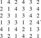
If a CODWOR is doubly connected, by putting γ = 0 identically in the model, it can be easily verified that all the contrasts of treatments effects are estimable if the design eliminates heterogeneity through rows only. Similarly, the contrasts of treatment effects are estimable if the design eliminates heterogeneity through columns only if ρ = 0. In looking at the converse of this problem, Federer and Zelen (1964) conjectured that an equireplicated CODWOR, in which the row design is connected and the column design is connected, is doubly connected. This conjecture was shown to be false by Shah and Khatri (1973) who gave the following counter example:

While the usual method of showing that the design (5.3.4) is not doubly connected rests on calculating Cτ|ρ,γ and showing that its rank is <7, the method adopted by Shah and Khatri provides a useful tool in attempting such problems. In fact, it can be verified that
and ![]() are independent contrasts in error space. Since the design is row-connected and column-connected, each row and column classification carries three degrees of freedom, thereby indicating that the treatments degrees of freedom is at most six showing that the design is not doubly connected.
are independent contrasts in error space. Since the design is row-connected and column-connected, each row and column classification carries three degrees of freedom, thereby indicating that the treatments degrees of freedom is at most six showing that the design is not doubly connected.
Raghavarao and Federer (1975) proved the following:
Designs satisfying the assumptions given in Theorem 5.3.2 were shown by K.R. Shah (1977) to have some interesting statistical properties and he called them D0 class designs. While most of the designs of class D0 are quasifactorial, a design of D0 class which is not quasifactorial was given by Raghavarao and Shah (1980). The general method discussed by Rao (1946) can be used to construct quasifactorial designs belonging to the class D0.
Russell (1976) showed that a CODWOR in which MM′ is of the form pIv + qJv,v is always connected.
5.4 Orthogonality in CODWOR
In a multifactor experiment, the orthogonality between two factors is defined as follows:
In a CODWOR, since ![]() ,
, ![]() , and
, and ![]() are linear functions of Qτ|ρ,γ, Qγ|ρ,τ, and Qρ|γ,τ, respectively, Definition 5.4.1 results in Theorem 5.4.1.
are linear functions of Qτ|ρ,γ, Qγ|ρ,τ, and Qρ|γ,τ, respectively, Definition 5.4.1 results in Theorem 5.4.1.
Since the two conditions (Eqs. 5.4.4 and 5.4.5) imply the condition (5.4.6), the following theorem is established:
5.5 Latin Square Designs
A Latin square design is an arrangement of v treatments in a v × v square array such that each treatment occurs exactly once in each row and in each column. For v = 4, with treatments A, B, C, and D, the following is a Latin square design:

Latin square design exists for all positive integer values v. A Latin square design can always be used as a CODWOR.
The symbols introduced in the general analysis of Section 5.2 in this case become r = k = b = v, L = Jv,v = M, Cτ|ρ = vIv – Jv,v = Cτ|γ,
Conditions (Eqs. 5.4.4 and 5.4.5) are obviously satisfied here and in this design rows, columns, and treatment factors are pairwise orthogonal. The solutions of normal equations can be verified to be
The Anova table can be set as in Table 5.5.1.
Table 5.5.1 Anova table of a Latin square design
| Source | d.f. | S.S. | M.S. | F |
| Rows (or periods) | v – 1 |  |
MSr | MSr/MSe |
| Columns (or units) | v – 1 |  |
MSc | MSc/MSe |
| Treatments | v – 1 |  |
MSt | MSt/MSe |
| Error | (v – 1)(v – 2) | By subtraction | MSe | |
| Total | v 2 – 1 |  |
The F values of Table 5.5.1 can be compared with the tabulated values to test the corresponding hypothesis. The t-statistic

with (v – 1)(v – 2) degrees of freedom can be used to test the null hypothesis
where ![]() is a contrast, against one-sided or two-sided alternatives for any real value a. Using Scheffe’s method, the confidence interval sets on all contrasts {
is a contrast, against one-sided or two-sided alternatives for any real value a. Using Scheffe’s method, the confidence interval sets on all contrasts {![]() } are
} are

5.6 Youden Square Design and Generalization
The well-known concept of balanced incomplete block designs (BIBD) is required before defining a Youden square design and is given in Definition 5.6.1.
Given a symmetrical BIBD, by using the idea of systems of distinct representatives, we can form a k × v array such that
- Every symbol occurs exactly once in each row, and
- The columns are the sets of the BIBD,
to get a Youden square design (cf. Raghavarao, 1971, Theorem 6.4.1; Smith and Hartley, 1948).
More formally, we can define a Youden square design as follows:
For this class of designs, k = r, b = v, L = Jv,k, and the incidence matrix M satisfies
where λ = k(k – 1)/(v – 1). After simplification,
and since ![]() , we get
, we get
The ith component of Qτ|ρ,γ is the ith adjusted treatment total and is the ith treatment total minus the column means of those columns in which the ith treatment occurs. In this design, the treatments are not orthogonal to the columns and the Anova Table 5.2.1 takes the form given in Table 5.6.1.
Table 5.6.1 Anova table of a Youden square design
| Source | d.f. | S.S. | M.S. | F |
| Rows | k – 1 |  |
||
| Columns (el. treat) | v – 1 |  |
||
| Treatments (el. columns) | v – 1 | MSt | MSt/MSe | |
| Error | (v – 1)(k – 2) | By subtraction | MSe | |
| Total | vk – 1 |  |
The null hypothesis of equality of treatment effects can be tested by using the F value of Table 5.6.1 against the appropriate critical value.
If ![]() τ is a contrast of the treatments, the null hypothesis
τ is a contrast of the treatments, the null hypothesis
for any real value a, against one-sided or two-sided alternatives can be tested by using the t-statistic

with (v – 1)(k – 2) degrees of freedom. Using Scheffe’s method, the confidence interval sets on all contrasts {![]() } are
} are

Two generalizations of Youden square designs are considered in the literature. Shrikhande (1951) considered BIBD with v, b = mv, k, λ and by rewriting it in columns such that every treatment occurs m times in each row constructed two-way elimination of heterogeneity designs, which are CODWOR. Such designs can always be constructed, whenever the underlying BIBD exists, by using generalized systems of distinct representatives of Agrawal (1966a–d) and Raghavarao (1971, Theorem 6.5.6). The analysis can be developed on similar lines as Youden square designs discussed earlier. Another extension of Youden square design which became popular as generalized Youden square design (GYD) followed late Professor Jack Kiefer’s work on optimality of designs. To define GYD, we need to know the balanced block designs (BBD) given in the following definition:
where N = (nij) is the incidence matrix. Clearly, N satisfies
where ![]() is the maximum integer in k/v and N1 is the incidence of a BIBD, allowing the trivial possibility of N1 = Ov,b.
is the maximum integer in k/v and N1 is the incidence of a BIBD, allowing the trivial possibility of N1 = Ov,b.
Now,
Latin square designs, Youden square designs, and Shrikhande’s generalization of Youden square are all particular cases of the GYD introduced in Definition 5.6.4.
Kiefer (1975a) gave the following example of a GYD with v = 4, k = b = 6:
Some of the methods of constructing GYD were given by Kiefer (1975a,b), Ruiz and Seiden (1974), and Seiden and Wu (1978) and will be discussed in Chapter 9. Under very general settings, GYD are known to be optimal designs (see Kiefer, 1975a).
To develop the analysis of GYD, we introduce the following notation:
where ![]() is the greatest integer between the open parenthesis and r is the replication of each treatment in the k × b array of the design. We then have
is the greatest integer between the open parenthesis and r is the replication of each treatment in the k × b array of the design. We then have
where
and
The solution of the normal equations is
and the analysis can be completed as described in Section 5.2.
Pseudo-Youden designs were also introduced and studied by Cheng (1981).
GYD are clearly balanced for estimating treatment effects in the sense of the following definition:
Clearly, for a CODWOR which is connected and balanced for estimating treatment effects, Cτ|ρ,γ is a complete symmetric matrix.
5.7 F-Squares
Another type of generalization of Latin square design is a F-square design. In the simplest case in a F-square design, the v treatments are arranged in a n × n square array, where n = vm so that every symbol occurs exactly m times in each row and in each column. Here, k = b = n, L = mJv,n, M = mJv,n, ri = mn, and we can easily verify that

and
The analysis can be easily completed. Note that these are also orthogonal designs. In the general case, the ith symbol occurs mi times in each row and each column and ![]() .
.
Orthogonal F-squares satisfy the property that when one of the two n × n F squares with v treatments is superimposed on the other, the ordered pairs of corresponding entries contain each of the v2 possibilities, m2 times (Hedayat, Sloane, and Stufken, 1999). Further, when n = vm, the maximal number of orthogonal F-squares is bounded by c, where

(Hedayat, Raghavarao, and Seiden, 1975). In particular, when m = 1, the maximal number of orthogonal F-squares is n – 1.
5.8 Lattice Square Designs
The readers of this section are expected to be familiar with factorial experiments. These designs are quasifactorial in k2 treatments, where the treatments are identified with the k2 treatment combinations of a pseudofactorial design in two factors each at k levels. Two classes of lattice square designs are commonly used and they are semibalanced lattice squares and balanced lattice squares.
In a semibalanced lattice square, the k2 treatments are arranged in r = (k + 1)/2 squares each of k rows and k columns such that each of the pseudoeffects and interaction is confounded either with the rows or with the columns in one of the replicates. Clearly, such designs exist if k is an odd prime or prime power. An example of a semibalanced lattice square design with v = 9 is

In design (5.8.1), identify the symbols to pseudofactor levels as 00 → 1, 01 → 2, 02 → 3, 10 → 4, 11 → 5, 12 → 6, 20 → 7, 21 → 8, and 22 → 9.
In a balanced lattice square, the k2 treatments are arranged in k + 1 squares, each of k rows and k columns such that each of the pseudoeffects and interactions is confounded once with rows and once with columns. Clearly, balanced lattice square designs exist when k is a prime or a prime power. An example of a balanced lattice square design with v = 9 identifying the pseudofactors as earlier is

Lattice square designs can be used as CODWOR by identifying the columns of the squares to the homogeneous experimental units. However, these designs are more useful in situations, where the experimental units have to be grouped into homogeneous groups. The analysis of these designs can be done by using the general methods discussed in Section 5.2 by ignoring the squares effects and treating it as a two-way elimination of heterogeneity designs. Alternatively, the pseudofactorial confounding can be exploited to develop the analysis. For further details, the interested reader is referred to Federer (1955, pp. 378–387).
5.9 Analysis of CODWOR when the Units Effects are Random
Often in experiments, the experimental units will be randomly selected from a population of units and the investigator will be interested to draw conclusion on the population of units rather than the limited number of units used in the study. In such cases, it is appropriate to assume that the unit effects γj’s to have ![]() and γj’s to be independently distributed with the errors eij. The model (5.2.2) will become
and γj’s to be independently distributed with the errors eij. The model (5.2.2) will become
By calculating the weighted normal equations and simplifying, we get

where ![]() and τ* is the least squares estimate for the model (5.9.1), with other symbols as defined in Section 5.2. Equation (5.9.3) can also be obtained by weighted least squares using
and τ* is the least squares estimate for the model (5.9.1), with other symbols as defined in Section 5.2. Equation (5.9.3) can also be obtained by weighted least squares using
From standard theory, σ2 will be estimated by MSe and hence, w is estimated by ![]() given by
given by

To estimate ![]() ,
, ![]() given in Equation (5.2.26) which is also known as sum of squares of columns eliminating rows and treatments will be used. Clearly,
given in Equation (5.2.26) which is also known as sum of squares of columns eliminating rows and treatments will be used. Clearly,

Thus, ![]() and w′ are, respectively, estimated by
and w′ are, respectively, estimated by ![]() and
and ![]() :
:

and

The contrasts ![]() will then be estimated by
will then be estimated by ![]() , where τ* is a solution of Equation (5.9.3), with variance
, where τ* is a solution of Equation (5.9.3), with variance
These results will now be specialized for a Youden square design. It may be noted that this analysis cannot be performed for a Latin square design.
For a Youden square design,
and by equating the total sum of squares, we get

Thus,

Equation (5.9.3) will now become

a solution of which is

For further results on the analysis of these designs where rows and/or columns are random, the interested reader is referred to Roy and Shah (1961) and K.R. Shah (1977).
5.10 Numerical Example
In this section, two examples will be provided to illustrate the analysis with columns as fixed effects and random effects.
Table 5.10.1 Gas mileage on cars with gas additives
| Period | Cars | Total | |||
| 1 | A (30.4) | B (28.8) | C (33.2) | D (31.6) | 124.0 |
| 2 | B (29.6) | C (34.0) | D (31.5) | A (29.4) | 124.5 |
| 3 | C (33.5) | D (32.1) | A (30.6) | B (28.8) | 125.0 |
| Total | 93.5 | 94.9 | 95.3 | 89.8 | 373.5 |
The following programming lines using PROC GLM provides the necessary output for the fixed effects model:
data a;input car period additive$ mileage @@;cards;
1 1 A 30.4 2 1 B 28.8 3 1 C 33.2 4 1 D 31.6
1 2 B 29.6 2 2 C 34.0 3 2 D 31.5 4 2 A 29.4
1 3 C 33.5 2 3 D 32.1 3 3 A 30.6 4 3 B 28.8
;
proc glm data = a;
class car period additive;
model mileage = car period additive;
contrast 'A vs B' additive 1 -1 0 0 ;
contrast 'A vs C' additive 1 0 -1 0;
contrast 'A vs D' additive 1 0 0 -1; run;

means additive/scheffe;run;
***
The GLM Procedure
Dependent Variable: mileage
| Sum of | |||||
| Source | DF | Squares | Mean Square | F Value | Pr > F |
| Model | 8 | 35.57750000 | 4.44718750 | 15.42 | 0.0230 |
| Error | 3 | 0.86500000 | 0.28833333 | ||
| Corrected Total | 11 | 36.44250000 | |||
| R-Square | Coeff Var | Root MSE | mileage Mean |
| 0.976264 | 1.725195 | 0.536967 | 31.12500 |
***
| Source | DF | Type III SS | Mean Square | F Value | Pr > F (a1) |
| car | 3 | 0.79666667 | 0.26555556 | 0.92 | 0.5262 |
| period | 2 | 0.12500000 | 0.06250000 | 0.22 | 0.8167 |
| additive | 3 | 29.17666667 | 9.72555556 | 33.73 | 0.0082 |
| Contrast | DF | Contrast SS | Mean Square | F Value | Pr > F (a2) |
| A vs B | 1 | 1.76333333 | 1.76333333 | 6.12 | 0.0898 |
| A vs C | 1 | 13.86750000 | 13.86750000 | 48.10 | 0.0061 |
| A vs D | 1 | 3.52083333 | 3.52083333 | 12.21 | 0.0396 |
The GLM Procedure
Scheffe's Test for mileage
NOTE: This test controls the Type I experimentwise error rate.
| Alpha | 0.05 |
| Error Degrees of Freedom | 3 |
| Error Mean Square | 0.288333 |
| Critical Value of F | 9.27663 |
| Minimum Significant Difference | 2.3129 |
Means with the same letter are not significantly different.
| Scheffe Grouping | Mean | N | additive | |
| (a3) | ||||
| A | 33.5667 | 3 | C | |
| A | ||||
| B | A | 31.7333 | 3 | D |
| B | ||||
| B | C | 30.1333 | 3 | A |
| C | ||||
| C | 29.0667 | 3 | B | |
From column (a1) of the output, we can infer the significance of the effects of the factors (cars, periods, and additives) by comparing the p-values with the level of significance α = 0.05. In our example, additives have a significant p-value. One can specify the necessary contrast statements of interest in the program. The p-values in the output of column (a2) can be used to test the significance of the contrasts included in the program. With our specification, the contrasts “A vs C” and “A vs D” are significant. Scheffe’s method of multiple comparisons will yield the grouping shown under column (a3) of the output. The additives marked with the same letter are not significant and those marked with different letters are significant. In our example, C and D, D and A, and A and B are not significant.
We will now consider a mixed effects model where the cars are random using PROC MIXED. The following program provides the necessary output for drawing the inferences:
data a;input car period additive$ mileage @@;cards;
1 1 A 30.4 2 1 B 28.8 3 1 C 33.2 4 1 D 31.6
1 2 B 29.6 2 2 C 34.0 3 2 D 31.5 4 2 A 29.4
1 3 C 33.5 2 3 D 32.1 3 3 A 30.6 4 3 B 28.8
;
proc mixed data = a;
class period additive;
model mileage = period additive;
random car;
estimate 'A vs B' additive 1 -1 0 0;
estimate 'A vs C' additive 1 0 -1 0;
estimate 'A vs D' additive 1 0 0 -1; run;
***
Iteration History
| Iteration | Evaluations | -2 Res Log Like | Criterion |
| 0 | 1 | 15.39205786 | |
| 1 | 1 | 14.35441983 | 0.00000000 |
Convergence criteria met.
The Mixed Procedure
Covariance Parameter
Estimates
| Cov Parm | Estimate |
| car | 0.04135 |
| Residual | 0.1851 |
| Fit Statistics | |
| -2 Res Log Likelihood | 14.4 |
| AIC (smaller is better) | 18.4 |
| AICC (smaller is better) | 22.4 |
| BIC (smaller is better) | 14.4 |
Type 3 Tests of Fixed Effects
| Num | Den | |||
| Effect | DF | DF | F Value | Pr > F |
| period | 2 | 5 | 0.34 | 0.7285 |
| additive | 3 | 5 | 60.77 | 0.0002 (b1) |
| Estimates | |||||
| Standard | |||||
| Label | Estimate (b2) | Error (b3) | DF | t Value | Pr > |t| (b4) |
| A vs B | 1.1253 | 0.3529 | 5 | 3.19 | 0.0243 |
| A vs C | -3.3160 | 0.3578 | 5 | -9.27 | 0.0002 |
| A vs D | -1.6586 | 0.3529 | 5 | -4.70 | 0.0053 |
The p-value given at (b1) is used for testing the treatments effects and in our example the additives are significant. From columns (b2), (b3), and (b4), we can get the effects, standard error, and the p-values for testing the significance of contrasts given in the program. In our example, all the three contrasts are significant.
5.11 Orthogonal Latin Squares
In the example considered in the last section, let the experimenter be interested in the effectiveness of gas additives at different speed levels. In this case, we are adding another factor to the experiment and we can get an orthogonal design based on two Latin squares satisfying the property that every symbol of the first square occurs exactly once with every symbol of the other square on superimposition. For example, for v = 4, the following two Latin squares satisfy this property:

Latin squares satisfying this property are called orthogonal Latin squares. A set of Latin squares of order v where every pair of Latin squares are orthogonal, will have a maximum of (v – 1) Latin squares, and such a set of (v – 1) Latin squares is called a complete set of mutually orthogonal Latin squares (MOLS). A pair of orthogonal Latin squares exist for all orders v (≠6) and a complete set of MOLS exist for v, a prime or prime power. For further details, the interested reader is referred to Raghavarao (1971, Chapters 1 and 3). The construction of a complete set of MOLS will be given in Section 9.9.
Let us return back to the example in the last section of gas mileage with gas additive. For illustration, we will consider four additives A, B, C, and D with speed α = 20 mph, β = 45 mph, γ = 55 mph, and δ = 65 mph. The plan given in Table 5.11.1 will be used for the experiment. The plan in the example implies that we use A additive, speed limit α = 20 mph on the first car in the first period; B additive, speed limit δ = 65 mph on the fourth car in the third period; etc.
Table 5.11.1 Gas mileage with gas additives
| Cars | ||||
| Periods | 1 | 2 | 3 | 4 |
| 1 | Aα | Bγ | Cδ | Dβ |
| 2 | Bβ | Aδ | Dγ | Cα |
| 3 | Cγ | Dα | Aβ | Bδ |
| 4 | Dδ | Cβ | Bα | Aγ |
Let G be the grand total, Pi be the row sum, Cj be the column sum, ![]() be the
be the ![]() symbol sum of first set,
symbol sum of first set, ![]() be the
be the ![]() symbol sum of second set, and Yij be the response in (i, j) cell of a vth-order Latin square. Then, the Anova Table 5.11.2 can be easily obtained.
symbol sum of second set, and Yij be the response in (i, j) cell of a vth-order Latin square. Then, the Anova Table 5.11.2 can be easily obtained.
Table 5.11.2 Anova table for a pair of orthogonal Latin squares
| Source | d.f. | S.S. | M.S. | F |
| Rows | v – 1 |  |
MSr | MSr/MSe |
| Columns | v – 1 |  |
MSc | MSc/MSe |
| First set treatments | v – 1 |  |
MSft | MSft/MSe |
| Second set treatment | v – 1 |  |
MSst | MSst/MSe |
| Error | (v – 1)(v – 3) | By subtraction | MSe | |
| Total | v 2 – 1 |  . . |
Inferences can be drawn by using the F statistics of Table 5.11.2.
References
- Agrawal HL. Two way elimination of heterogeneity. Calcutta Statist Assoc Bull 1966a;15:32–38.
- Agrawal HL. Some systematic methods of constructions of designs for two way elimination of heterogeneity. Calcutta Statist Assoc Bull 1966b;15:93–108.
- Agrawal HL. Some methods of construction of designs for two-way elimination of heterogeneity. J Am Statist Assoc 1966c;61:1153–1171.
- Agrawal HL. Some generalizations of distinct representatives with applications to statistical designs. Ann Math Statist 1966d;37:525–528.
- Cheng CS. Optimality and construction of pseudo-Youden designs. Ann Math Statist 1981;9:201–205.
- Federer WT. Experimental Design: Theory and Applications. New York: Macmillan; 1955.
- Federer WT, Zelen M. Applications of the calculus for factorial arrangements II: two-way elimination of heterogeneity. Ann Math Statist 1964;35:658–672.
- Freeman GH, Jeffers JNR. Estimation of means and standard errors in the analysis of non-orthogonal experiments by electronic computers. J R Statist Soc 1962;24B:435–446.
- Hedayat AS, Raghavarao D, Seiden E. Further contributions to the theory of F-squares designs. Ann Math Statist 1975;3:712–716.
- Hedayat AS, Sloane NJ, Stufken J. Orthogonal Arrays: Theory and Applications. New York: Springer-Verlag; 1999.
- Kiefer J. Construction and optimality of generalized Youden designs. In: Srivastava JN, editors. A Survey of Statistical Designs and Linear Models. Amsterdam: North-Holland; 1975a. p 333–353.
- Kiefer J. Balanced block designs and generalized Youden designs. I. Construction (Patchwork). Ann Math Statist 1975b;3:109–118.
- Pothoff RF. Three factor additive designs more general than the Latin square. Technometrics 1962;4:187–208.
- Raghavarao D. Constructions and Combinatorial Problems in Designs of Experiments. New York: Wiley; 1971.
- Raghavarao D, Federer WT. On connectedness in two-way elimination of heterogeneity designs. Ann Math Statist 1975;3:730–735.
- Raghavarao D, Padgett L. Block Designs: Analysis, Combinatorics and Applications. Singapore: World Scientific; 2005.
- Raghavarao D, Shah KR. A class of D0 designs for two-way elimination of heterogeneity. Comm Statist—Theor Meth 1980;9A:75–80.
- Rao CR. Confounded factorial designs in quasi-Latin square. Sankhya 1946;7:295–304.
- Rao CR. Linear Statistical Inference and its Applications. New York: Wiley; 1973.
- Roy J, Shah KR. Analysis of two-way designs. Sankhya 1961;23A:129–144.
- Ruiz F, Seiden E. On Construction of some families of generalized Youden designs. Ann Math Statist 1974;2:503–519.
- Russell KG. The connectedness and optimality of a class of row–column designs. Comm Statist—Theor Meth 1976;15A:1479–1488.
- Seiden E, Wu CJ. A geometric construction of generalized Youden designs for v a power of a prime. Ann Math Statist 1978;6:452–460.
- Shah BV. A note on orthogonality in experimental designs. Calcutta Statist Assoc Bull 1959;8:73–80.
- Shah KR. Analysis of designs with two-way elimination of heterogeneity. J Statist Plan Inf 1977;1:207–216.
- Shah KR, Khatri CG. Connectedness in row–column designs. Comm Statist—Theor Meth 1973;2:571–573.
- Shrikhande SS. Designs for two-way elimination of heterogeneity. Ann Math Statist 1951;22:235–247.
- Smith CAB, Hartley HO. The construction of Youden squares. J R Statist Soc 1948;10B:262–263.
- Srivastava JN, Anderson DA. Some basic properties of multidimensional partially balanced designs. Ann Math Statist 1970;41:1438–1445.