
Chapter 8
Other Cross-Over Designs with Residual Effects
8.1 INTRODUCTION
Standard CODWRs were discussed in Chapters 6 and 7. By changing the requirements of the design or modifying the assumptions, several useful new CODWR can be developed, and some of these results are given in this chapter.
In BRED, it was noted that the direct effects treatment contrasts are more efficiently estimated than the residual effects treatment contrasts. In order to reduce the differences in these variances, Lucas (1957) introduced extra-period cross-over designs in which the last period of Williams’ BRED is repeated for an extra period. This additional period makes the design orthogonal in estimating direct effects and residual effects of treatments. In this extra-period design, the residual effect of a treatment on itself may or may not be equal to the residual effect of the treatment on other treatments. These results will be discussed in Section 8.2. In some situations, we can assume that the residual effects are proportional to direct effects of the treatments. The analysis under this assumption will be given in Section 8.3.
While residual effects of different orders are usually different, in some settings, they may all be assumed equal. Consider the example of an interview in a survey setting. Each question of the schedule creates some kind of residual effect for answering the next question by the respondent. Since the interview period is usually short, the residual effect of answering each question remains the same until the end of the interview. The interview may even be terminated if there is a strong provocative question in the middle of the schedule. A detailed examination of the undiminished residual effects designs and their use in ordering sensitive questions was given by Lakatos and Raghavarao (1987) and will be given in Section 8.4.
In BRED and PBCOD (m) with respect to each treatment, every other treatment or sets of other treatments will be estimated with equal variance. In most experiments, control or placebo will be one of the treatments, and the experimenter will mainly be interested to compare the active treatments effects with the effects of control. Such designs in a cross-over design setting were given by Pigeon and Raghavarao (1987). These results in case of one-way setting were discussed by Dunnett (1955) and a block design setting by Bechhofer and Tamhane (1981). We will briefly discuss these results in Sections 8.5.
Kershner and Federer (1981) gave many two-treatment cross-over designs, and some of their findings will be presented in Section 8.6. Some discussion on the interaction of sequences and periods, which is the main concern of users of these designs, will also be provided in Section 8.6.
When a large number of treatments need to be tested in a cross-over design setting, the experiment may take a long time, and the subject may not be able to sustain the agony of treatments in Williams’ design. To run it in fewer periods, too many subjects are needed, and the experiment will be costly. In such cases, Biswas and Raghavarao (1996) gave nested designs where the treatments are divided into overlapping sets of treatments, and each group of treatments is tested using Williams’ design. This result will be discussed in Section 8.7.
Sometimes, a two-factor treatment combination will be tested in a cross-over design. Further, the levels of one factor need larger periods than the other factor levels. In such cases, one can use a split-plot experiment with a cross-over design setting for each factor. The results on this aspect of experimentation were given by Raghavarao and Xie (2003) and Dean, Lewis, and Chang (1999). These results will be discussed in Section 8.8. In Section 8.9, residual effects problems when the treatments are arranged in a circular pattern will be discussed. Numerical examples for the two designs discussed in Sections 8.8 and 8.9 will be provided in Section 8.10.
8.2 Extra-Period Designs
Using the definition of orthogonality given in Definition 5.4.1 and the notation of Section 6.2, the following theorem holds:
8.2.1 Residual effect of a treatment effect on itself is the same as residual effect on other treatments
Using the notation of Chapter 6, we now have
We will verify that F1 of Equation (6.2.7) is

and from Theorem 8.2.1, the estimated contrasts of direct effects of treatment are orthogonal to the estimated residual effects contrasts of the treatment, for this class of designs.
Again, Equations (6.2.13) and (6.2.14) give

and

Let VτB and VτE be the variance of the estimated elementary contrasts of direct treatment effects for BRED and extra-period designs. Let VδB and VδE be the variances of the estimated elementary contrasts of the residual effects for BRED and extra-period designs. Then,

and

From Equations (8.2.7) and (8.2.8), we note that the difference in variances of estimating residual and direct effects is small for extra-period designs.
8.2.2 Residual effect of a treatment on itself is different from the residual effect on other treatments
For the extra-period Williams’ BRED discussed in Subsection 8.2.1, we will further assume that ηi is the residual effect of treatment i on itself. In the model for the extra period, we will replace δi by ηi. Let ![]() be the v response sum in the extra period, when treatment i is in the vth period. Let
be the v response sum in the extra period, when treatment i is in the vth period. Let ![]() and η′ = (η1, η2, …, ηv).
and η′ = (η1, η2, …, ηv).
Define


After some routine calculations,


We can obtain ![]() ,
, ![]() ,
, ![]() from Equations (8.2.9)–(8.2.14) and complete the ANOVA by standard methods.
from Equations (8.2.9)–(8.2.14) and complete the ANOVA by standard methods.
8.3 Residual Effects Proportional To direct Effects
Let us consider Williams’ design with v treatments in t Latin squares where t = 1 or 2 depending on if v is even or odd. Let us continue the notation of Chapter 6. Without loss of generality, assume that the last period has t sequences of treatments in natural order.
Now, let us assume that δi ∝ τi, so that we have
By using the chain rule of differentiation, the normal equations are

Taking the third and fourth equations from (8.3.2) and eliminating ![]() from the first equation, we obtain
from the first equation, we obtain

From Equation (8.3.3) and the last equation of (8.3.2), we can solve for ![]() and
and ![]() to obtain
to obtain

The ANOVA table is given in Table 8.3.1.
Table 8.3.1 ANOVA table with residual effects proportional to direct effects for Williams’ design
| Source | d.f. | S.S. | M.S. | F |
| Periods | v − 1 |  |
MSP | MSP/MSe |
| Units | tv − 1 |  |
MSU | MSU/MSe |
| Direct treatment effects | v − 1 | 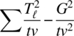 |
MSt | MSt/MSe |
| Proportionality | 1 |  |
MSf | MSf/MSe |
| Error | By subtraction | By subtraction | MSe | |
| Total | tv 2 − 1 |  |
The interested reader is referred to Bose and Stufken (2007), Bailey and Kunert (2006), and Kempton, Ferris, and David (2001) for optimality results with this proportionality assumption.
8.4 Undiminished Residual Effects Designs
The residual effects of the first order are only considered for the designs discussed in Chapters 6 and 7.
In this section, we will assume that the residual effects of each treatment are carried over to all succeeding periods undiminished. This situation arises when the treatments like surgery leave a lasting effect on the subject and the residual effect is the same for successive periods after the surgery. In small surveys, if a sensitive question is asked, the respondents’ enthusiasm may not remain the same in answering subsequent questions. Combinatorially overall balanced residual effects designs (COBREDs) provide convenient analysis for the linear model accounting for residual effects and were defined by Lakatos and Raghavarao (1987) as follows:
Definition 8.4.1 A k × b array of v treatments is said to be a COBRED if
- Every treatment occurs an equal number of times, say t, in each row.
- Every treatment occurs at most once in a column.
- Every ordered pair of symbols occurs equally often in the columns.
Note that in condition 3 of Definition 8.4.1, the ordered pair need not be only in adjacent rows as required in BRED.
This 4 × 7 array is a COBRED in 7 treatments:
| 0 | 1 | 2 | 3 | 4 | 5 | 6 |
| 1 | 2 | 3 | 4 | 5 | 6 | 0 |
| 4 | 5 | 6 | 0 | 1 | 2 | 3 |
| 6 | 0 | 1 | 2 | 3 | 4 | 5 |
Clearly, a v × v COBRED in v treatments exists if v is even, and the construction of this design will be given in Section 9.5.
Letting d(i, j) denote the treatment in the (i, j) cell as before, the linear model for these designs will be written as

The symbols will be interpreted as in Section 6.2. Under the fixed unit effects analysis, the matrices Cτ|ρ,γ,δ and Cδ|ρ,γ,τ can be seen to be circulant matrices after some extensive but routine algebra (see Lakatos, 1978).
Lakatos used these designs to estimate the residual effect, of answering a question, on the succeeding questions in a personal interview in a survey situation. To fix the ideas, let an interviewee, i, be asked four questions A, B, C, and D in the order, say, B, D, A, C. Then, denoting τA, τB, τC, τD as true responses of the questions and δA, δB, δC, δD as undiminished emotional responses carried to answering succeeding questions in the brief span of interview, the recorded responses Y1i, Y2i, Y3i, and Y4i for these four questions can be respectively modeled as
where ρ1, ρ2, ρ3, ρ4 are the ordering (or period) effects and γi is the ith interviewee effect. Questions with greater residual effects should be asked near the end of the interview rather than asking them in the beginning. Here, one can use CODWR to estimate the δ-effects. By using one of the questions as a standard bench mark, we can rank the relative questions with respect to the sensitivity of the other questions. A small survey using eight sensitive and provocative questions dealing with sex, health, and income on a student community was described by Lakatos (1978) in his thesis, where he wanted to rank the sensitive nature of these questions.
8.5 Treatment Balanced Residual Effects Designs
In many experiments, the experimenter will be interested on the simultaneous comparison of several active test treatments to a control treatment rather than all pairwise comparisons. In those circumstances, the BREDs are not necessarily optimal. Pigeon (1984) and Pigeon and Raghavarao (1987) developed CODWR useful for comparing test treatments with control such that the variances of all estimated elementary contrasts of direct and residual effects involving the control are equal and the variances between the elementary contrasts of direct effects and residual effects of treatments excluding control are equal. They showed that designs meeting this requirement are TBRED defined as follows:
8.6 A General Linear Model for CODWR
One of the main criticisms on the use of CODWR is that in most designs, they do not allow the estimation of the interaction between periods and sequences of treatments applied to the experimental units. The linear model assumed for several designs, discussed so far, does not include the interaction term. In fact, it is easy to see that due to the cross-over nature of the treatments, the estimated direct effects and residual contrasts will be confounded with the usual interaction terms of the sequences and periods.
Considering the two-period design in two sequences of Grizzle and using the notation of Chapter 7, let the data be summarized using the response means as follows:
Sequence
| (A, B) | (B, A) | |
| Period 1 | ||
| Period 2 |
Assuming that the preceding data represents a pseudo 22 factorial experiment in factors F (corresponding to rows) and G (corresponding to columns), it is easy to see that
where ![]() and
and ![]() are the estimated main effect of G and the interaction effect of F and G.
are the estimated main effect of G and the interaction effect of F and G.
If an interaction term of the sequences and periods is included in the model, then there is an overparameterization, and the direct and residual effects contrasts may not even be estimable, contrary to the purpose of the experiment. However, the significance and nonsignificance of the interaction affect the conclusions on the significance of direct and residual effects of the treatments.
One possible way appears to be to test the design as a two-way case with sequences and periods as the classifications, and if the interaction effect is not significant, proceed with the analyses described in Chapter 6 or 7. If the interaction is significant, the conclusions may be of doubtful validity.
However, one may also argue that since direct and residual effects contrasts are in the estimation space of the interaction and is a partitioning of the interaction term. As such, they can be separately tested without giving attention to the significance or nonsignificance of interaction.
Yet, another approach is to include the required interaction terms in the model paying attention not to load it. Kershner and Federer (1981) considered a general model in this respect. Modifying the notation of Chapter 6, let s sequences of treatments be used on n units where ni units receive ith sequence and let k periods be used in the experiment. Let d(i,j) be the treatment given in the ith period when jth sequence of treatments are used. Let Yiju be the observation taken on the uth unit of the jth sequence in the ith period. Then,

where μ is the general mean, ρi is the ith period effect, βj is the jth sequence effect, γj(u) is the uth unit effect in the jth sequence, τd(i,j) is the direct effect of the treatment d(i, j), δd(i–1,j) is the first-order residual effect of the treatment d(i – 1, j), ![]() is the second-order residual effect of the treatment d(i − 2, j), ρτi,d(i,j) is the interaction between the ith period and the direct effect of d(i, j), τδd(i–1,j),d(i,j) is the interaction between the direct effect of the treatment d(i, j) and the first-order residual effect of the treatment d(i − 1, j), ρδi,d(i–1,j) is the interaction between the ith period and the first-order residual effect of the treatment d(i − 1, j), and eiju are random errors distributed IIN(0, σ2); γj(u) may or may not be random effects as in Chapter 6. Let d(0, j) and d(-1, j) be considered as no treatments, and the corresponding symbols will be suppressed in the model.
is the second-order residual effect of the treatment d(i − 2, j), ρτi,d(i,j) is the interaction between the ith period and the direct effect of d(i, j), τδd(i–1,j),d(i,j) is the interaction between the direct effect of the treatment d(i, j) and the first-order residual effect of the treatment d(i − 1, j), ρδi,d(i–1,j) is the interaction between the ith period and the first-order residual effect of the treatment d(i − 1, j), and eiju are random errors distributed IIN(0, σ2); γj(u) may or may not be random effects as in Chapter 6. Let d(0, j) and d(-1, j) be considered as no treatments, and the corresponding symbols will be suppressed in the model.
The model discussed in Equation 8.6.3 is somewhat general and particular models used before are its special cases. For example, one gets CODWOR model by suppressing terms δ, δ2, ρτ, τδ, and ρδ. The CODWR model is obtained with the first-order residual effects by suppressing terms δ2, ρτ, τδ, and ρδ.
Kershner and Federer (1981) looked into fourteen two-treatment cross-over designs and concluded that the overall desirable design in the class is

a design discussed by Quenouille (1953). The design given in (8.6.4) is an F-square design as discussed in Chapter 5.
The design matrix X can be easily written for the full model (8.6.3) or a suitable submodel and analysis can be completed by using standard procedures.
8.7 Nested Design
In the case when v is large, BRED needs several units and periods, and the experimenter may not be able to conduct the study. We need a mechanism to reduce the size and time of experimentation. One possibility is to find a suitable PBCOD (m). Another possibility is to split it into two parts and use some common treatments for the two parts. Such experiments will be called nested designs. These designs were introduced by Biswas and Raghavarao (1996).
Let v1 be an even integer such that 2v1 > v and let 2v1 - v = m. Divide the treatments into three groups S1, S2, and S3 of sizes v1 - m, m, and v1 - m. Form two groups of treatments, ![]() and
and ![]() , each of size v1. Label the treatments of S2 in
, each of size v1. Label the treatments of S2 in ![]() as v1 – m + 1, v1 – m + 2, …, v1 and label the same treatments as 1, 2, …, m in
as v1 – m + 1, v1 – m + 2, …, v1 and label the same treatments as 1, 2, …, m in ![]() .
.
We will use Williams’ BRED of one Latin square for the first and second set of treatments. Using the same v1 periods and different 2v1 units, without loss of generality, the last row is marked alphabetically.
Using the notation of Chapter 6, for the experiment in v1 periods using 2v1 subjects, we have
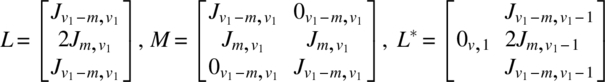
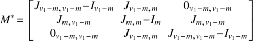

The analysis can be completed using these quantities as described in Chapter 6. It is interesting to note that if Ciτ|ρ,γ,δ is the C-matrix of τ eliminating ρ, γ, δ for the ith design (i = 1, 2) and is partitioned as

then the C-matrix for estimating τ eliminating ρ, γ, δ for the combined design is

The C-matrix for δ can be similarly obtained.
For v = 9, a BRED exists with one Latin square (see Section 9.4) needing 81 observations in 9 periods with 9 units. Using the nested design with v1 = 6, we only need 2(62) = 72 observations, saving 3 periods at the cost of adding 3 units. The following is the nested design:

8.8 Split-Plot Type CODWR
Consider the problem of treatments forming a crossed classification of two factors. Altan, McCartney, and Raghavarao (1994) considered two factors, where one factor is diazepam levels and control and the other factor is three different stimuli. Diazepam levels and control were administered to rats weekly in a crossover setting. Another crossover design was used to administer the stimuli within one day using small periods. This type of experiment indicates the need for crossover designs in a split-plot setting where one factor is administered for a longer duration and the other factor is administered for a shorter duration.
Let the treatments in a CODWR be factorial treatment combinations of two factors F1 and F2 at s1 and s2 levels, respectively. The levels of factors F1 need longer time for change, whereas levels of factor F2 can be quickly changed. CODWR in these contexts are given by Raghavarao and Xie (2003).
We form Williams’ CODWR for the levels of factor F1 in f1 periods and t1f1 units, where t1 = 1 or 2 depending on whether f1 is even or odd. We assume f1 = df2, where d is a rational number and
where t2 = 1 or 2 depending on if f2 is even or odd and α, β are positive integers. We repeat Williams’ design for the levels of factor F1, α times, so that we have αt1f1 units. Each of the whole periods will be subdivided into f2 subperiods, and a Williams’ BRED for the levels of F2 will be taken with each column in a whole period so that each treatment of the whole periods gets a multiple of the F2 level Williams’ design.With f1 = 2, f2 = 4 for the treatments (uw); u = 0, 1; w = 0, 1, 2, 3 the plan looks as follows:
| 00 | 01 | 13 | 12 | |||
| 03 | 00 | 12 | 11 | |||
| 01 | 02 | 10 | 13 | |||
| 02 | 03 | 11 | 10 | |||
| 11 | 10 | 02 | 03 | |||
| 10 | 13 | 01 | 02 | |||
| 12 | 11 | 03 | 00 | |||
| 13 | 12 | 00 | 01 | |||
For simplicity of the analysis, assume that F2 levels have no residual effects.
Let Yijℓuw be the response of the jth subperiod of the ith whole plot, ℓth unit, uth level of the whole-plot factor F1 and w is the level of the subfactor F2. Then, we take the model
where μ is the general mean; ρi is the whole period effect; ρj(i) is the jth subperiod in the ith whole period effect; γℓ is the ℓth unit effect; τd(i, ℓ) and ![]() are factors F1 and F2 levels used in the (i, ℓ) cell and (ij, ℓ) cell;
are factors F1 and F2 levels used in the (i, ℓ) cell and (ij, ℓ) cell; ![]() are the residual effects of factor F1 levels used in (i − 1, ℓ) cell with the understanding δd(0, ℓ) is identically zero; ξd(i, ℓ), d(ij, ℓ) is the interaction of direct effects of F1 level in (i, ℓ) cell and F2 level in the (ij, ℓ) cell; and eijℓ are random errors normally distributed with mean 0 and
are the residual effects of factor F1 levels used in (i − 1, ℓ) cell with the understanding δd(0, ℓ) is identically zero; ξd(i, ℓ), d(ij, ℓ) is the interaction of direct effects of F1 level in (i, ℓ) cell and F2 level in the (ij, ℓ) cell; and eijℓ are random errors normally distributed with mean 0 and ![]() ,
, ![]() for j ≠ j′. If needed, assume γℓ are random distributed IIN (0,
for j ≠ j′. If needed, assume γℓ are random distributed IIN (0, ![]() ). No interaction terms of residual effects are assumed.
). No interaction terms of residual effects are assumed.
We can verify that the whole period totals form a Williams’ design for levels of F1 factors. Then, all responses are like split-plot design except the subperiods. The subperiod within the whole period can be easily separated and analyzed for direct effects of the levels F2 and the interaction of direct effects of the levels of factors F1 and F2. The skeleton ANOVA is provided in Table 8.8.1. The SAS programming lines will be provided in Example 8.10.1.
Table 8.8.1 Skeleton ANOVA
| Source | d.f. | M.S. | F |
| Whole periods | f 1 − 1 | MSW | |
| Units | α t 1 f 1 − 1 | MSu | |
| F1 residual (el dir) | f 1 − 1 | |
|
| F1 direct (el res) | f 1 − 1 | |
|
| Error (a) | (αt1f1 − 3)(f1 − 1) | MSea | |
| Subperiods/whole period | f 1(f2 − 1) | MSS | |
| F2 direct | f 2 − 1 | |
|
| F1 × F2 direct | (f1 − 1)(f2 − 1) | MSI | MSI/MSeb |
| Error (b) | f 1(f2 − 1)(αf1t − 2) | MSeb |
The test for F1 direct and residual effects can be performed by the methods of Chapter 6 or Subsection 7.2.3. The portion below error(a) in Table 8.8.1 can be obtained after inputting the independent variables whole periods, units, subperiods, F1 levels, F2 levels, and the dependent response variable and using PROC GLM procedure using the model
response = wholefactor  units  wholefactor*units
     subperiods(wholeperiods)  subfactor  wholefactor*subfactor.
Type III sums of squares will be used to interpret the results as illustrated in the Example 8.10.1.
8.9 CODWR in Circular Arrangement
In some experimental situations, the treated units go in a circular arrangement on a belt, and a robotic arm picks up the treatment specimens for testing. In this situation, though we expect the robotic arm to be free of any residue after it collects the specimen, it is possible that some residue may be left on the arm after a specimen is collected.
Such experiments are planned by using a circular plan with v(v − 1) slots suitably numbered 1, 2, …, v(v − 1) using v treatments with v − 1 replications so that every ordered pair of distinct treatments occurs exactly once. We understand that the treatment in the v(v − 1) position leaves a residual effect on the response in the first slot. If Yi is the response from the ith slot, we assume the linear model
where μ is the general mean τi is the direct effect of the treatment in the ith slot, δi–1 is the residual effect of the (δ − 1)th slot with the understanding that δ0 = δv(v–1), and ei are IIN (0, σ2).
If Y′ = (Y1, Y2, …, Yv(v–1)), τ′ = (τ1, τ2, …, τv), δ′ = (δ1, δ2, …, δv), the normal equations are given by

where ![]() ,
, ![]() ,
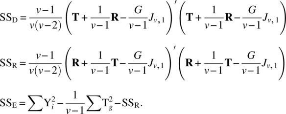
, ![]() are the least squares estimators of μ, τ, δ; G = ∑ Yi, T′ = (T1, T2, …, Tv) with Tg being the sum of responses receiving treatment g, and R′ = (R1, R2, …, Rv) with Rh being the sum of responses receiving hth treatment in the previous slot. A solution of the normal equation is
are the least squares estimators of μ, τ, δ; G = ∑ Yi, T′ = (T1, T2, …, Tv) with Tg being the sum of responses receiving treatment g, and R′ = (R1, R2, …, Rv) with Rh being the sum of responses receiving hth treatment in the previous slot. A solution of the normal equation is


Further,

Using standard methods, the ANOVA Table 8.9.1 can be obtained.
Table 8.9.1 ANOVA table for circular residual effects design
| Source | d.f. | S.S. | M.S. | F |
| Direct (ig res) | v − 1 | 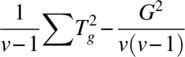 |
||
| Residual (el dir) | v − 1 | SSR | MSR | MSR/MSe |
| Direct (el res) | v − 1 | SSD | MSD | MSD/MSe |
| Error | v 2 − 3v + 1 | SSE | MSe | |
| Total | v(v − 1) − 1 |  |
||
 |
||||
A numerical example will be given in Example 8.10.2. It may be noted that the nonorthogonality between the direct and residual effects will be eliminated by taking all identical pairs of treatments once.
8.10 Numerical Examples
We will now provide two examples illustrating the analysis for the designs discussed in Sections 8.8 and 8.9.
Table 8.10.1 Artificial data on exercise time, medication, and run times
| Aα(100) | Aβ(93) | Bγ(110) | Bδ(105) | ||||||
| Aδ(95) | Aα(99) | Bβ(107) | Bγ(107) | ||||||
| Aβ(105) | Aγ(95) | Bδ(109) | Bα(108) | ||||||
| Aγ(97) | Aδ(98) | Bα(110) | Bβ(109) | ||||||
| Bβ(110) | Bα(107) | Aδ (99) | Aγ(100) | ||||||
| Bα(108) | Bβ(109) | Aγ (98) | Aβ(100) | ||||||
| Bγ (103) | Bδ(106) | Aα(97) | Aδ (97) | ||||||
| Bδ(104) | Bγ(107) | Aβ(99) | Aα(96) |
The programming lines accounting direct and residual effects of medications, direct effect of exercise, and interaction of direct effects of medication and exercise is given as follows along with the output:
data a;
input unit wholeperiod subperiod wholefactor subfactor response @@;cards;
1 1 1 1 1 100 1 1 2 1 2 95 1 1 3 1 3 105 1 1 4 1 4 97
2 1 1 1 3 93 2 1 2 1 1 99 2 1 3 1 4 95 2 1 4 1 2 98
3 1 1 2 4 110 3 1 2 2 3 107 3 1 3 2 1 109 3 1 4 2 2 110
4 1 1 2 2 105 4 1 2 2 4 107 4 1 3 2 1 108 4 1 4 2 3 109
1 2 5 2 3 110 1 2 6 2 1 108 1 2 7 2 4 103 1 2 8 2 2 104
2 2 5 2 1 107 2 2 6 2 3 109 2 2 7 2 2 106 2 2 8 2 4 107
3 2 5 1 2 99 3 2 6 1 4 98 3 2 7 1 1 97 3 2 8 1 4 99
4 2 5 1 1 100 4 2 6 1 2 100 4 2 7 1 3 97 4 2 8 1 4 96
;
data b;set a; proc sort;by unit;
proc univariate noprint;
var response;
output out = b1 sum = sum ;by unit;

data b1;set b1;
if unit in(1,2) then group = 1;
else group = 2;
proc ttest;var sum;

class group;run;
data c1;set a;
if wholeperiod = 1; response1 = response; keep unit response1;proc sort;by unit;
data c2;set a;
if wholeperiod = 2;
response2 = response;
keep unit response2; proc sort;by unit;

data c;merge c1 c2;by unit;
responsediff = response1-response2;

proc univariate noprint;
var responsediff;
output out = cc sum = sum ;by unit;

data cc;set cc;
if unit in(1,2) then group = 1;
else group = 2;
proc ttest;var sum;
class group;run;

data a;set a;
proc glm data = a;
class unit wholeperiod subperiod wholefactor subfactor;
model response = unit wholefactor unit*wholefactor subperiod(wholeperiod)
subfactor wholefactor*subfactor; run;| The TTEST Procedure | ||||||||
| Variable: sum (the sum, response) | ||||||||
| group | N | Mean | Std Dev | Std Err | Minimum | Maximum | ||
| 1 | 2 | 818.0 | 5.6569 | 4.0000 | 814.0 | 822.0 | ||
| 2 | 2 | 825.5 | 4.9497 | 3.5000 | 822.0 | 829.0 | ||
| Diff(1-2) | −7.5000 | 5.3151 | 5.3151 | |||||
| group | Method | Mean | 95% CL | Mean | Std Dev | 95% CL | Std Dev |
| 1 | 818.0 | 767.2 | 868.8 | 5.6569 | 2.5238 | 180.5 | |
| 2 | 825.5 | 781.0 | 870.0 | 4.9497 | 2.2083 | 157.9 | |
| Diff(1-2) | Pooled | −7.5000 | −30.3689 | 15.3689 | 5.3151 | 2.7673 | 33.4038 |
| Diff(1-2) | Satterthwaite | −7.5000 | −30.7594 | 15.75 |
| Method | Variances | DF | t Value | Pr > |t| |
| Pooled | Equal | 2 | −1.41 | 0.2937(a2) |
| Satterthwaite | Unequal | 1.9654 | −1.41 | 0.2957(a3) |
| Equality of Variances | ||||||||
| Method | Num DF | Den DF | F Value | Pr > F | ||||
| Folded F | 1 | 1 | 1.31 | 0.9152(a1) | ||||
| The TTEST Procedure | ||||||
| Variable: sum (the sum, responsediff) | ||||||
| group | N | Mean | Std Dev | Std Err | Minimum | Maximum |
| 1 | 2 | −36.0000 | 11.3137 | 8.0000 | −44.0000 | −28.0000 |
| 2 | 2 | 39.5000 | 4.9497 | 3.5000 | 36.0000 | 43.0000 |
| Diff(1-2) | −75.5000 | 8.7321 | 8.7321 | |||
| group | Method | Mean | 95% CL | Mean | Std Dev | 95% CL | Std Dev |
| 1 | −36.0000 | −137.6 | 65.6496 | 11.3137 | 5.0476 | 361.0 | |
| 2 | 39.5000 | −4.9717 | 83.9717 | 4.9497 | 2.2083 | 157.9 | |
| Diff (1-2) | Pooled | −75.5000 | −113.1 | −37.9287 | 8.7321 | 4.5465 | 54.8791 |
| Diff (1-2) | Satterthwaite | −75.5000 | −135.7 | −15.3290 |
| Method | Variances | DF | t Value | Pr > |t| |
| Pooled | Equal | 2 | −8.65 | 0.0131 (a5) |
| Satterthwaite | Unequal | 1.3693 | −8.65 | 0.0368 (a6) |
| Equality of Variances | ||||||||
| Method | Num DF | Den DF | F Value | Pr > F | ||||
| Folded F | 1 | 1 | 5.22 | 0.5251 (a4) | ||||
***
| The GLM Procedure | |||||
| Dependent Variable: response | |||||
| Source | DF | Sum of Squares | Mean Square | F Value | Pr > F |
| Model | 19 | 837.2014299 | 44.0632332 | 9.23 | 0.0002 |
| Error | 12 | 57.2673201 | 4.7722767 | ||
| Corrected Total | 31 894.4687500 | ||||
| R-Square | Coeff Var | Root MSE | response Mean |
| 0.935976 | 2.126734 | 2.184554 | 102.7188 |
***
| Source | DF | Type III SS | Mean Square | F Value | Pr > F |
| unit | 3 | 21.2522186 | 7.0840729 | 1.48 | 0.2685 |
| wholefactor | 1 | 659.9255195 | 659.9255195 | 138.28 | < .0001 |
| unit*wholefactor | 2 | 16.5900248 | 8.2950124 | 1.74 | 0.2173 |
| subperiod(wholeperi) | 6 | 63.8136984 | 10.6356164 | 2.23 | 0.1119 |
| subfactor | 3 | 11.4342090 | 3.8114030 | 0.80 | 0.5181 (a7) |
| wholefacto*subfactor | 3 | 30.8698723 | 10.2899574 | 2.16 | 0.1463 (a8) |
The p-value at (a1) is used to test the significance of the equality of the variances to test the significances of δA = δB. If this is significant, the p-value given at (a3) will be used to test δA = δB, and the p-value given at (a2) to test the significance if (a1) is not significant. In our example, the p-value at (a1) is not significant, and hence, using (a2), we conclude that δA = δB.
The p-value at (a4) is used to test the significance of the equality of the variances for testing τA = τB. If this is significant, the p-value given at (a6) will be used to test τA = τB, and the p-value given at (a5) to test the significance if (a4) is not significant. In our example, the p-value at (a4) is not significant, and hence, using (a5), we conclude that τA ≠ τB.
The p-value at (a8) is used to test the significance of the direct effects of whole and subfactors. In our example, this is not significant. The p-value at (a7) will be used to test the significance of the direct effects of the subfactor. In this example, this is not significant.
Table 8.10.2 Artificial data of a testing experiment
| Drink | A | D | B | C | B | D | A | C | D | C | A | B |
| Rating | 4 | 3 | 5 | 2 | 3 | 4 | 6 | 2 | 5 | 7 | 2 | 2 |
The programming lines and output are given as follows:
data a ; input direct residual response @@;cards;
1 2 4 4 1 3 2 4 5 3 2 2 2 3 3 4 2 4 1 4 6 3 1 2 4 3 5 3 4 7 1 3 2 2 1 2
;
proc glm data = a;
class direct residual;
model response = direct residual;
contrast 'direct' direct 1 -1 0 0 ;
contrast 'residual' residual 1 -1 0 0 ; run;
***
| The GLM Procedure | |||||
| Dependent Variable: response | |||||
| Source | DF | Sum of Squares | Mean Square | F Value | Pr > F |
| Model | 6 | 27.00000000 | 4.50000000 | 4.29 | 0.0659 |
| Error | 5 | 5.25000000 | 1.05000000 | ||
| Corrected Total | 11 | 32.25000000 | |||
| R-Square | Coeff Var | Root MSE | response Mean |
| 0.837209 | 27.32520 | 1.024695 | 3.750000 |
***
| Source | DF | Type III SS | Mean Square | F Value | Pr > F |
| direct | 3 | 4.75000000 | 1.58333333 | 1.51 | 0.3204 (b1) |
| residual | 3 | 26.08333333 | 8.69444444 | 8.28 | 0.0220 (b2) |
| Contrast | DF | Contrast SS | Mean Square | F Value | Pr > F |
| direct | 1 | 0.18750000 | 0.18750000 | 0.18 | 0.6902 (b3) |
| residual | 1 | 1.02083333 | 1.02083333 | 0.97 | 0.3694 (b4) |
The p-values given at (b1) and (b2) of the output are used for testing the equality of the direct and residual effects of all the treatments. In our example, the residual effects of all treatments are different, whereas the direct effects are not significant. The p-value given at (b3) can be used for testing the direct effects contrast of τA - τB and is not significant in our example. The p-value given at (b4) is used to test the residual effects contrast of δA - δB and is not significant in our example.
References
- Altan S, McCartney M, Raghavarao D. Two methods of analysis for a complex behavioral experiment. J Biopharm Statist 1994;4:437–447.
- Bailey RA, Kunert J. On optimal crossover designs when carryover effects are proportional to direct effects. Biometrika 2006;93:613–625.
- Bechhofer RE, Tamhane AC. Incomplete block designs for comparing treatment with a control: general theory. Technometrics 1981;23:45–57.
- Biswas N, Raghavarao D. Nested residual effect design. Sankhya 1996;58:240–244.
- Bose M, Stufken J. Optimal crossover designs when carry over effects are proportional to direct effects. J Statist Plan Inf 2007;137:3291–3302.
- Dean AM, Lewis SM, Chang JY. Nested changeover designs. J Statist Plan Inf 1999;77:337–351.
- Dunnett CW. A multiple comparison procedure for comparing several treatments with a control. Am Statist Assoc 1955;50:1096–1121.
- Hedayat AS, Yang M. Optimal and efficient crossover designs for comparing test treatments with a control treatment. Ann Math Statist 2005;33:915–943.
- Kempton RA, Ferris SJ, David O. Optimal change-over designs when carry-over effects are proportional to direct effects of treatments. Biometrika 2001;88:391–399.
- Kershner R, Federer WT. Two-treatment cross-over designs for estimating a variety of effects. J Am Statist Assoc 1981;76:612–619.
- Lakatos E. Undiminished residual effects designs and their applications to survey sampling [Unpublished Ph.D. dissertation]. College Park, MD: University of Maryland.
- Lakatos E, Raghavarao D. Undiminished residual effect designs and their applications. Comm Statist – Theor Meth 1987;16:1345–1359.
- Lucas HL. Extra-period Latin square change-over design. J Dairy Sci 1957;40:225–239.
- Majumdar D. Optimal and efficient treatment-control designs. In: Ghosh S, Rao R, editors. Handbook of Statistics, vol. 13. Amsterdam: Elsevier; 1996. p 1007–1053.
- Majumdar D. Optimal repeated measurements designs for comparing test treatments with a control. Comm Statist—Theor Meth 1988;17:3687–3703.
- Pigeon JG. Residual effects designs for comparing treatments with a control. [Unpublished Ph.D. dissertation]. Philadelphia, PA: Temple University; 1984.
- Pigeon JG, Raghavarao D. Cross-over designs for comparing treatments with a control. Biometrika 1987;74:321–328.
- Quenouille MH. The Design and Analysis of Experiments. London: Charles Griffin and Company, Ltd; 1953.
- Raghavarao D, Xie YC. Split-plot type cross-over designs. J Statist Plan Inf 2003;116:197–207.