
Chapter 6
Cross-Over Designs with Residual Effects
6.1 INTRODUCTION
In Chapter 1 and Section 5.1, it was indicated that when a sequence of treatments are applied on an experimental unit over several periods and if no washout period can be left between successive periods, the analysis of the design has to be carried by taking into account the residual effects in the assumed linear model. It was further indicated that the direct effect of the treatment is the effect of the treatment manifested in the period of its application and ith-order residual effect is the residual effect of the treatment in the ith period after the treatment’s application is discontinued. While it is possible that the residual effects of all orders may be the same and this will be discussed in Section 8.2, in most designs, the residual effects of second and higher orders will be negligible and cross-over designs with first-order residual effects (CODWR) will be discussed in this chapter.
Since the treatments are applied to the experimental units without a break in CODWR, it becomes desirable to make allowance for a unit to be untreated in some periods. In the most general case of CODWR, one can consider b experimental units used over a k period experiment where in each period a unit may or may not receive one of the v treatments 1, 2, …, v. The setting can be written as a k × b array using v treatments. Let N = (nij) be a k × b matrix where nij = 1 or 0 according as the jth unit receives a treatment or not in the ith period. If nij = 1, let d(i, j) denote the treatment applied to the jth unit in the ith period. Mercado (1976) noted that observations may be taken in the ith period on the jth unit whether or not that unit receives a treatment in the period under consideration, and he classified the designs as generalized residual effects designs-I (GRED-I), if the observations are taken on the units only in the periods with nij = 1, and as generalized residual effects designs-II (GRED-II), if the observations are taken in all periods on each unit.
The analysis of GRED-I will be discussed in Section 6.2 and will be specialized to the case when N = Jk,b. We will also briefly sketch the analysis of GRED-II designs and indicate the estimability of direct and residual effects in that section. The designs will then be characterized as BRED and partially balanced cross-over designs with m associate classes (PBCOD(m)) depending on the incidence structure of the treatments in the rows and columns of the designs in Sections 6.3 and 6.4. Numerical examples will be given in Section 6.5. The analysis when units are random will be given in Section 6.6. Finally, some concluding remarks will be given in Section 6.7.
6.2 Analysis of CODWR
Consider a GRED in a k × b array using v treatments and let N = (nij) be the k × b matrix indicating the pattern of treating or not treating a unit in a particular period. When nij = 1, let Yij be the observation recorded in the ith period on the jth unit for GRED-I. Let
where μ is the general mean; ρi is the ith period effect; γj is the jth unit effect; τd(i, j) is the direct effect of treatment d(i, j), the treatment applied on the jth unit in the ith period; δd(i–1, j) is the first-order residual effect of the treatment d(i – 1, j); and eij are random errors distributed according to IIN (0, σ2). When there is no treatment in the cell (i – 1, j), we take δd(i–1, j) = 0. Clearly, δd(0, j) = 0.
Let ![]() be the direct effects-periods, direct effects-units, residual effects-periods, residual effects-units, and direct effects-residual effects incidence matrices, respectively.
be the direct effects-periods, direct effects-units, residual effects-periods, residual effects-units, and direct effects-residual effects incidence matrices, respectively.
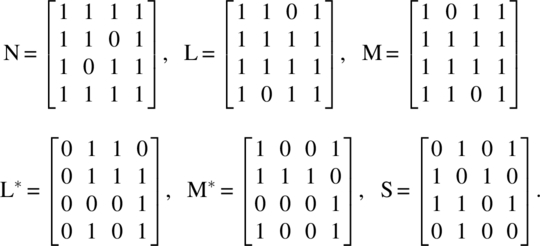
For the CODWR,
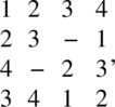
where “–” denotes an untreated cell, the matrices N, L, M, L*, M*, and S are, respectively, given by
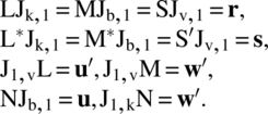
Let ui be the number of units observed during the ith period, wj be the number of periods in which the jth unit is observed, rg be the number of observations on cells receiving the gth treatment, and sh be the number of cells observed preceded by cells receiving the hth treatment. Let u′ = (u1, u2, …, uk), w′ = (w1, w2, …, wb), r′ = (r1, r2, …, rv), and s′ = (s1, s2, …, sv). The following relations are then obvious:
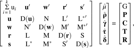
Let G be the grand total of all observations, Pi be the total of observations in the ith period, Cj be the total of observations on the jth unit, Tg be the total of observations in which the gth treatment occurs, and Rh be the total of observations in which the residual effect of the hth treatment occurs. Let P′ = (P1, P2, …, Pk), C′ = (C1, C2, …, Cb), T′ = (T1, T2, …, Tv), R′ = (R1, R2, …, Rv), ρ′ = (ρ1, ρ2, …, ρk), γ′ = (γ1, γ2, …, γb), τ′ = (τ1, τ2, …, τv), and δ′ = (δ1, δ2, …, δv). The normal equations can then be easily verified to be
where ![]() ,
, ![]() ,
, ![]() ,
, ![]() , and
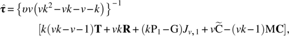
, and ![]() are the least squares estimators of μ, ρ, γ, τ, and δ, respectively. Note that we are using C as a column vector and it is not a C-matrix. Continuing the notation of Cα|β,γ,… as introduced in the last chapter, the reduced normal equations after eliminating
are the least squares estimators of μ, ρ, γ, τ, and δ, respectively. Note that we are using C as a column vector and it is not a C-matrix. Continuing the notation of Cα|β,γ,… as introduced in the last chapter, the reduced normal equations after eliminating ![]() ,
, ![]() , and
, and ![]() are
are
where
and
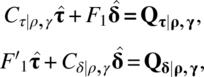
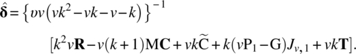
The reduced normal equations for estimating ![]() and
and ![]() from Equation (6.2.4) after eliminating
from Equation (6.2.4) after eliminating ![]() and
and ![]() are, respectively,
are, respectively,
and
where
and
The ANOVA table is then given in Table 6.2.1. Tests of significance and confidence intervals on the contrasts of direct effects as well as residual effects of the treatments can then be made by standard procedures. The detailed results will be discussed for BRED in Section 6.3.
Table 6.2.1 ANOVA for GRED-I
| Source | d.f. | S.S. | M.S. | F |
| Periods (ig units, direct and residual effects) | k – 1 | 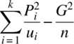 |
||
| Units | ||||
| (el periods, ig direct and residual effects) | R(Cγ|ρ) | Q |
||
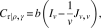
| Direct effects | ||||
| (el periods and units, ig residual effects) | R(Cτ|ρ,γ) | Q |
||
| Residual effects | ||||
| (el periods, units, direct effects) | R(Cδ|ρ,γ,τ) | Q |
MSr | MSr/MSe |
| Direct effects | ||||
| (el periods, units, and residual effects) | R(Cτ|ρ,γ,δ) | |
MSd | MSd/MSe |
| Error SSe | υ* | SSe | MSe | |
| Total | n – 1 |  |
Qγ|ρ = C – N′{D(u)}-1P, SSe = total SS – period SS – unit SS – dir. eff. (ig res. eff.) SS – res. eff. SS, n = ![]() , υ* = (n – 1)–{(k – 1) + R(Cγ|ρ) + R(Cτ|ρ,γ) + R(Cδ|ρ,γ,τ)}, ∑+ denotes summation over all treated cells, and R(⋅) denotes the rank of the matrix in parenthesis.
, υ* = (n – 1)–{(k – 1) + R(Cγ|ρ) + R(Cτ|ρ,γ) + R(Cδ|ρ,γ,τ)}, ∑+ denotes summation over all treated cells, and R(⋅) denotes the rank of the matrix in parenthesis.
The equality of direct effects as well as residual effects will be tested by using the F statistics of Table 6.2.1 in the usual way. Most of the CODWR discussed in the literature have N = Jk,b, and every treatment occurs t times in each row of the design so that L = tJv,k and b = tv. Such designs will hence worth be called regular CODWR. Such designs are also called uniform designs across periods. Designs with k, a multiple of v, and every treatment occurs equally often in the columns are called uniform designs across units. A design is uniform if it is uniform in periods and units.
Clearly, for a regular CODWR, we get
and
From Equations (6.2.13), (6.2.14), (6.2.17), (6.2.18), and (6.2.19), it is clear that if MM*′ is expressed in terms of MM′ and M* M*′, the dispersion matrices of direct and residual effects will be functions of MM′, M* M*′, and S, and it is easy to obtain their structures from the structures of MM′, M* M*′, and S. To this end, the following lemma is useful:
Regular CODWR satisfying the requirements of Lemma 6.2.1 can be characterized as BRED and PBCOD(m) based on MM′, M* M*′, and S. These results will be discussed in Sections 6.3 and 6.4.
For GRED-II, observations will be taken in treated and untreated cells. The model for the response from an untreated cell will contain the period and unit effects parameters and will not contain direct effects parameters. If the unit is treated preceding the untreated cell, then the model also contains the residual effects parameters. Here, N = Jk,b, L, M, and S will be the same as earlier, but L*, M* matrices will be different. The C-matrices and ANOVA table will be the same as GRED-I.
Noting that a linear parameter function ![]() is estimable for a linear model,
is estimable for a linear model,
iff
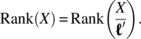
It can be verified that for all CODWR designs, the linear parametric contrast ρ1 - ρj is not estimable, whereas all other contrasts ρi - ρj are estimable for j = 1, 2, 3, …, k; 2 ≤ i < j.
Consider a CODWR
If all 16 observations are nonmissing, then Rank(Cτ|ρ,γ,δ) = Rank(Cδ|ρ,γ,τ) = 3 and all independent contrasts of treatment effects as well as residual effects are estimable.
Suppose the observation on unit 1 is missing in the first period. As GRED-I, Rank(Cδ|ρ,γ,τ) = 4 and Rank(Cτ|ρ,γ,δ) = 3, indicating that all contrasts of direct effects are estimable and all individual residual effects parameters are estimable. If the design is considered as GRED-II, then Rank(Cτ|ρ,γ,δ) = Rank(Cδ|ρ,γ,τ) = 4 and all individual direct effects and residual effects parameters are estimable. This result is true in general for the residual effects when the missing observation is not in the last period and is always true for direct effects parameters for GRED-II. An intuitive justification for the phenomenon is that we assume the empty cell is providing a carryover effect δ0, which is identically zero, and as a GRED-II, it produces τ0, which is identically zero. Since all contrasts are estimable, δi - δ0 ≡ δi, τi - τ0 ≡ τi are estimable.
Another interesting observation of Mercado (1976) is that for the design (6.2.26), if two cells (1, 1) and (2, 2) are missing, then individual δi are nonestimable and only contrasts δi - δj are estimable. If cells (1, 1) and (2, 3) are missing, all individual δi′s are estimable. The estimation of linear parametric functions of τi and δi for any GRED-I and/or GRED-II is an interesting and challenging problem.
6.3 Bred
If MM′, M* M*′, S, and MM*′ are completely symmetric matrices, then Cτ|ρ,γ, Cδ|ρ,γ, and F1 are completely symmetric and it follows that Cτ|ρ,γ,δ, Cδ|ρ,γ,τ are completely symmetric. In that case, the design is variance balanced in the estimation of the contrasts of direct effects as well as residual effects of the treatments.
In view of Lemma 6.2.1 under the condition stated there, it is sufficient that MM′, M* M*′, and S are completely symmetric in order that Cτ|ρ,γ,δ and Cδ|ρ,γ,τ be completely symmetric and the design is variance balanced for the estimation of the contrasts of direct effects as well as residual effects of the treatments. MM′ is completely symmetric if M is the incidence matrix of a BIBD discussed in Section 5.6, and thus, the b columns of the residual effects design form a BIBD of block size k. M* M*′ is completely symmetric if M* is the incidence matrix of a BIBD and thus the b columns of the residual effects design omitting the last row form a BIBD of block size k − 1. Finally, S will be completely symmetric if every ordered pair of treatments (i, j), for i ≠ j, occurs together in successive rows equally often, say, υ times. These considerations lead us to the following definition:
- Every column contains distinct treatments.
- Every treatment occurs t times in each row.
- For every pair of distinct treatments i and j, the number of columns in which i occurs with j in the last row is the same as the number of columns in which j occurs with i in the last row.
- The b columns form a BIBD with parameters v1 = v, b1 = b, r1 = tk, k1 = k, λ1 = λ.
- The b columns excluding the last row form a BIBD with parameters v2 = v, b2 = b, r2 = t (k − 1), k2 = k − 1, λ2 = μ.
- For every pair of distinct treatments i and j, the number of columns in which the ordered pair of treatments (i, j) occurs in successive rows is υ.
The parameters of a BRED are v, k, b, t, λ, μ, and υ, and they satisfy the following relations:

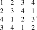
The design

can be easily verified to be a BRED with parameters v = 4 = b = k, t = 1, λ = 4, μ = 2, and υ = 1. The design

can be seen to be a BRED with parameters v = 3 = k, b = 6, t = 2, λ = 6, μ = 2, and υ = 2.
These two examples have a complete replication of all treatments in the columns. Williams (1949) showed that a BRED can always be constructed with one or two Latin squares depending on whether v is even or odd, and the construction methods will be given in Section 9.4.
Patterson (1952) gave BREDs where k < v, and some of his construction methods will be discussed in Section 9.5. An example of a BRED with v = 7, b = 14, k = 4, t = 2, r = 8, λ = 4, μ = 2, and υ = 1 is
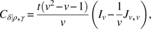
From Definition 6.3.1 and Lemma 6.2.1, we get

and
Thus, for the BRED, Equations (6.2.13) and (6.2.14) simplify to

and

To get the vectors of adjusted yield, let ![]() be the sum of the column totals where treatment i is in the last row and put
be the sum of the column totals where treatment i is in the last row and put ![]() . After some simplification, one gets
. After some simplification, one gets

Thus,
and
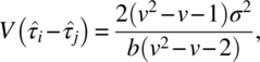
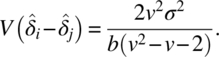
Clearly,

and

These variances indicate that ![]() i –
i – ![]() j is estimated more accurately than
j is estimated more accurately than ![]() i –
i – ![]() j. The ANOVA table given in 6.2.1 can be easily completed to test the significance of direct effects as well as residual effects of the treatments.
j. The ANOVA table given in 6.2.1 can be easily completed to test the significance of direct effects as well as residual effects of the treatments.
For Williams’ BREDs consisting of one or two Latin squares, MC = GJv,1 and
and
The ANOVA table for these designs is given in Table 6.3.1.
Here,
and
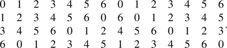
In the literature, strongly balanced residual effects are considered where every treatment precedes itself on units the same number of times it precedes other treatments. With v = 4 treatments, k = 8 periods, and b = 16 units, the following design is uniform on both periods and units and is strongly balanced as every pair of treatments occurs four times in successive periods:

There is a vast literature on the optimality of BRED for estimating direct effects and residual effects contrasts considering different classes of competing designs, and the interested reader is referred to Bose and Dey (2009), Cheng and Wu (1980), Hedayat and Afsarinejad (1975, 1978), Hedayat and Yang (2003, 2004), Kunert (1983, 1984), Kushner (1997, 1998, 1999), Laska, Meisner, and Kushner (1983), Shah, Bose, and Raghavarao (2005), and Stufken (1996).
Table 6.3.1 ANOVA table for BREDs of Williams
| Source | d.f. | S.S. | M.S. | F |
| Periods | v – 1 | 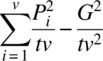 |
||
| Units | tv – 1 |  |
||
| Direct effects (ig residual effects) | v – 1 |  |
||
| Residual effects (el direct effects) | v – 1 | 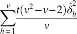 |
MSr | MSr/MSe |
| Direct effects (el residual effects) | v – 1 |  |
MSd | MSd/MSe |
| Error | (v – 1) (tv – 3) | a+ | MSe | |
| Total | tv 2 – 1 | 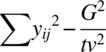 |
a+ = total SS – period SS – units SS – direct effects (ig res. eff.) SS – residual effects (el dir. eff.) SS.
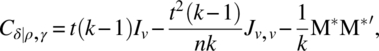
We will conclude this section by giving a simple result on optimality. In a class of designs, a design is optimal for all optimality criterion, that is, universal optimal, for the estimation of the effects of a factor, if the C-matrix for estimating these effects eliminating all other factors is completely symmetric with maximum trace. In the class of uniform CODWR with k = v, b = tv, N = Jk,b, without loss of generality, assume that the last period has treatments 1, 2, …, v occurring in that order t times. Then, we verify
and hence, the trace of Cτ|ρ,γ,δ and Cδ|ρ,γ,τ is maximum iff ![]() is minimum. Since ∑ i ≠ jsij = t(v − 1)v,
is minimum. Since ∑ i ≠ jsij = t(v − 1)v, ![]() is minimum iff sij is constant for i ≠ j, and those designs are Williams’ BRED.
is minimum iff sij is constant for i ≠ j, and those designs are Williams’ BRED.
6.4 PBCOD (m)
PBCOD (m) were introduced by Blaisdell and Raghavarao (1980) generalizing the concept of BRED in which there are m types of variances for the estimated elementary contrasts of direct effects as well as residual effects of treatments. For defining these designs, the concepts of association scheme and partially balanced incomplete block design (PBIBD) are required and are introduced in the following definitions:
Given an association scheme, we define m, v × v matrices ![]() for i = 1, 2, …, m, where
for i = 1, 2, …, m, where
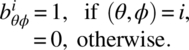
In addition, put B0 = Iv ⋅ B0, B1, …, Bm are known as the association matrices of the m-class association scheme, and they satisfy the relations

where ![]() being the Kronecker delta equal to 1 if i = j and 0 otherwise. From Equation (6.4.2), clearly, matrix multiplication is closed in the set of linear functions of B0, B1, …, Bm, and the regular or (g-inverse) of a linear function of B0, B1, …, Bm is again a linear function of the association matrices.
being the Kronecker delta equal to 1 if i = j and 0 otherwise. From Equation (6.4.2), clearly, matrix multiplication is closed in the set of linear functions of B0, B1, …, Bm, and the regular or (g-inverse) of a linear function of B0, B1, …, Bm is again a linear function of the association matrices.
Using an association scheme, we define a PBIBD in Definition 6.4.2:
Although the analysis of these designs is quite straightforward, the algebra is rather tedious and lengthy and will not be presented here. It depends in expressing all involved matrices in terms of linear combinations of the association matrices and defining the g-inverse of ![]() , where ∑ aiBiJv,1 = 0v,1, as
, where ∑ aiBiJv,1 = 0v,1, as ![]() , satisfying
, satisfying
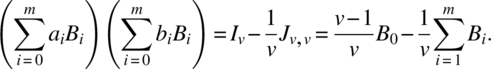
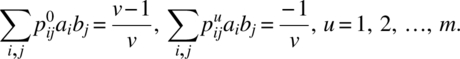
We solve the following simultaneous equations to determine b0, b1, …, bm:
Defining the efficiency, Ed (or Er) of PBCOD (m) as a/kt where 2σ2/a is the average variance of the elementary contrasts of direct (or residual) treatment effects, Raghavarao and Blaisdell (1985) proved the following:
This section will be concluded with the note that there is a need of developing efficient PBCOD (m) to increase the bag of CODWR to meet all requirements of experimenters in this area.
6.5 Numerical Example
The SAS program for analyzing a CODWR will be illustrated with the following BRED example. In the program, we denote Qγ|ρ, Qτ|ρ,γ, Qδ|ρ,γ, Qτ|ρ,γ,δ, and Qδ|ρ,γ,τ by Q1, Q2, Q3, Q4, and Q5, respectively. Further, Cγ|ρ, Cτ|ρ,γ, Cδ|ρ,γ, Cτ|ρ,γ,δ, and Cδ|ρ,γ,τ will be denoted by C1, C2, C3, C4, and C5, respectively. The symbols T, R, r, s, L*, and M* will be denoted as trt, rtrt, smallr, smalls, lstar, and mstar, respectively.
Table 6.5.1 Apples sale data using a three-period BRED
| Period | Store | Total | |||||
| 1 | 2 | 3 | 4 | 5 | 6 | ||
| I | A(720) | B(1020) | C(640) | A(1640) | B(2080) | C(960) | 7060 |
| II | B(900) | C(820) | A(720) | C(1560) | A(1560) | B(1120) | 6680 |
| III | C(720) | A(920) | B(800) | B(2090) | C(1784) | A(900) | 7214 |
| Total | 2340 | 2760 | 2160 | 5290 | 5424 | 2980 | 20,954 |
The following SAS program provides the necessary output.
data a; input row column dirtrt$ restrt$ response @@; cards;
1 1 A . 720 1 2 B . 1020 1 3 C . 640 1 4 A . 1640 1 5 B . 2080 1 6 C . 960
2 1 B A 900 2 2 C B 820 2 3 A C 720 2 4 C A 1560 2 5 A B 1560 2 6 B C 1120
3 1 C B 720 3 2 A C 920 3 3 B A 800 3 4 B C 2090 3 5 C A 1784 3 6 A B 900
;
data row;set a;proc sort;by row;
proc univariate noprint; var response; output
out=rowsum sum=p;by row;
data rowsum;set rowsum;
data column;set a;proc sort;by column;
proc univariate noprint; var response; output
out=colsum sum=c;by column;
data colsum;set colsum;
data dirtrt;set a;proc sort;by dirtrt;
proc univariate noprint; var response; output
out=dirtrtsum sum=trt;by dirtrt;
data dirtrtsum;set dirtrtsum;
data restrt;set a;proc sort;by restrt;
proc univariate noprint; var response; output
out=restrtsum sum=rtrt;by restrt;
data restrtsum;set restrtsum;if restrt= ' ' then delete;
data grandtotal;set a;
proc univariate noprint; var response; output
out=grandtotal sum=grandtotal n=grandn;
data grandtotal;set grandtotal;
data sqobs;set a;responsesq=response*response;
proc univariate noprint; var responsesq; output
out=responsesq sum=respsq;
data responsesq;set responsesq;
proc iml;
/*****input data***/
n=J(3,6,1);l=J(3,3,2);m=j(3,6,1);lstar=shape({0 2 2},3,3);
mstar={1 0 1 1 1 0,1 1 0 0 1 1, 0 1 1 1 0 1};
s={0 2 2, 2 0 2, 2 2 0};u=J(3,1,6); w=J(6,1,3);
smallr=J(3,1,6);smalls=J(3,1,4);k=3;*number of rows in the design;
treatment={1,2,3};
/***end of data input***/
use rowsum;read all var {p} into p ; use colsum;read all var {c} into c ;
use dirtrtsum;read all var {trt} into trt ; use restrtsum;read all var {rtrt} into rtrt ;
use grandtotal;read all var {grandtotal} into grandtotal ;
use grandtotal;read all var {grandn} into grandn ;
use responsesq;read all var {respsq} into respsq ;
q1=c-n`*inv(diag(u))*p;
c1=diag(w)-n`*inv(diag(u))*n;
c2=diag(smallr)-l*inv(diag(u))*l`-(m-l*inv(diag(u))*n)*ginv(c1)*(m-l*inv(diag(u))*n)`;
q2=trt-l*inv(diag(u))*p-(m-l*inv(diag(u))*n)*ginv(c1)*(c-n`*inv(diag(u))*p);
c3=diag(smalls)-lstar*inv(diag(u))*lstar`-(mstar-lstar*inv(diag(u))*n)*ginv(c1)*(mstar-lstar*inv(diag(u))*n)`;
q3=rtrt-lstar*inv(diag(u))*p-(mstar-lstar*inv(diag(u))*n)*ginv(c1)*
(c-n`*inv(diag(u))*p);
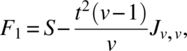
f1=s-l*inv(diag(u))*lstar`-(m-l*inv(diag(u))*n)*ginv(c1)*(mstar-lstar*inv(diag(u))*n)`;
c4=c2-f1*ginv(c3)*f1`; q4=q2-f1*ginv(c3)*q3;
c5=c3-f1`*ginv(c2)*f1; q5=q3-f1`*ginv(c2)*q2;
periodss= (p`*inv(diag(u))*p)-(grandtotal**2)/grandn;
unitss=(q1`*ginv(c1)*q1); unitdf=round(trace(ginv(c1)*c1));
dirigresss=q2`*ginv(c2)*q2; dirigresdf=round(trace(ginv(c2)*c2));
reseldirss=q5`*ginv(c5)*q5; reseldirdf=round(trace(ginv(c5)*c5));
direlresss=q4`*ginv(c4)*q4; direlresdf=round(trace(ginv(c2)*c4));
totalss=respsq-grandtotal**2/grandn;
errorss=totalss-periodss-unitss-dirigresss-reseldirss;
error_df=grandn-1-(k-1)-unitdf-dirigresdf-reseldirdf;
error_ms=errorss/error_df;
direlresms=direlresss/direlresdf;
reseldirms=reseldirss/reseldirdf;
reseldirf=reseldirms/(errorss/error_df);
direlresf=direlresms/(errorss/error_df);direct_pvalue=1-probf(direlresf,direlresdf,error_df);residual_pvalue=1-probf(reseldirf,reseldirdf,error_df);
direct=ginv(c4)*q4; residual=ginv(c5)*q5;
ginvc4=ginv(c4); ginvc5=ginv(c5);
print direct_pvalue residual_pvalue error_ms error_df ;
print treatment direct residual; print ginvc4 ginvc5; quit;| direct_pvalue | residual_pvalue | error_ms | error_df |
| 0.0047512 (a1) | 0.06391 (a2) | 6099.8333 (a3) | 6 (a4) |
| treatment | direct | residual |
| (a5) | (a6) | |
| 1 | -109.5833 | -66.41667 |
| 2 | 154.08333 | -50.41667 |
| 3 | -44.5 | 116.83333 |
| ginvc4 | ginvc5 | ||||
| (a7) | (a8) | ||||
| 0.1388889 | -0.069444 | -0.069444 | 0.25 | -0.125 | -0.125 |
| -0.069444 | 0.1388889 | -0.069444 | -0.125 | 0.25 | -0.125 |
| -0.069444 | -0.069444 | 0.1388889 | -0.125 | -0.125 | 0.25 |
The p-value for testing the equality of all direct effects of treatments is given at (a1) and is 0.0048. This p-value is significant, indicating that the direct effects of all treatments are not the same. The p-value for testing that the residual effects of the treatments are the same is given at (a2) and is 0.064. This indicates that there is no evidence against the null hypothesis that all residual effects are the same. The least squares estimators of the direct treatment effects are given in column (a5) and for residual effects in column (a6). ![]() is given at (a7) and
is given at (a7) and ![]() is given at (a8). These g-inverses and the error MS given at (a3) will provide the standard error for contrasts of the direct effects as well as residual effects. For example,
is given at (a8). These g-inverses and the error MS given at (a3) will provide the standard error for contrasts of the direct effects as well as residual effects. For example,
The t-value for testing the hypothesis τ1 = τ2 is
The two-sided p-value for this t-value with error df, 6, given at (a4) is 0.001957168 and is significant. With this method, one can test the significance for the contrasts of interest.
6.6 Analysis With Unit (or Subject) Effects Random
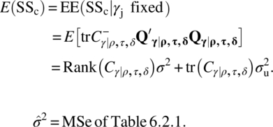
In this section, we consider the analysis of CODWR, assuming that the unit (or subject) effects are random, N = Jk,b, ui = b, and wj = k. We assume γj are distributed IIN ![]() and are independently distributed with eij. Without loss of generality, we assume
and are independently distributed with eij. Without loss of generality, we assume ![]() and
and ![]() . We now have
. We now have

From the model (6.6.1), using weighted least squares, we estimate τ and δ by τ′ and δ′, respectively, given by
and
Let w = 1/σ2 and ![]() . We combine the estimator given by Equations (6.6.2) and (6.2.3) to get the estimator of τ,
. We combine the estimator given by Equations (6.6.2) and (6.2.3) to get the estimator of τ, ![]() , given by
, given by

Similarly, combining the estimator of δ given by Equations (6.6.3) and (6.2.3), we get the estimator of δ, ![]() , given by
, given by

The dispersion matrices of these estimators are
and

To get the estimators (6.6.4)–(6.6.7), we need to estimate σ2 and ![]() . To this end, let us introduce the following notation:
. To this end, let us introduce the following notation:
![]() ,
,
The subjects’ (or units or columns) sum of squares SS0, adjusted for periods, direct and residual treatment effects, is given by
Then,

From the estimators ![]() and
and ![]() , we estimate w and w′ and complete the analysis.
, we estimate w and w′ and complete the analysis.
6.7 Concluding Remarks
In Section 6.2, the general analysis was given for CODWR when observations are taken only on treated cells (i.e., GRED-I). The analysis of GRED-II when observations are taken on treated and untreated cells can be easily developed based on the standard procedures and is left as an exercise to the interested reader. Some results on the estimability of parameter functions were also discussed in that section.
To emphasize the interest on the estimability of parametric function of τ′s and δ′s, we will give another example.
Mercado (1976) considered a 7 × 7 design for testing seven treatments by treating only 28 cells as given in the following:
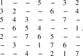
When the design was considered as GRED-I, he observed that the matrix Cδ|ρ,γ,τ has rank 7 and the matrix Cτ|ρ,γ,δ has rank 6. When the design was considered as GRED-II, both the matrices Cδ|ρ,γ,τ and Cτ|ρ,γ,δ have rank 7. The average variance of all estimated elementary contrasts of the direct and residual effects is the following:

If the experimenter decides to leave more than one cell in a BRED untreated, the pattern of untreated cells determines the estimable functions as noted in Section 6.2. An analogous situation in the case of Latin square designs was discussed by Dodge and Shah (1977).
References
- Blaisdell Jr, EA, Raghavarao D. Partially balanced change-over designs based on M – associate class PBIB designs. J R Statist Soc 1980;42B:334–338.
- Bose M, Dey A. Optimal Crossover Designs. Singapore: World Scientific; 2009.
- Bose RC, Mesner DM. On linear associative algebras corresponding to association schemes of partially balanced designs. Ann Math Statist 1959;30:21–38.
- Bose RC, Nair KR. Partially balanced incomplete block designs. Sankhya 1939;4:19–38.
- Bose RC, Shimamoto T. Classification and analysis of partially balanced incomplete block designs with two associate classes. J Am Statist Assoc 1952;47:151–184.
- Cheng CS, Wu CF. Balanced repeated measurements designs. Ann Math Statist 1980;8:1272–1283.
- Davis AW, Hall WB. Cyclic change-over designs. Biometrika 1969;56:283–293.
- Dodge Y, Shah KR. Estimation of parameters in Latin squares and Graeco-Latin squares with missing observations. Comm Statist—Theor Meth 1977;6A:1465–1471.
- Hedayat AS, Afsarinejad K. In: Srivastava JN, editors. Repeated Measurements Designs, I. A Survey of Statistical Design and Linear Models. Amsterdam: North-Holland; 1975. p 229–242.
- Hedayat AS, Afsarinejad K. Repeated measurements designs. Ann Math Statist 1978;6:619–628.
- Hedayat AS, Yang M. Universal optimality of balanced uniform crossover designs. Ann Math Statist 2003;31:978–983.
- Hedayat AS, Yang M. Universal optimality for selected crossover designs. J Am Statist Assoc 2004;99: 461–466.
- Kunert J. Optimal design and refinement of the linear model with applications to repeated measurements designs. Ann Math Statist 1983;11:247–257.
- Kunert J. Optimality of balanced uniform repeated measurements designs. Ann Math Statist 1984;11:1006–1017.
- Kushner HB. Optimal repeated measurements designs: the linear optimality equations. Ann Math Statist 1997;25:2328–2344.
- Kushner HB. Optimal and efficient repeated-measurements designs for uncorrelated observations. J Am Statist Assoc 1998;93: 1176–1187.
- Kushner HB. H-symmetric optimal repeated measurements designs. J Statist Plan Inf 1999;76:235–261.
- Laska E, Meisner M, Kushner HB. Optimal crossover designs in the presence of carryover effects. Biometrics 1983;39:1087–1091.
- Mercado R. Generalized residual effects designs [Unpublished PhD Dissertation]. Philadelphia, PA: Temple University; 1976.
- Patterson HD. The construction of balanced designs for experiments involving sequences of treatments. Biometrika 1952;39:32–48.
- Raghavarao D, Blaisdell Jr, EA. Efficiency bounds for partially balanced change-over designs based on m-associate class PBIB designs. J R Statist Soc 1985;47:132–135.
- Shah KR, Bose M, Raghavarao D. Universal optimality of Patterson’s designs. Ann Math Statist 2005;33:2854–2872.
- Stufken J. Optimal crossover designs. In: Ghosh S, Rao CR, editors. Design and Analysis of Experiments. Handbook of Statistics 13. Amsterdam: North-Holland; 1996. p. 63–90.
- Williams EJ. Experimental designs balanced for the estimation of residual effects of treatments. Aust J Sci Res 1949;2:149–168.