Math and physics are very much part of the design process!

12.1 SOME MATHEMATICAL HABITS OF THOUGHT FOR DESIGN MODELING

If a client wants a device that has reduced energy consumption as an objective (or a limit on energy consumption as a constraint), we need to have a model of our design to address our client's concerns. Similarly, if we know that users of a ladder will be unsettled by a deflection of a rung of more than 0.5 in., we need a model of the bending of the rung to figure out how to meet that as an objective (i.e., the movement should be small) or as a constraint (e.g., specifying a maximum value). When we talk about models and modeling, we use model both as a verb to denote the activity in which we think about and make representations of how devices or objects of interest behave; and as a noun to denote the representation of how devices or objects of interest behave. Those representations can be, in principle, in words, drawings or sketches, physical models, computer programs, or mathematical formulations. For our present purposes, we will focus on representing the behavior and function of real devices in mathematical terms.

12.1.1 Basic Principles of Mathematical Modeling

Mathematical modeling is an activity with underlying principles and a host of methods and tools. The overarching principles are almost philosophical in nature:

• Why do we need a model?
• For what will we use the model?
• What do we want to find with this model?
• What data are we given?
• What can we assume?
• How should we develop this model, that is, what are the appropriate physical principles we need to apply?
• What will our model predict?
• Can we verify the model's predictions (i.e., are our calculations correct?)
• Are the predictions valid (i.e., do our predictions conform to what we observe?)
• Can we improve the model?

This list of questions is not an algorithm for mathematical model building. The underlying ideas are key to problem formulation generally. Thus, the individual questions will recur often during the modeling process, and the list should be regarded as a general approach to habits of thought for mathematical modeling, which are essential for good design modeling.

12.1.2 Abstractions, Scaling, and Lumped Elements

An important decision in modeling is choosing the right level of detail for the problem, which thus dictates the level of detail for the model. We call this part of the modeling process abstraction. It requires a thoughtful approach to identifying the phenomena to be emphasized, that is, to answering the fundamental question about why a model is being developed and how we intend to use it. Stated differently, thinking about finding the right level of abstraction or detail means identifying the right scale for our model means thinking about the magnitude or size of quantities measured with respect to a standard that has the same physical dimensions.

For example, a linear elastic spring, usually expressed in terms of Hooke's law, F = kx, can be used to model more than just the relation between force and relative extension of a simple coiled spring. It can be used to describe the static load-deflection behavior of a ladder's step, and the spring constant k will reflect the stiffness of the step taken as a whole. This interpretation of k incorporates detailed properties of the step, such as the material of which it is made and its dimensions. That same spring equation can also used to model how tall buildings respond to wind loading and to earthquakes. Both of these examples suggest that we can build a simple model of a building by aggregating various details within the parameters of that model. That is, we would compile or lump together a lot of information about how the building is framed, its geometry, its materials, and so on, into a stiffness k for the ladder step or the building. We need detailed expressions for each device that allow us to aggregate their particular properties into the overarching step or building model. And, of course, we would validate our linear spring models by observing and measuring the respective behaviors of the ladder step or the tall building.

We can also use springs to model atomic bonds if we can develop or show how their spring constants depend on atomic interaction forces, atomic distances, subatomic particle dimensions, and so on. Thus, we can use a linear spring at both very small, micro scales to model atomic bonds, and at very large macro scales, as for buildings. The notion of scaling includes several ideas, including the effects of geometry on scale, the relationship of function to scale, and the role of size in determining limits—all of which we need to choose the right scale for a model in relation to the “reality” we want to capture.

Going a step further, we often say that a “real,” three-dimensional object behaves like a simple spring. When we say this, we are introducing the idea of a lumped element model in which the actual physical properties of a real object or device are aggregated or lumped into less detailed, more abstract expressions. For example, we can model an airplane in very different ways, depending on our goals. To lay out a flight plan or trajectory, we can simply consider the airplane as a point mass moving with respect to a spherical coordinate system: The total mass of the plane is lumped into a point mass; the effect of the surrounding atmosphere is modeled by introducing a retarding drag force to act on the mass point in some proportion to the mass' relative speed. To model more local effects of air moving around the plane's wings, our model would have to account for the wing's shape and surface area and be sufficiently complex to incorporate the aerodynamics of different flight regimes. To model (and design) the flaps used to control the plane's ascent and descent, our model would have to include a system to control the flaps and account for the wing's strength and vibration response. Again, what we lump into our lumped elements depends on the scale on which we choose to model, which depends in turn on our intentions for that model.

12.2 SOME MATHEMATICAL TOOLS FOR DESIGN MODELING

We now present some tools that we can use to apply the “big picture” principles to develop, use, verify, and validate mathematical models. These tools include dimensional analysis, approximations of mathematical functions, linearity, and conservation and balance laws.

12.2.1 Physical Dimensions in Design (I): Dimensions and Units

One central idea in mathematical modeling is the following: Every independent term in every equation we use has to be dimensionally homogeneous or dimensionally consistent, that is, every term has to have the same net physical dimensions. Thus, every term in a balance of mass must have the dimension of mass, and every term in a summation of forces must have the physical dimension of force. We also call dimensionally consistent equations rational equations. In fact, one important way of validating newly developed mathematical models (or of confirming formulas before using them for calculations) is to ensure that they are rational equations.

The physical quantities used to model objects or systems represent concepts, such as time, length, and mass, to which we attach numerical measurements or values. If we say a soccer field is 60 m wide, we are invoking the concept of length or distance, and our numerical measure is 60 m. The numerical measure implies a comparison with a standard or scale: Common measures provide a frame of reference for making comparisons.

We define two classes for the physical quantities we use to model problems, fundamental and derived:

• Fundamental or primary quantities can be measured on a scale that is independent of those chosen for any other fundamental quantities. In mechanical problems, for example, mass, length, and time are usually taken as the fundamental mechanical dimensions or variables.
• Derived quantities generally follow from definitions or physical laws, and they are expressed in terms of the dimensions that were chosen as fundamental. Thus, force is a derived quantity that is defined by Newton's law of motion.

If mass, length, and time are chosen as primary quantities, then the dimensions of force are (mass × length)/(time)². We use the notation of brackets [ ] to read as “the dimensions of.” If M, L, and T stand for mass, length, and time, respectively, then

Similarly, [A = area] = (L)² and [ρ = density] = M/(L)³. Also, for any given problem, we have to have enough fundamental quantities to be able to express each derived quantity in terms of those primary quantities.

The units of a quantity are the numerical aspects of a quantity's dimensions expressed in terms of a given physical standard. Thus, a unit is an arbitrary multiple or fraction of a physical standard. The most widely accepted international standard for measuring length is the meter (m), but length can also be measured in units of centimeters (1 cm = 0.01 m) or of feet (0.3049 m). The magnitude or size of the attached number obviously depends on the unit chosen, and this dependence often suggests a choice of units to facilitate calculation or communication. For example, a soccer field width can be said to be 60 m, 6000 cm, or (approximately) 197 ft.

We often want to compute particular numerical measures in different sets of units. Since the physical dimensions of a quantity are constant, there must exist numerical relationships between the different systems of units used to measure the amounts of that quantity (e.g., 1 foot (ft) = 30.48 centimeters (cm), and 1 hour (h) = 60 minutes (min) = 3600 seconds (sec or s)). This equality of units for a given dimension allows units to be changed or converted with a straightforward calculation. For example, units of pressure in the American system (psi) can be converted to units of pressure in the SI system (pascal):

Each of the multipliers in this conversion equation has an effective value of unity because of the equivalencies of the various units, that is, 1 lb ≅ 4.45 N, and so on. This, in turn, follows from the fact that the numerator and denominator of each of the above multipliers have the same physical dimensions.

We noted earlier that each independent term in a rational equation has the same net dimensions. Thus, we cannot add length to area in the same equation, or mass to time, or charge to stiffness. On the other hand, we can add quantities having the same dimensions but expressed in different units (e.g., length in meters and length in feet), although we must be very careful. The fact that equations must be rational in terms of their dimensions is central to modeling because it is one of the best—and easiest—check to make to determine whether a model makes sense, has been correctly derived, or even correctly copied!

In a familiar model from mechanics, the speed of a particle, V, due to the acceleration of gravity, g, when dropped from a height, h, is given by

Note that both sides of eq. (12.3) have the same net physical dimensions, that is, L/T on the left-hand side and [(L/T²)L]^1/2 on the right. As a result, eq. (12.3) is dimensionally homogeneous because it is totally independent of the system of units being used to measure V, g, and h. However, we often create unit-dependent versions of such equations because they are easier to remember or they make repeated calculations convenient. For example, we may be working entirely in metric units, in which case g = 9.8 m/s², so that

Equation (12.4) is valid only when the particle's height is measured in meters. If we were working with American units only, then g = 32.17 ft/sec² and

Equation (12.5) is valid only when we measure the particle's height in feet. Neither eq. (12.4) nor eq. (12.5) is dimensionally homogeneous. While these formulas may be easier to remember or use, we must keep in mind their limited validity.

There is one other way in which these dimensional considerations come into play that is worth noting. In Chapter 4, we introduced sets of units of interest for the scales of metrics to be used for assessing the achievement of objectives. These are also often called figures of merit. Similarly, to optimize a design we could construct mathematical objective functions that represent figures of merit and whose value is to be optimized. It is very important to remember that such objective functions, like equations, should likewise be rational functions: All of the independent terms in an objective function must have the same net dimensions.

12.2.2 Physical Dimensions in Design (II): Significant Figures

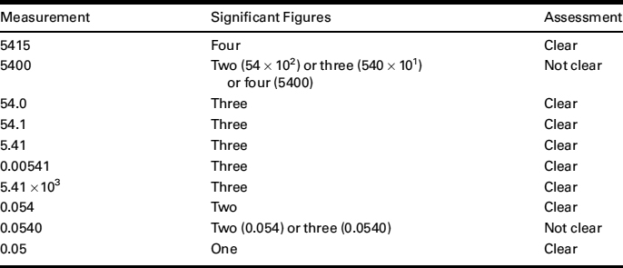
We use numbers a lot in engineering for both design and analysis, but we often need to remind ourselves about the significance of each of those numbers. In particular, people often ask how many decimal places they are expected to keep. But that's the wrong question to ask, because the number of significant figures (NSF) is not determined by the placement of the decimal point. In scientific notation, the number of significant figures is equal to the number of digits counted from the first nonzero digit on the left to either (a) the last nonzero digit on the right if there is no decimal point, or (b) the last digit (zero or nonzero) on the right when there is a decimal point. (See the examples shown in Table 12.1.) This notation or convention assumes that terminal zeroes without decimal points to the right signify only the magnitude or power of 10. In fact, confusion over the NSF arises because of the presence of terminal zeros: We don't know whether those zeroes are intended to signify something, or whether they are placeholders to fill out some arbitrary number of digits.

One way to think about the NSF is to imagine that we are running a test whose outcomes could be A, B, or C, and we want to know how often we see the result A. If A occurs four times in a set of 10 tests, then we would say that A occurs in 0.4 of the tests. If we got A 400 times in a run of 1000 tests, we would say that A was found in 0.400 of the tests—but how do we make it clear that those extra two zeroes have meaning? The answer is that we can eliminate any confusion if we write all such numbers, whether from technical calculations or experimental data, in scientific notation. In scientific notation we write numbers as products of a “new” number that is normally in the interval 1–10 and a power of 10. Thus, numbers both large and small can be written in one of two equivalent, yet unambiguous forms:

TABLE 12.1 Numbers written in different forms, together with the number of significant figures (NSF) of each and an assessment of the NSF that can be assumed or inferred. Confusion about the NSF arises because of the meaning of the terminal zeroes is not stated

Also on the subject of the NSF, we should always remember that the results of any calculation or measurement cannot be any more accurate than the least accurate starting value. We cannot generate more significant digits or numbers than the smallest number of significant digits in any of our starting data. It is far too easy to become captivated by all of the digits produced by our computers or spreadsheets, but it is really important to remember that any calculation is only as accurate as the least accurate value we started with.

12.2.3 Physical Dimensions in Design (III): Dimensional Analysis

We often find it useful to work with or even create dimensionless variables or numbers, which by design are intended to compare the value of a specific variable with a standard of obvious relevance. For example, hydrologists model some of the behavior of soil in terms of its porosity, η, which is defined as the dimensionless ratio η = V_v/V_t, where V_v is the volume of voids (or interstitial spaces) in the soil and V_t is the total volume of the soil being considered. We also see that this definition of porosity normalizes or scales the void volume V_v against the total volume V_t. A similar (and more famous) example is Einstein's formula for the relativistic mass of a particle, , in which the mass m is normalized against the rest mass, m₀, and the particle speed is scaled against the speed of light, c, in the dimensionless ratio v/c. Note that Einstein's formula is dimensionally homogeneous, and that the particle speed is normalized such that 0 ≤ v/c ≤ 1 and the mass such that 1 ≤ m/m₀ < ∞.

We can learn a lot about some behavior by doing dimensional analysis, that is, by expressing that behavior in a dimensionally correct equation among certain variables or dimensional groups. The basic method of dimensional analysis is an informal unstructured approach for determining dimensional groupings that depends on constructing a functional equation that contains all of the relevant variables, for which we know the dimensions. We then identify the proper dimensionless groups by thoughtfully eliminating dimensions. For example, consider again the free fall of a body in a vacuum described by eq. (12.3). A more general functional expression of eq. (12.3) is

The physical dimensions of the three variables in eq. (12.6) are, respectively, [V] = L/T, [g] = L/T², and [h] = L. The time dimension, T, appears only in the speed and gravitational acceleration, so that dividing V by the square root of g allows us to eliminate time and find a quantity whose remaining dimension can be expressed entirely in terms of length, that is,

If we repeat this thoughtful elimination with regard to the length dimension, we would divide eq. (12.7) by , which means that

Since we have but a single dimensionless group here, it follows that

Equation (12.9)—found with dimensional analysis alone, invoking neither Newton's law nor any other principle of mechanics—confirms eq. (12.3). This elementary application of dimensional consistency tells us something about the power of dimensional analysis. On the other hand, we do need some physics, either theory or experiment, to define the constant in eq. (12.9) that gets us to eq. (12.3).

As a further example, suppose we want to design a step on a ladder. One model of a step's behavior would be to think of its as a fixed-ended beam under a centrally applied vertical load P. We will present the appropriate model in Section 12.2.1 when we use it, but let us first see whether we can identify the form we will see by applying the basic method of dimensional analysis. We show in Table 12.2 the four derived variables for this problem and their respective dimensions: The deflection δ at the center of the beam, the load P, the beam length L, the bending stiffness EI of the beam (which is actually the product of its modulus of elasticity E and the second moment I of the beam's cross-sectional area). We also see that all of our four variables are expressed in just two physical dimensions, force (F) and length (L). We then ask, dimensionally, how does the deflection δ of the beam (or step) depend on the other four variables? That is, in analogy with our dimensional analysis of eq. (12.6), we look for the dimensionless groups embodied in the functional expression:

Since we know that the beam or step deflection has the physical dimension of length, we would eliminate the force dimension by noting that [P/EI] = L⁻² and then eliminating the force dimension by dividing accordingly:

TABLE 12.2 The four quantities chosen to model the fixed-ended beam that, in turn, will be a model for a step on a ladder. P and L are chosen as fundamental, and δ and EI are then taken as derived

Derived Quantities	Dimensions
Deflection (δ)	L
Load (P)	F
Length (L)	L
Bending stiffness (EI)	FL2

Note that eq. (12.11) also suggests that the beam's deflection varies with the ratio P/EI, which makes sense physically: increase the stiffness EI with respect to the load P and expect the deflection to decrease, and vice versa. Then, in dimensional terms, since [δ₁] = L, it follows that we need to determine a value of an exponent α such that

Clearly, α = 3 and

Equation (12.13) also confirms our physical intuition because as we make the beam or step longer, we would expect it to be more flexible, that is, to deflect more.

We can describe the basic method of dimensional analysis in a series of steps:

1. List all of the variables and parameters of a problem and their dimensions.
2. Anticipate how each variable qualitatively affects quantities of interest, that is, does an increase in a variable cause an increase or a decrease?
3. Identify one variable as depending on the remaining variables and parameters.
4. Express that dependence in a functional equation (i.e., in analogs of eqs. (12.6) and (12.10)).
5. Choose and then eliminate one of the primary dimensions to obtain a revised functional equation.
6. Repeat step (e) until a revised, dimensionless functional equation is found.
7. Review the final dimensionless functional equation to see whether the apparent behavior accords with the behavior anticipated in step (b).

12.2.4 Physical Idealizations, Mathematical Approximations, and Linearity

We generally idealize or approximate situations or objects so that we can model them and apply those models to find behaviors of interest. We make two kinds of idealizations, physical and mathematical, and the order in which we make them is important. Think of the basic pendulum: A known mass m hangs from a string of given length l. First, we identify those elements that we believe are important to the problem. We assume the string is weightless and acts only in tension, and that gravity provides the only external force. We also assume that any wind resistance is negligible and that, for now, the pendulum's swing angle θ(t) is not limited in magnitude. Our model is (still) verbal, but we have idealized several facets of the pendulum's anticipated behavior by assuming the string is weightless and by neglecting wind resistance. Soon we will also examine the consequences of considering only small angles. But for now, we have an initial physical idealization.

Second, we translate our physical idealization into a mathematical model. We have to be careful that our mathematical models are consistent with what we have assumed in our physical idealization. We start with the basic equation of motion for the pendulum, which we assume is familiar from physics. We write it here in its exact, nonlinear form, cast in terms of the pendulum's swing angle:

Equation (12.14) is a nonlinear differential equation because of the sinusoid term. Such nonlinearities make it difficult to find exact, closed-form solutions. While there is, in fact, an elegant, closed-form, implicit solution for the nonlinear pendulum, we won't discuss it as that's not our focus. Rather, we want to ask the question: Can we make a linear approximation of eq. (12.14)? If so, how, and what does that mean?

Engineers typically try to build models that are, mathematically speaking, linear models. We do this because nonlinear problems are invariably harder to solve, and also because linear models work extraordinarily well for many devices and behaviors of interest. In fact, one of the most often used linear approximations is a small angle approximation. The more common form of the small angle approximation is that of sin θ for small angles θ. In this case we have

Assuming eq. (12.15) enables us to linearize the classical pendulum problem, that is, turn it into a linear differential equation that is easily solved:

In this context, it is also worth looking at the tension in the pendulum's string,

as well as the pendulum system's potential energy,

Both eqs. (12.17) and (12.18) contain the term cos θ(t) so the equation becomes, how do we approximate that term for small angles θ(t)? This requires thinking about the meaning of “small” and in relation to what. For small angles we could have either

or

Equations (12.19a) and (12.19b) clearly present very different results, either one of which could be a suitable mathematical approximation. The “trick” is to properly understand the physical idealization that we are trying to represent, which in this case means properly identifying the scale by which we measure “small.” If we were simply approximating cos θ for small angles θ, then eq. (12.19a) would be appropriate, and, we would find from eq. (12.17) that for small angles of motion. But to approximate the potential energy of a pendulum for small angles θ, we would have to use eq. (12.19b) because in this case we're comparing (1 − cos θ) to 1, and so we would find from eq. (12.18) that for small angles of motion.

Linearity shows up in other contexts. Consider geometrically similar objects, that is, objects whose basic geometry is essentially the same. For two right circular cylinders of radius r and respective heights h₁ and h₂, the total volume in the two cylinders is

Equation (12.20) demonstrates that the volume is linearly proportional to the height of the fluid in the two cylinders. Further, we obtained the total volume using the principle of superposition (i.e., by adding the two volumes), which we could do because the volume V_cyl is a linear function of the total height h. Note, however, that the volume is not a linear function of the radius, r. That is, for different radii for the two cylinders, eq. (12.20) becomes

The relationship between volume and radius is nonlinear for the cylinders, so we can't calculate the total volume just by superposing or adding the two radii. This result is emblematic of what happens when a linearized model is replaced by its (originating) nonlinear version.

12.2.5 Conservation and Balance Laws

Many of the mathematical models used in engineering design are statements that some property of an object or system is being conserved. For example, the motion of a body moving on an ideal, frictionless path might be analyzed by stipulating that its energy is conserved, that is, energy is neither created nor destroyed. Sometimes, as in modeling the population of an animal colony or the volume of a river flow, quantities that cross a defined boundary (whether individual animals or water volumes) must be balanced. That is, we have to count or measure both what goes in to and what comes out of the boundary of the domain we're watching. Such balance or conservation principles are applied to assess the effect of maintaining levels of physical attributes. Conservation and balance equations are related: Conservation laws are special cases of balance laws.

The mathematics of balance and conservation laws is straightforward. We start by (conceptually, and sometimes graphically) drawing a boundary around the device or system we are modeling. If we denote the physical attribute or property being monitored as N(t) and the independent variable time as t, a balance law for the temporal or time rate of change of that property within the system boundary outlined can be written as

where n_in(t) and n_out(t) represent the flow rates of N(t) into (the influx) and out of (the efflux) the system boundary, g(t) is the rate at which N is generated within the boundary, and c(t) is the rate at which N is consumed within that boundary. Equation (12.18) is also called a rate equation because each term has both the meaning and dimensions of the rate of change with time of the quantity N(t).

In cases where there is no generation and no consumption within the system boundary (i.e., when g = c = 0), the balance law in eq. (12.22) becomes a conservation law:

Here, then, the rate at which N(t) accumulates within the boundary is equal to the difference between the influx, n_in(t), and the efflux, n_out(t).

Perhaps the most familiar balance and conservation laws are those associated with Newtonian mechanics. Newton's first law, usually presented as the equation of motion, can be viewed as a balance law because it refers to a balance of forces:

Note, however, that eq. (12.24) also represents a conservation law because it states the conservation of momentum: If there are no net forces acting on the mass m, then and the momentum is conserved.

The second familiar conservation principle in Newtonian mechanics is the principle of conservation of energy:

Here V represents the particular form of potential energy for the system under consideration (e.g., mgh for gravitational potential and kx²/2 for a linear spring) and E₀ is the constant total (kinetic plus potential) energy. For a nonideal system, energy is not conserved and the result is the work–energy principle:

Thus, the difference in the total (kinetic and potential) energy between states 1 and 2 is equal to the work done by the forces acting on the system as they traverse the path from state 1 to state 2.

12.2.6 Series and Parallel Connections

Almost all designs require connections, whether as simple as a mass hanging from a rope tied to a hook, or a circuit connecting a power source to a light bulb through a switch. Such connections can generally be characterized as either series or parallel. Further, we gain tremendous insights into design behavior when we link these characterizations to appropriate balance or conservation laws. We show two examples in Figure 12.1, both involving simple linear springs. The first is a series connection, where the two springs each support the same load P, while the second is a parallel connection, each deflecting the same total amount. In the series connection, we first write each spring's constitutive law, Hooke's law, as

The x_si in eq. (12.27) are absolute x-axis measurements; x_ser = x_s2 is the movement of node 2 where the load P is applied. Each spring in a series array carries the same force, F_s1 = F_s2 = P. We can then write a force balance equation at points 1 and 2 to easily calculate the total deflection of the endpoint at which P is applied:

The effective stiffness of a pair of spring in series is then

We also note that the net extension of spring 2, δ_s2 = x_ser − x_s1, can be calculated from eqs. (12.27) and (12.28) as

Equation (12.30) is interesting because it shows that a series combination of springs serves as a displacement divider because the net extension δ_s2 of spring 2 is a fraction of the total extension x_s2, and that fraction depends (here) on the ratio of the stiffness of spring 1 to the sum of the stiffnesses. Thus, if spring 1 is very stiff, it will be spring 2 that extends the most. If spring 2 is relatively stiff, then it will extend less and spring 1 will extend more. This is in accord with our intuition: Imagine a rubber rod in series with a steel rod! All of the foregoing results are readily extended to n springs in series.

Figure 12.1 Springs as one building block for mechanical systems or circuits: (a) a spring's constitutive law; (b) two springs in series; and (c) two springs in parallel.

A similar set of calculations for the common displacement and the forces in two springs connected in parallel produces similar kinds of results. The common extension of the two parallel springs is

The spring stiffnesses add linearly when they're in parallel, so that their effective stiffness is

However, and unlike its series counterpart, the forces carried by each spring in a parallel array are not the same:

We note from eq. (12.33) that a pair of springs in parallel serves as a force divider because the force in each spring is a fraction of the total force that is determined by the ratio of its stiffness to the system's effective stiffness.

The elementary electrical circuits shown in Figure 12.2 can also be viewed through the series–parallel prism. Our basic constitutive law is Ohm's law: A current I flowing through a resistor R produces a voltage drop across that resistor (see Figure 12.2(a)):

(The voltage is measured in volts (V), the current in amperes (A), and the resistance in ohms (Ω).) Figure 12.2(b) shows a voltage V₀ applied across two resistors in series. Just as two springs in series carry the same force, the two resistors in series have the same current flowing through each. The voltage drop across the two resistors in series V_ser must equal the input voltage V₀ across them, that is,

Figure 12.2 Resistors as one building block for electrical circuits or systems: (a) a resistor's constitutive law; (b) two resistors in series; and (c) two resistors in parallel.

Thus, the effective resistance of two resistors in series is simply the sum of the individual resistances:

The voltage drop across each of the resistors can be written as a fraction of the input voltage:

Thus, the two resistors in series serve as a voltage divider, reminiscent of the two springs in series acting as displacements dividers.

We can also make similar observations about the two resistors connected in parallel, as shown in Figure 12.2(c). Here we view the input as a current source, especially since the parallel nature of the circuit requires that the voltage drop across each resistor is the same as the voltage drop across that current source. This is akin to the common extension shared by two springs in parallel. What is of interest here is that the current I₀ provided by the current source divides into two components I₀ = I₁ + I₂ that share a common voltage drop V_par:

Expressed in terms of the current input, the voltage drop across this parallel circuit is

Thus, the effective resistance of this parallel circuit is

Finally, this parallel connection of two resistors acts as a current divider, as we see when we write the currents through each resistor as a fraction of the current source input:

Thus, if we compare eq. (12.41) to eq. (12.33), we see that the current divider in a parallel circuit acts very much like the force divider on the parallel mechanical circuit of two mechanical springs acting in parallel. In that vein, such dividers also exist for other linear elements in mechanical systems (e.g., dampers) and electrical circuits (e.g., capacitors and inductors).

We should not mistake the foregoing discussion as anything even remotely close to complete analyses of mechanical or electrical circuits or systems. We've shown these calculations only to point out the value of looking for series and parallel connections, whether in circuits or in very complicated systems—which can often be modeled in terms of sophisticated, lumped elements. Such series–parallel assessments provide an elegant and intuitive way to track the flow of variables through system elements (e.g., force in mechanical systems and current in electrical circuits) and changes of variables across circuit elements (e.g., displacements or movements in mechanical systems and voltage in electrical circuits). We see this clearly in the notion of dividers that apportion various inputs corresponding to element properties, a notion that is particularly interesting when sorting out functions.

12.2.7 Mechanical–Electrical Analogies

We pointed out the strong similarity between the elementary mechanical and electrical circuits we've just analyzed, which suggests there may be an analogy between the two. There is, however, also one notable difference: The mechanical elements are springs, which store energy, while the electrical elements are resistors, which actually dissipate energy (as waste heat). Does this reduce the likelihood of an analogy or diminish its utility even if there is one? In fact, there are other mechanical–electrical analogies, and they're not equally useful.

We also pointed out that the series–parallel approach applied to other elements, such as the capacitor, which has the constitutive relation

(The capacitance C is measured in Farads (F).) We see that equations in (12.42) strongly resemble their spring counterparts in (12.27), and this observation lies at the heart of the best mechanical–electrical analogy. We can liken current to force as variables that flow through elements, and voltage drops to the difference in endpoint displacements as variables that change across an element. And both capacitors and springs store energy.

Further, when we write equilibrium equations, or balance forces, we are actually conserving momentum. The corresponding electrical rule is Kirchhoff's current law, which conserves current by balancing all of the currents coming into and going out of a junction or node. Similarly, when we ensure that all of the individual spring endpoint displacements properly add up over a chain of springs, we are ensuring spatial consistency or compatibility. The electrical analogy is Kirchhoff's voltage law, which says that the sum of voltage drops around a closed circuit loop must be zero. Similarly, just as there are energy storage elements (mechanical springs, electrical capacitors and inductors), there are also energy dissipaters (mechanical dampers, electrical resistors).

A complete coverage of all of the nuances (and potential) of the mechanical–electrical analogy is well beyond our scope. However, such analogical awareness is another good habit of thought that experienced designers often exploit.

12.3 MODELING A BATTERY-POWERED PAYLOAD CART

We now illustrate how we might do some basic mathematical modeling for a fairly common design problem. In so doing, we will focus on how we formulate or set up mathematical models, rather than on solving them. Also, as we model this cart-payload-ramp design problem, we will post signs [in brackets] to indicate which modeling principles (as represented by the questions in Section 12.1.1) we are applying.

Suppose we are asked to design a cart to maximize the height h to which a payload of weight W_p can be moved up a ramp at an angle θ with the horizontal (Figure 12.3). [Why] This is a challenge on several fronts: How do we design a cart to contain and support the payload? Can we model a cart without having done its detailed design? How do we provide power to that cart, that is, how do select the appropriate battery and motor? (Note that we have implied a design solution here by assuming we're using a battery and a motor: We could perform the function of providing power with a spring.) [Assume] We'll subsume the details the cart's structural form into a parameter W_c that reflects the total weight of the cart and its battery and motor. [Assume] The basic purpose we want our model to serve is to define how much power will be needed to move the cart up the ramp. In other words, we want to identify how much electrical energy we need to transform into mechanical energy to move the cart up the ramp. [Use]

To develop a useful model, we must first decide what system(s) we want to model, and in how much detail. There are at least three ways to configure a system model [How]: The cart, battery, and motor are considered a single system within the boundary shown in Figure 12.4(a); the overall system model is decomposed into two subsystems of cart and of battery and motor, as shown in Figure 12.4(b); the overall system model is further decomposed into three subsystems of cart, battery, and motor, as shown in Figure 12.4(c). The first two models differ only if we want to distinguish between batteries that are chargeable and those that are not. Since that's a relatively unimportant difference at this stage, we will go with the two-subsystem model, wherein electrical energy is the input to the first stage, either as a new battery or as a line cord to recharge the chargeable batteries. [Given] We will formulate the overall system shown in Figure 12.4(a), and then we'll describe the virtues and the shortcomings of that model. After that, we'll provide some high-level considerations for choosing batteries and motors.

12.3.1 Modeling the Mechanics of Moving a Payload Cart up a Ramp

From the overall systems and mechanics points of view, the system inside the boundary of Figure 12.4(a) can be modeled rather simply: Consider a “particle” or lumped mass of the cart (W_c/g) and payload (W_p/g) at rest at the foot of the ramp (position 1 in Figure 12.3). Electrical energy is the input to the system (assuming an electrical cord to recharge a chargeable battery) that is transformed into mechanical energy, which is then used to move the cart up the ramp. Some of that energy will be lost due to friction, and we'll address that shortly. [Why] So our starting point is the conservation principle, expressed in the work–energy relationship of eq. (12.26) and repeated here [How]:

Figure 12.3 A sketch of the geometry and principal forces involved in modeling how a battery-powered cart moves a payload up a ramp.

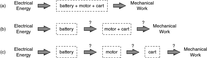
Figure 12.4 Different models of a battery energizing a motor that is in turn powering a cart require different system boundaries (shown as dashed lines): (a) a single (integrated) system; (b) a two subsystem model of (battery + motor) and the cart; and (c) a three subsystem model.

The force in the work integral in eq. (12.26) is solely dissipative because any conservative forces would be represented in appropriate potential energy terms. In the present case, both of the kinetic energy terms vanish since the cart starts and ends at rest [Assume]. Measured from a datum on the surface at the foot of the ramp, the potential energy at position 2 is

The gravitational potential energy at position 1 is zero since the cart is at the datum. However, this is the logical and convenient place to introduce the energy input, that is, the energy E_b stored in the battery. [Given] Were this a spring-loaded cart, we'd clearly write V₁ as the energy stored in an elastic spring of some (presumably given) stiffness k. Here the energy is stored in a battery:

We should note here that we must be careful when assigning a value to E_b simply because batteries and the motors they drive are not 100% efficient. While motors often are assigned efficiency ratios η (as we discuss in Section 12.3.3), it may be easier at this level of detail to reduce the value of E_b by some fraction to account for motor losses.

As we model the work done to move the cart and its payload up the ramp, we should keep in mind that friction inevitably works against us, the second law of thermodynamics being what it is [Given]. For our cart, work is done against both internal friction (e.g., in the motor's gears) and external friction (e.g., between the ramp surface and both the driver wheels as rolling resistance and the passive driven wheels as sliding friction), until the cart comes to a stop. At some point the cart will stop because we have used some of our initial energy to increase the potential energy of the cart and its payload by raising their height, and because of the aforementioned friction loss. The overall system model we're using here allows us to “disguise” the details of the different kinds friction by assuming that all of the work done against friction can be lumped together and accounted for in a simple product of the normal force of the cart (produced by the cart and payload) multiplied by a coefficient of sliding friction [Assume]:

Then, if we substitute eqs. (12.43)–(12.45) into eq. (12.26), we find the overall work–energy relationship can be put in the following form [Predict]:

Equation (12.46) is interesting and seems consistent with many of our intuitions. First, the physical dimensions of both sides of eq. (12.46) are those of work, as appropriate. Second, we see that for a given amount of battery energy, there is a clear trade-off between the total weight (W_c + W_p) and the distance d that the cart can move up the ramp. We make that trade-off more apparent by recasting eq. (12.46) to calculate the actual distance the cart moves:

We can equivalently calculate the height h to which the loaded cart is raised:

Both eqs. (12.47) and (12.48) are dimensionally homogeneous. Further, there are two limiting cases that produce results consistent with our intuitions. If the system were ideal and frictionless (i.e., ), the cart would move up the ramp up to a limiting height for which all of the battery energy has been converted into gravitational potential energy. Similarly, if there was no ramp (i.e., θ = 0), eq. (12.48) tells us that h = 0, while eq. (12.47) tells us that on a level surface, the loaded cart would travel a distance

We should keep in mind that while eqs. (12.47)–(12.49) have the virtues of dimensional consistency and reasonable limiting behavior, they also embody a lot of assumptions about the role of friction in this problem. First of all, we have no idea of what the friction coefficient really means or what its value might be. In fact, we would likely want to do both deeper analyses and some significant physical testing to see whether the basic assumptions of eq. (12.45) can be validated [Validate] or how they should be modified if not [Improve].

Further, the overall systems boundary and the simple assumption about friction mask a much more complicated problem. There are a lot of powered toy cars that we can play with—and likely have. So chances are we've seen that the driver wheels of such a toy car often spin at start-up, while the car doesn't move for some short period of time. Then the car seems to “get a grip” and take off, but often the driven wheels don't seem to turn as much as they seem to slide. This is actually a complicated mechanics problem. To start from rest, the powered driver wheels must provide enough torque to overcome static friction, which is larger than rolling resistance or sliding friction. But if too much torque is provided initially, then the wheels spin without “grabbing” the surface, which is why we see what we've just described. That means the starting torque must fall off to get the cart moving, and when the car is actually moving, we need a more complex model to describe its behavior. That in turn means that we need a more detailed mechanics model: It also means that we have to delve more deeply into how motors actually work, that is, how the torque they produce varies with the speed at which their armatures rotate. To get into the details of such modeling, we would have to work within the three subsystem boundaries defined in Figure 12.4(c) [Improve]. We won't, since that's beyond our scope, but we can't resist observing that the kind of behavior we've been describing is often seen when drivers, intentionally or not, gun their engines while starting their cars.

Before we turn to choosing batteries and motors, it is interesting to cast this design problem in the context of a design challenge or contest. Because of the weight–distance trade-offs we mentioned earlier, if we wanted to compare different cart designs, one against another, we might phrase a challenge in terms of maximizing a figure of merit (FoM) such as [Predict]:

Such a figure of merit emphasizes how the cart designers would have to trade off the distance they hope to achieve against the payload they can carry, with that payload normalized against the cart weight—which includes weights of both a battery and a motor. So there might be further refinements if, as we might expect, the available battery energy varies with battery size, and thus battery weight.

We also note that our cart design problem was stated independent of time. But suppose we wanted to get to a certain height above the datum in a specified time, which would serve as a design constraint. Or imagine that we wanted to minimize the time it would take to climb the ramp, in which case minimizing transit time would be an objective. Both of these challenges could be reflected in a revised figure of merit, namely, if we modified eq. (12.50) to read [Predict]:

In this case, we would not only need to find enough energy to move the cart, but we would also have to examine how that energy is delivered over some interval of time, that is, we need to examine its power. Thus, in searching for a battery and a motor, we need to evaluate both the time variation of a battery's energy and the operating characteristics of the motor.

12.3.2 Selecting a Battery and Battery Operating Characteristics

We start with batteries. How much energy is stored in a battery? [Why] This question is not easily answered, especially when we're buying them off a shelf. When batteries discharge their stored energy, they convert chemical energy to electrical energy as inputs to circuits. A battery can be characterized in terms of:

• voltage V (V);
• energy density E_b [typically measured in terms of either watt-hours/kilogram (W h/kg) or watt-hours/liter (W h/l)];
• capacity Q [typically expressed in ampere-hours (A h) or milliampere-hours (mA h)]; and
• the shape of the battery's discharge curve.

Depending on the particular battery, very little of this data is actually given: We most often buy batteries by their nominal voltage (e.g., 1.5 V), which is often expressed in terms of a rated physical size (e.g., AA). Battery capacity is a most important characteristic, especially when we're sizing a battery to provide a requisite power over a desired time span. In our cart-payload-ramp problem, we've not made time a particularly important variable or parameter, so we just want to know how much energy we can tap, rather than how fast or at what rate the energy is available. We can estimate that available energy from a battery's discharge curve, which we also call its operating characteristics.

We show two sets of discharge curves in Figure 12.5, along with an idealized, archetypal curve that we will use to highlight our estimates of battery capacity. Figures 12.5(a) and (b) show measured plots of voltage against time (they are readily found on the World Wide Web), and they show different curves for different current draws: The voltage drop takes longer when the current draw is lower. We also intuit that these curves reflect somehow how much energy is available. Since all of the data in these discharge curves is empirical, we need some easy estimators to get an idea of just how much energy is available, hence we use the idealized discharge curve in Figure 12.5(c) [Assume]. For that discharge curve, we identify the capacity Q as the total charge in the battery [How]. That capacity can be estimated by multiplying the draining current I_s by the time it takes to reach a precipitous drop-off in the voltage curve t_d:

The physical dimensions of Q are charge, typically measured in coulombs (C), and those of the current I_s are charge per unit time, with normal units of amperes (A = C/s). However, because of the ranges of the numbers involved, battery capacity is typically expressed in units of ampere-hours (A h = A s/3600) or milliampere-hours (mA h). So, depending on both the resistance through which the battery drains and its discharge current, Figure 12.5(a) suggests (roughly) that Q_AA = (1.4)(1) = 1.4, (3.6)(0.5) = 1.8 or (8.2) (0.25) = 2.05 A h [Find]. The capacity of the LR44 is noticeably lower, as can be estimated from Figure 12.5(b): Q_LR44 = (675)(181.8 × 10⁻⁶) = 0.122 A h [Find]. An LR44 battery has less capacity than an AA, draws much less current, and is physically much smaller than a AA. That is why LR44s are used in devices where they are exchanged infrequently, for example, watches and calculators.

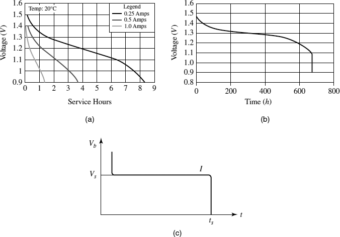
Figure 12.5 Battery discharge curves or battery operating characteristics: (a) AAs for different currents; (b) LR44 at 181.8 μA; and (c) an idealized, archetypal discharge curve with nominal service voltage V_s, service time t_s, and draining current I_d.

The energy stored in a battery can then be estimated as [Predict]:

In eq. (12.53) we have introduced the average service voltage V_s, which we usually estimate by looking for the plateau in a battery's discharge curve. Further, it is quite clear from the idealized battery discharge curve (Figure 12.5(c)) that eq. (12.53) is an estimate of the area under the discharge curve. E_b has the physical dimensions of voltage × current × time or voltage × charge, which are the appropriate dimensions for electrical work. For the case of the LR44 battery, whose operating capacity is shown in Figure 12.5(b), that plateau is fairly evident, , and so [Find].

We should use the calculated value of E_b with some caution, principally because we are not accounting for any losses in the battery itself or in the ways we connect it to whatever device we use to do the mechanical work we want done [Why]. The simplest way to model this aspect is to recognize that a battery is an emf: A device that converts chemical, mechanical or some other from of energy into electrical energy. It has a (voltage) value V_b. The emf is connected in series to the battery's own internal resistance R_b and to another resistor R that represents a load (see Figure 12.6) [How]. That resistor could represent a simple way to dissipate energy through a resistance load, or it could be a simple stand-in for a motor with the power, otherwise dissipated, being fed into some transmission device to do mechanical work [Assume]. In our case, we would regard that power “loss” as providing the energy needed to do the work of moving the loaded cart up the ramp.

Figure 12.6 Circuit of a battery with emf V_b and internal resistance R_b connected to a load resistor R, which can also serve as an elementary model for the load imposed by a motor.

The circuit in Figure 12.6 is relatively simple. It has a single loop current I, and we can analyze it by balancing the voltage drop across the two points a and b, which yields the following instance of Kirchhoff's voltage law [Predict]:

Since R_b represents the battery's internal voltage, we may regard the term (V_b − IR_b) as the net voltage available at the battery's terminals (think car batteries!). The power output across the resistance R is [Predict]

We obtain the second form of eq. (12.55) by eliminating the current I, which we found from the Kirchhoff statement (12.54). The physical dimensions of power are those of work/time, and the corresponding metric units are watts or joules/seconds (W = J/s).

Remembering that we regard this as useful power output in our elementary model of a motor as the resistor, we would like to develop the motor's maximum power. Thus, using classical calculus, we evaluate

We find the maximum power is developed when the motor's resistance equals that of the battery (i.e., R = R_b), and that maximum power is

There will inevitably be losses in a real motor, and in any attached transmission components (e.g., gears). So, it would be extraordinarily optimistic to simply accept the calculated values of E_b (eq. (12.53)) and P_max (eq. (12.57)) without considering how both the battery and the motor are actually situated and used in the overall cart design.

12.3.3 Selecting a Motor and Motor Operating Characteristics

We finished our description of battery behavior by modeling a motor as a resistor in series with a battery. That's all well and good as far as it goes, but it is also useful to think a little about how a simple motor operates, particularly in terms of its output. A motor can be characterized in terms of:

• angular speed ω [typically measured in units of revolutions per minute (rpm)];
• torque T [with physical dimensions of F·L and measured in the metric system in units of (N m) and in the British system in (lb_f ft)];
• gear ratio n [dimensionless ratio of the number of teeth on the driving gear to the number of teeth on the driven (output) gear];
• power P [with physical dimensions of F·L/T and measured in the metric system in units of (W or N m/s) and in the British system in (hp or lb_fft/sec)];
• motor efficiency η [dimensionless ratio P_out/P_in]; and
• the shape of the motor's characteristic operating curve.

As we noted just above, a major descriptor of a motor is the shape of its characteristic operating curve, which is a plot of the motor torque against its rotational speed. For DC motors generally, the relationship of torque to rotational speed is given by:

Equation (12.58) is plotted in Figure 12.7, with the aid of which we can see why T_s is called the stall torque: it is the torque at which the motor stalls or stops turning (i.e., ω = 0); and ω₀ is called the no-load speed because it is the speed at which there is no load on the motor (i.e., T = 0). Further, the power produced by such a DC motor can be calculated as:

From eq. (12.59) we can easily show that the motor produces a maximum power at one-half of the no-load speed with the corresponding torque being one-half of the stall torque, that is,

Figure 12.7 The torque vs. speed operating characteristic curve for a DC motor.

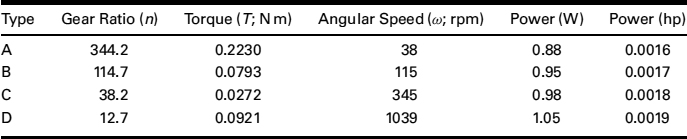
TABLE 12.3 Operator characteristics of typical geared DC motors, arranged in order of their decreasing gear ratios

Practically speaking, experts employ some rules of thumb aimed at maximizing motor efficiency when they are choosing motors to provide a specific torque and a specific operating speed. Those heuristics are that the motor:

• should run at 70–90% of the no-load speed (ω₀); and
• should provide a torque of 10–30% of the stall torque (T_s).

Generally, when we choose a motor to provide a specific torque while running at a specific speed, we also need to account for the gearing that comes along with the motor because the gear ratio is a property of that motor. In Table 12.3 we show data for a small, geared DC motor, drawn from a manufacturer's catalogue. We've extended the manufacturer's data to show two sets of torque values. The first set shows T values in nonstandard units of gf cm, a practice that is not uncommon in many such catalogues. Why would someone use such nonstandard units? Perhaps the answer follows from the second set of T data, expressed in the more customary N m, and for which the numbers are small: When doing quick hand calculations, which we often do in this kind of modeling, it's easier to deal with the numbers that arise when T is measured in those nonstandard units. Note, too, that the data as given (and extended) do not explicitly identify the power outputs of the four motors listed.

The power produced by a motor is simply the product of the torque and the angular speed. In standard metric units the power is

In conventional American units the power is

We have calculated the power output of each of these motors and show the data in Table 12.4. Clearly, the four motors listed all produce almost the same (small) amount of power, at an average of P_out/ave = 0.96 W = 0.0018 hp. However, we can see by reading up the table (from the bottom row) that the power drops off as the gear ratio increases. This is common and perhaps ought to be another motor heuristic: an increase in the gear ratio will produce a decrease in the power delivered. Thus, while we can provide more torque by using a higher gear ratio, it comes at the cost of both a lower speed and less power (i.e., fewer watts or lower horsepower numbers). These results seem intuitively right.

TABLE 12.4 Power outputs of typical DC motors, arranged in order of their decreasing gear ratios

It also turns out that many of the small motors characterized as those in Table 12.3 are designed to work with batteries of a particular voltage. Thus, all of the motors in Table 12.3 run on 3 V batteries. So the battery–motor combination is fixed, once we choose such a motor.

Finally, although this would not likely come into play for the kinds of small toy motorized carts we have been talking about, it turns out that one major issue in motor selection is that they generate a fair amount of heat. The amount of heat generated will be a consequence of the current I through the motor's resistance R, as specified by eq. (12.55). Again, for small-scale models and toys, this should not be an issue since we are talking about very small amounts of power.

We now know the principles of sizing a battery and choosing a motor, so we can design a cart—at least to the extent of balancing the payload-to-cart weight ratio against the distance d moved up the ramp, as a function of the chosen E_b, and as a function of P_out if time is important in our design. We may also view the battery as a constraint, for example, when only certain batteries are available, or perhaps because of cost considerations. And, of course, we have to remember that the physical size of the battery and the motor will also enter into our design considerations because its weight is part of the overall cart weight.

12.4 DESIGN MODELING OF A LADDER RUNG

We now model and design the step or rung of a ladder to show how modeling is needed to do design properly. In order to design a ladder's step we need a model that predicts its behavior [Why], which means that we want to be able to understand how the step's attributes (e.g., size, shape, material, connections to the ladder's frame) affect its ability to support given loads [Find]. We are told that the ladder must support a person of specified weight W_p carrying a specified weight W_w [Given]. We will model the behavior of the step (and the ladder) using a standard model of linear elastic beam behavior (described in Section 12.4.1) and standard models of the elastic behavior of materials [Assume]. We will develop and apply the model of the step using basic principles of mechanics [How] and show just how the total weight that it can support depends on its geometric and material properties [Predict]. Note how we are limiting our modeling effort: At this point we are not analyzing the size, shape, or materials of the side frames, any cross bracing, or any footpads on a rung. We are also precluding any linkages among the various ladder supports. One or more mathematical models would be needed to develop these parts of the ladder, but we will just model an individual rung or step.

Figure 12.8 Free-body diagrams (FBDs) of various aspects of a person standing on a ladder: (a) side-elevation FBDs of person and ladder taken as a system; (b) a front-elevation FBD of the ladder showing vectors of the force F_normal = P = W_p + W_w due to the person standing on a rung, as well as the vertical forces (R_L, R_R) and moments (M_L, M_R) by which the ladder's side rails support the rung. Courtesy of S. D. Sheppard and B. H. Tongue. Reprinted by permission of John Wiley & Sons, Inc.

Let us now apply some basic mechanics principles. In Figure 12.8 we show three sketches of a person on a ladder, the first of which is a free-body diagram (FBD) of the person and the ladder taken as a system. The second sketch shows an FBD of the entire ladder. The third drawing shows elevations of FBDs of the rung, on which are shown vectors representing (a) the force exerted by the load-carrying person and (b) the vertical forces and moments provided by the ladder's frame to support the step.

12.4.1 Modeling a Ladder Rung as an Elementary Beam

Imagine the two scenarios shown in Figure 12.9, both of which show a vertical load P supported by a transverse (i.e., normal or, here, horizontal) element. Figure 12.9(a) shows a cable or rope, along with FBDs of two sections of the cable. We see that the load seems to make the cable kink, and that a vertical load can be supported by a tensile force T in the cable or rope. In Figure 12.9(b) we show a beam, along with two FBDs of the beam divided into two sections. In the first FBD, we see that the external vertical force in each section is supported by reactions R_A and R_B at each beam support and an internally developed shear force, V. However, there is nothing to prevent either section from rotating or spinning because each has an unbalanced couple or moment in the configuration shown. In the second beam FBD we have included bending moments M that are internally developed couples (or moments) that maintain moment equilibrium and thus prevent each section from spinning out of control. These bending moments are developed by in-plane stresses along the axis of the beam, so that it is a set of horizontal stresses that support a vertical load in a beam!

For our purposes, the important aspects of elementary beam theory are that beams behave like linear springs and the stiffness of a beam depends on several of the beam's parameters. For a simple beam, a load P applied at the mid-way point of a beam of length L produces a deflection δ of the beam under that point:

Figure 12.9 Supporting a vertical force with a transverse (horizontal) structure: (a) cable and FBDs of two sections of the cable; and (b) a beam and a FBD of one section of the beam that also shows how a moment (couple) is developed by axially directed normal stresses on the beam's cross-sectional area.

Here C_δ is a number that changes with the beam's boundary conditions. (We used dimensional analysis to derive this result as eq. (12.13), and showed the dimensions of the variables involved in Table 12.2.) We can also rewrite eq. (12.63a) as an analog of the classical spring formula, F = kx, that is,

The other physical quantity of great interest in beam theory is the bending stress along the axis of the beam. As may be visualized from Figure 12.9(b), it is the bending stress that creates the bending moment and its consequent shear force that enables a long thin beam to support a load that acts in a direction normal to the (long) axis of that beam. The maximum stress in a loaded beam is

Here h is the height of the beam's cross-section (see, again, Figure 12.9) and C_σ is a number that changes with the beam's boundary conditions. Stress has the same physical dimensions as pressure, that is, [σ] = F/L².

The classical spring formula has only one constant or design variable that can be chosen or manipulated, k, which thus limits its design freedom. For the beam that has to span a given length L, there are three variables that can be varied: E, I, and h. (To the extent we can choose how the beam is supported at its ends, we can also choose between appropriate pairs of constants, C_δ and C_σ). The increased number of variables means that we can design to achieve objectives or constraints expressed in terms of the beam's deflection (eq. (12.63a)) and its maximum stress (eq. (12.64)). Thus, we shall soon talk about designing the beam for stiffness, when the deflection is our focus, or designing the beam for strength, when the maximum stress is our focus.

We see in Figure 12.10 that there are different rung supports (or connections) to stipulate or model. The two limiting cases that are of most relevance are pictured in Figure 12.11: Simple (or pinned or hinged) supports that provide a vertical reaction force and prevent any vertical deflection but leave the ends of the beam free to rotate; and fixed (or rigid or clamped) supports that provide both vertical reaction forces that prevent vertical deflections and moments that force the slope of the deflection of the beam to vanish (i.e., the moments prevent any rotation at that support). These two limiting cases, informed by our actual experience, suggest that we will have to make another modeling-design assumption when we design the rung.

With eqs. (12.63) and (12.64) in hand, and a tentative decision taken about the kinds of beam supports we will consider, we have specified the equations we will use, the calculations we can make and the types of answers we might expect [Predict]. Thus, we have established a principled model that we can now use for the preliminary design of a ladder rung.

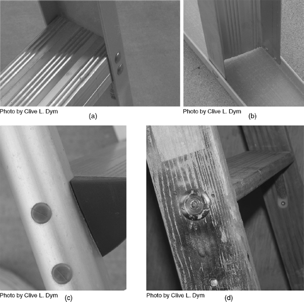
Figure 12.10 Connecting ladder rungs to ladder frames. (a, b) Top and bottom views of how metal rungs are attached to a ladder's fiberglass frame; note the gap between the top surface of the rung and the frame, so the support is neither simple nor fixed. (c) On this metal ladder the connections go through the frame into the hollow (curved) box that forms the rung; it is also an intermediate support. (d) This very old wooden stepladder has solid rungs that are bolted to the frame, but there are extra (partially visible) supports that bring the connection closer to fixed or clamped.

12.4.2 Design criteria

What are our design criteria, that is, against what requirements do we assess the performance of our designs? In part, that depends on both our objectives and our constraints. We identified some top-level objectives during conceptual design:

• light weight, that is, minimize the mass of material used in the ladder; and
• inexpensive, that is, minimize the cost.

Figure 12.11 Some aspects of elementary beam models: (a) rectangular, hollow box, I-beam and channel cross-sections, including thicknesses (h) and second moments (l); (b) a beam with simple supports at both ends; and (c) a beam with fixed supports at both ends.

We should keep in mind that the relative importance of these two objectives will vary with our client and application: Mass is far more important for a ladder to be used on a space vehicle, while a “big box” retailer is more likely to worry about cost. But there are two other design aspects that must be considered and that can be categorized either as objectives or as constraints. Those two issues derive from not wanting the rung to break or fail when someone stands on it, and not wanting the rung to deflect too much lest that someone feel uncomfortable. We need to specify what it means to require that the rung “not break or fail” and “not deflect too much.” And we need to specify whether these are both (possibly competing) objectives, constraints, or some combination.

A material breaks or fails when any one of three failure strengths is exceeded. When we determine values of the design variables such that the rung's bending stress does not exceed specified failure strengths, we are designing for strength. The three failure strengths are values of the stresses at which a material fails under, respectively, a tensile stress, a bending test, or a tensile test that produces permanent deformation. These three failure strengths are materials properties that have been measured and tabulated for most materials. As a result, this aspect of our design problem is in part a materials selection problem. We can generally lump the three modes of failure together and refer to the minimum of the three for a given material as the failure strength of interest, σ_f. Since material properties are largely established through laboratory testing and experience, our degree of confidence varies with the material. We reflect that variation of confidence by stating that the failure strength should be divided by a safety factor S, with S being as low as 1.2 for well-understood materials and as high as 5 for materials for which the properties are not as well established. (Of course, other uncertainties can be incorporated into S.) Then the strength requirement would be expressed in terms of the bending stress as σ ≤ σ_f/S. Failure strengths typically have values on the order of a megapascal, 1 MPa = 10⁶ Pa, where the pascal (Pa) is the SI unit of stress defined as 1 Pa = 1 N/m².

A rung deflects too much when a specified maximum deflection is exceeded. When we determine values of the design variables such that the rung's midpoint deflection does not exceed specified deflection limits, we are designing for stiffness. The specified upper limit generally follows from ergonomic considerations: We don't want a ladder to feel wobbly when we are standing on a rung. Thus, codes or standards often specify a maximum deflection δ_max as a fraction of the rung's length, L. The deflection requirement would then be expressed in terms of the deflection as δ ≤ δ_max ≤ C_dL, where C_f is a very small number, say C_d ~ L/100.

We now address one last loose (design) end: Do we choose pairs of constants, C_δ and C_σ, to correspond to beams with simple supports or to beams with fixed supports? Experience suggests that the ends of a step would be most accurately modeled as fixed or clamped. However, since the side rails of the frame are not truly rigid, there will always be a (very) small amount of rotation at the rung's ends (see Figure 12.10). Thus, we will model the rung as a beam on simple supports, knowing it will be a more flexible (and thus more conservative) model that will overpredict both the stress in and the deflection of the step [Assume]. As a result, our final design will bend less and carry bigger loads than our model predicts. The values of the constants for simple supports, C_δ = 48 and C_σ = 4, are found from exact solutions for the deflection and the bending stress of a simple beam carrying a vertical load P at its midpoint.

To summarize, we have four objectives to achieve: We want to minimize both the mass and the cost, subject to both the strength constraint and the stiffness (or deflection) constraint. There are several ways to proceed. We could simply look at how the mass and the cost vary with different materials and then assess designs for both strength and stiffness. If we were experienced structural designers or our intuition were sufficiently well developed, we might note that the stiffness constraint is usually much more severe than the strength constraint. That is, if the stiffness constraint (δ ≤ δ_max = C_fL) is met, it is rather unlikely that the strength constraint (σ ≤ σ_f/S) will be violated. If such a case emerged, we might have to revise our objectives for cost and our constraint on stiffness, and then check again whether the strength is sufficient. We also want to ensure that we get a reasonable result for the step thickness. For example, polymer foams may be superior in both cost and stiffness, but the final step thickness may be 0.5 m, which is clearly impractical for a ladder. (Such a large thickness would also violate the assumptions underlying the beam model whose results are given in eqs. (12.63) and (12.64). [Validate])

12.5 PRELIMINARY DESIGN OF A LADDER RUNG

We now undertake some elements of preliminary design. In the “real” preliminary design of a ladder we would consider beams of various cross-sections and likely make some estimates of which shapes are likely to be more efficient when made of different materials. We might then choose one shape for further development, along with a range or set of materials. Then, in “real” detailed design we would refine that design by working to optimize it, making it as light and cheap as possible. We would also decide how to attach the rungs to the ladder frame (e.g., with rivets, welds, or bolts) and then “size” and fix the locations of those attachments. In our case, we will use preliminary design to illustrate and contrast materials selection when designing for strength and when designing for deflection (or stiffness). In our detailed design we will optimize rung designs to achieve minimum mass and minimum cost.

12.5.1 Preliminary Design Considerations for a Ladder Rung

With both failure and deflection criteria defined, and both loose ends tied up, our design problem is that we want the rung's midpoint deflection δ and its maximum bending stress σ to satisfy

and

and where P represents the combined weight of someone standing on the ladder and of the package that person is carrying, that is, P = W_p + W_w. An important question is, do we treat these as inequalities (objectives) or do we adopt the equal signs (constraints) for both the deflection and the stress? The answer is that we cannot treat both as constraints. While there are nominally three design variables (E, I, h), I and h are so strongly related that they are effectively a single variable. Still more important, E and I (and h) are not truly independent variables. In fact, as we pointed out in the discussion that follows eq. (12.64), the material property (E) and the geometric properties (I or h and L) are incorporated into a single effective stiffness, namely, k_eff = 48EI/L³. The implication of this is that we can design for strength or we can design for stiffness, but we cannot design for both at once. Thus, we can choose to minimize the deflection, in which case we are designing for stiffness and we must then check to ensure that the corresponding bending stress is below the failure criterion. To design for stiffness, we start by equating the bending stress to the failure strength, after which we calculate the corresponding deflection and assess whether we can (or not) accept that value.

As noted, the rung's effective stiffness depends on both material and geometric properties. In many structural design problems, the material is chosen or specified in advance. In that case, the design variable that remains is the cross-sectional area of the rung as represented by its second moment, I. As shown in Figure 12.11(a), the second moment I and the rung's thickness h can be used to model a wide variety of shapes, including rectangular cross-sections, I-beams, and channel sections. The reasons that I-beams, channels, and similar such sections are widely used are that they are more efficient than rectangular cross-sections in that they sustain higher stresses per unit weight, and that modern material processing capabilities make it easy to manufacture such shapes in great volume. In fact, if we look again at Figure 12.10, we see that only the wooden ladder rung has a complete rectangular cross-section. However, knowing that our results will perhaps be unrealistic, we will limit our exploration of this aspect of the design space by assuming that the step has a rectangular cross-section, with width b [Assume]. In this case, then, I = bh³/12, and our current set of design variables has changed from E, I, and h to E, b, and h.

Finally, we will also assume that the rung width b is constrained, as in fact it is. For example, the American National Standard for Ladders—Wood Safety Requirements (published by The American National Standards Institute) stipulates fixed rung widths for a variety of wooden stepladders. Thus, even though we are not constraining our design to wooden rungs, we will assume that the width b is a specified quantity [Assume]. As a result, we now actually have only two design variables, E and h.

12.5.2 Preliminary Design of a Ladder Rung for Stiffness

We now formulate the first of two different preliminary design problems for rungs of rectangular cross-sections and fixed widths, namely, we design for stiffness by constraining the deflection. We do that because we don't know in advance what stiffness is required to achieve a specified deflection, although we do know (and specify) the limiting value that we place on that deflection. We might also think of design for stiffness as design for deflection. In eq. (12.65) we see that C_δ = PL²/48EI, which then yields

Equation (12.67) can be solved for the thickness design variable, h:

Equation (12.68) determines the rung thickness and its value clearly depends on the given values of P, L, b, and C_f, as well as on the value of the modulus E, which is as yet unspecified. Typically we would have a range of materials in mind (e.g., aluminum, steel, wood, or a composite for a ladder), and we would calculate the corresponding thicknesses of our rung accordingly. However, we have to ensure that the step does not fail, and thus by substituting eq. (12.68) into eq. (12.67) we would check that

TABLE 12.5 Possible designs of the rung of a ladder for stiffness. The design load (i.e., the weight supported) is P = 1350 N; the rung length L = 350 mm; the rung width b = 75 mm; the safety factor is S = 1.5; and the constraint constant C_d = 0.01. Note that two of the materials, aluminum and wood, violate our strength constraint that σ/(σ_f/S) ≤ 1

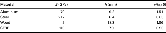
Or, with the stress cast in a dimensionless ratio,

In Table 12.5 we show some thickness and modulus values of possible rungs designed to meet the stiffness constraint. We note that the thicknesses all seem reasonably small, but that the ratio of the stress to the failure stress, σ/(σ_f/S), is not always less than 1. Our intuition that the stiffness constraint would be more severe than the strength constraint turned out to be false for two of the materials, although the wood rung is a very near miss, even with a small safety factor. [Verify] A different kind of wood might have produced a more satisfying result. However, these results confirm one of the basic reasons for making a model, that is, to (numerically) check on our intuition.

12.5.3 Preliminary Design of a Ladder Rung for Strength

We design for strength by constraining the stress to ensure that failure does not occur. We then have to calculate the corresponding deflection and decide whether we can accept that deflection. Thus, the statement of designing for strength begins with eq. (12.68), σ = PL/8hI = σ_f/S, which means constraining the stress such that

We now solve for the thickness design variable, h, using the constraint (12.71):

Then the deflection that corresponds to this strength design is formulated by substituting eq. (12.72) into eq. (12.65):

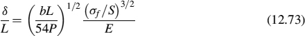
Note, too, that here we have cast the deflection in a dimensionless ratio.

TABLE 12.6 Possible designs of the rung of a ladder for strength. The design load (i.e., the weight supported) is P = 1350 N; the safety factor is S = 1.5; the rung length is L = 350 mm; and the rung width b = 75 m. Note that two of the materials, steel and CFRP, violate our stiffness constraint that δ/L ≤ 0.01

In Table 12.6 we show some results for strength design for the same four materials listed in Table 12.5. Here, too, the thicknesses all seem reasonably small, but the ratio of the midpoint deflection to the rung length, δ/L, is sometimes—but not always—larger than the 0.01 limit prescribed in the stiffness design. The two materials that failed the strength constraint in the stiffness design, aluminum and wood, here pass the stiffness constraint in the strength design, and vice versa for the other two, steel and CFRP. We were right only half of the time with our assumption about stiffness being a more severe constraint than strength. [Verify]

12.6 CLOSING REMARKS ON MATHEMATICS, PHYSICS, AND DESIGN

We have seen that preliminary design requires both careful mathematical modeling and appropriately focused research to obtain relevant data. We have examined two cases of mathematical modeling and their results, but designing beams and doing research to identify appropriate materials are both eminently practical skills in their own right. Further, the lessons regarding dimensions, scaling, simplifying assumptions, and how a model answers only the questions asked of it are lessons that can be applied to almost all modeling (and design) efforts.

One of the reasons that engineering programs emphasize engineering science content is a reflection of the extent to which such modeling and related research activities must be performed to do good engineering.

12.7 NOTES

Section 12.1: The discussion of mathematical modeling has its roots in Dym (2004) and Dym (2007).

Section 12.2: The modeling of beams is taken from Dym (1997), while the approach to material selection is due to Ashby (1999).

Section 12.3: Again, the approach to material selection, especially the use of materials selection charts, is based on Ashby (1999).