5. Performing Calculations Within Pivot Tables
Introducing Calculated Fields and Calculated Items
When analyzing data with pivot tables, you often need to expand your analysis to include data based on calculations that are not in your original data set. Excel provides a way to perform calculations within your pivot table through calculated fields and calculated items.
A calculated field is a data field you create by executing a calculation against existing fields in the pivot table. Think of a calculated field as adding a virtual column to your data set. This column takes up no space in your source data, contains the data you define with a formula, and interacts with your pivot data as a field—just like all the other fields in your pivot table.
A calculated item is a data item you create by executing a calculation against existing items within a data field. Think of a calculated item as adding a virtual row of data to your data set. This virtual row takes up no space in your source data and contains summarized values based on calculations performed on other rows in the same field. Calculated items interact with your pivot data as a data item—just like all the other items in your pivot table.
With calculated fields and calculated items, you can insert a formula into your pivot table to create your own custom field or data item. Your newly created data becomes a part of your pivot table, interacts with other pivot data, recalculates when you refresh, and supplies a calculated metric that does not exist in your source data.
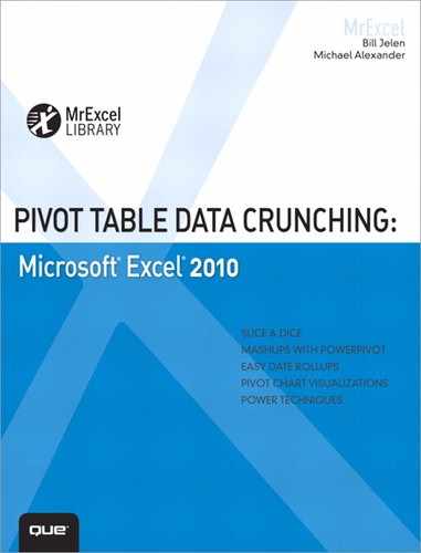
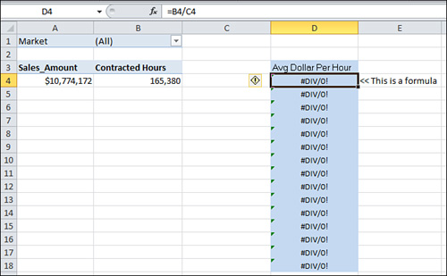
The example in Figure 5.1 demonstrates how a basic calculated field can add another perspective on your data. Your pivot table shows total Sales_Amount and Contracted Hours for each market. A calculated field that shows you Avg Dollar Per Hour enhances this analysis and adds another dimension to your data.
Figure 5.1 Avg Dollar Per Hour is a calculated field that adds another perspective to your data analysis.
Now, when you look at Figure 5.1, you might ask, “Why go through all the trouble of creating calculated fields or calculated items? Why not just use formulas in surrounding cells or even add your calculation directly into the source table to get the information you need?”
To answer these questions, the following sections discuss the three different methods you can use to create the calculated field shown in Figure 5.1.
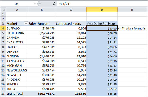
Method 1: Manually Add the Calculated Field to the Data Source
You can manually add a calculated field to your data source, as shown in Figure 5.2, which allows the pivot table to pick up the field as a regular data field.
Figure 5.2 Precalculating calculated fields in your data source is both cumbersome and impractical.
On the surface, this option looks straightforward. However, this method of precalculating metrics and incorporating them into your data source is impractical on several levels.
For example, if the definitions of your calculated fields change, you have to go back to the data source, recalculate the metric for each row, and then refresh your pivot table. If you add a metric, you have go back to the data source, add a new calculated field, and then change the range of your pivot table to capture the new field.
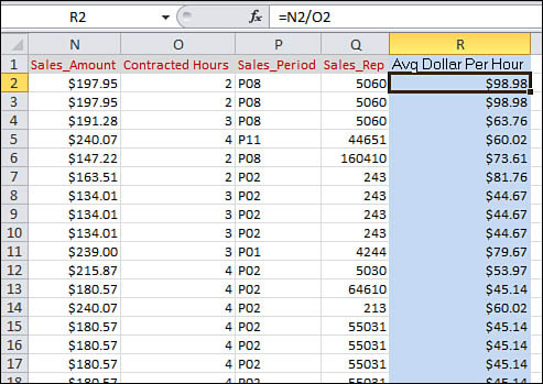
Method 2: Use a Formula Outside the Pivot Table to Create the Calculated Field
You can add a calculated field by performing the calculation in an external cell with a formula. In the example shown in Figure 5.3, the Avg Dollar Per Hour column is created with formulas referencing the pivot table.
Figure 5.3 Typing a formula next to your pivot table essentially gives you a calculated field that refreshes when your pivot table is refreshed.
Although this method gives you a calculated field that updates when your pivot table is refreshed, any changes in the structure of your pivot table have the potential of rendering your formula useless.
As you can see in Figure 5.4, moving the Market field to the report filter area changes the structure of your pivot table, which exposes the weakness of makeshift calculated fields that use external formulas.
Figure 5.4 External formulas run the risk of errors when the pivot table structure is changed.
Method 3: Insert a Calculated Field Directly into the Pivot Table
Inserting the calculated field directly into your pivot table is the best option because this method provides the following advantages:
• Eliminates the need to manage formulas
• Provides for scalability when your data source grows or changes
• Allows for flexibility in the event that your metric definitions change
• Alters a pivot table’s structure
• Measures different data fields against a calculated field without worrying about errors in formulas or losing cell references
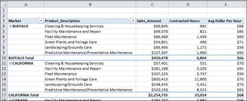
The pivot table report shown in Figure 5.5 is the same one you see in Figure 5.1, except it has been restructured so you get the Avg Dollar Per Hour by market and product.
Figure 5.5 Your calculated field remains viable even when your pivot table’s structure changes to accommodate new dimensions.
The bottom line is that there are significant benefits to integrating your custom calculations into your pivot table, which include the following:
• The elimination of potential formula and cell reference errors
• The capability to add and remove data from your pivot table without affecting your calculations
• The capability to auto-recalculate when your pivot table is changed or refreshed
• The flexibility to change calculations easily when your metric definitions change
• The capability to manage and maintain your calculations effectively
Creating Your First Calculated Field
Before you create a calculated field, you must first have a pivot table. Therefore, begin by building the pivot table shown in Figure 5.6.
Figure 5.6 Create the pivot table shown here.

Now that you have a pivot table, it is time to create your first calculated field. To do this, you must activate the Insert Calculated Field dialog box. Select Options under the PivotTable Tools tab, and then select Fields, Items & Sets from the Tools group. Selecting this option activates a drop-down menu from which you can select Calculated Field, as shown in Figure 5.7.
Figure 5.7 Start the creation of your calculated field by selecting Calculated Field.

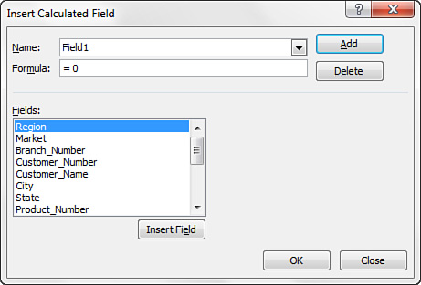
Excel activates the Insert Calculated Field dialog box, as shown in Figure 5.8.
Figure 5.8 The Insert Calculated Field dialog box assists you in creating a calculated field in your pivot table.
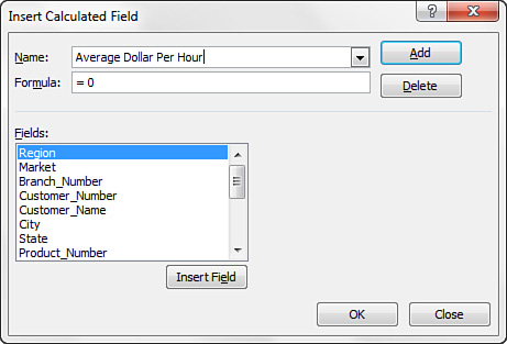
Notice the two input boxes, Name and Formula, at the top of the dialog box. Give your calculated field a name, and then build the formula by selecting the combination of data fields and mathematical operators that provide the metric for which you are looking.
As shown in Figure 5.9, first give your calculated field a descriptive name. For example, you might choose a name that describes the utility of the mathematical operation. In this example, enter Average Dollar Per Hour in the Name input box.
Figure 5.9 Give the calculated field a descriptive name.
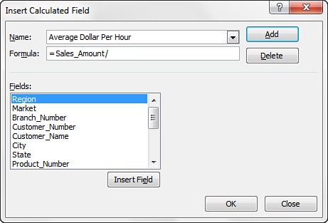
Next, go to the Fields list and double-click the Sales_Amount field. Enter / to let Excel know you plan to divide the Sales_Amount field by something.
Caution
By default, the Formula input box in the Insert Calculated Field dialog box contains = 0. Be sure to delete the 0 before continuing with your formula.
At this point, your dialog box should look similar to the one shown in Figure 5.10.
Figure 5.10 Start your formula with = Sales_Amount.
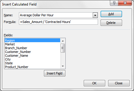
Next, double-click the Contracted Hours field to finish your formula, as shown in Figure 5.11.
Figure 5.11 The full formula, = Sales_Amount/’Contracted Hours’, gives you the calculated field you need.
Finally, select Add and then click OK to create your newly created calculated field.
As you can see in Figure 5.12, not only does your pivot table create a new field called Sum of Average Dollar Per Hour, but the PivotTable Field List includes your new calculated field as well.
Figure 5.12 Although your calculated fields don’t go to your source data, they will show in your PivotTable Field List.

Note
The resulting values from a calculated field are not formatted. However, you can apply any desired formatting using some of the techniques you learned in Chapter 3, “Customizing a Pivot Table.”
Does this mean you have just added a column to your data source? The answer is no. Calculated fields are similar to the pivot table’s default subtotal and grand total calculations in that they are all mathematical functions that recalculate when the pivot table changes or is refreshed. Calculated fields merely mimic the hard fields in your data source, enabling you to drag them, change field settings, and use them with other calculated fields.
Take a moment to look at Figure 5.11 closely. Notice that the formula you entered uses a format similar to the one used in the standard Excel formula bar. The obvious difference is that instead of using hard numbers or cell references, you are referencing pivot data fields to define the arguments used in this calculation. If you have worked with formulas in Excel before, you will quickly grasp the concept of creating calculated fields.
Case Study: Summarizing Next Year’s Forecast
Say that all the branch managers in your company have submitted their initial revenue forecasts for next year. Your task is to take the first-pass numbers they submitted and create a summary report showing the following:
• Total revenue forecast by market
• Total percent growth over last year
• Total contribution margin by market
Because these numbers are first-pass submissions and you know they will change over the course of the next two weeks, you decide to use a pivot table to create the requested forecast summary.
Start by building the initial pivot table that includes Revenue Last Year and Forecast Next Year for each market (see Figure 5.13). After creating the pivot table, notice that by virtue of adding the Forecast Next Year field in the data area, you have met your first requirement—to show total revenue forecast by market.
Figure 5.13 The initial pivot table is basic, but it provides the data for your first requirement—show total revenue forecast by market.

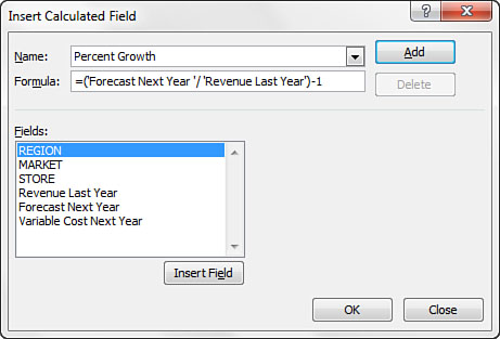
The next metric you need is percent growth over last year. To get this data, you need to add a calculated field that calculates the following formula:
(Forecast Next Year / Revenue Last Year) - 1
To accomplish this, do the following:
1. Activate the Insert Calculated Field dialog box and name your new field Percent Growth (see Figure 5.14).
Figure 5.14 Name your new field Percent Growth.
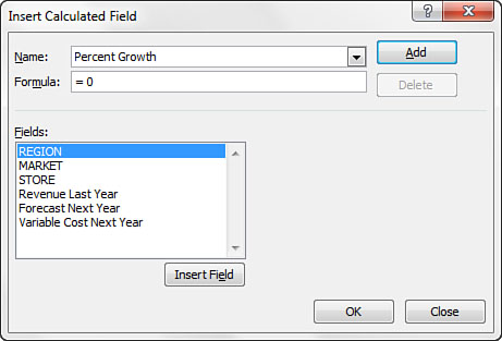
2. Delete the 0 in the Formula input box.
3. Enter ( (an open parenthesis).
4. Double-click the Forecast Next Year field.
6. Double-click the Revenue Last Year field.
7. Enter ) (a close parenthesis).
8. Enter - (a minus sign).
9. Enter the number 1.
Tip
You can use any constant in your pivot table calculations. Constants are static values that do not change. In this example, the number 1 is a constant. Though the value of Revenue Last Year or Forecast Next Year might change based on the available data, the number 1 will always have the same value.
After you have entered the full formula, your dialog box should look similar to the one shown in Figure 5.15.
Figure 5.15 With just a few clicks, you have created a variance formula!
With your formula typed in, you can click OK to add your new field. After changing the format of the resulting values to percent, you have a nicely formatted Percent Growth calculation in your pivot table. At this point, your pivot table should look like the one shown in Figure 5.16.
Figure 5.16 You have added a Percent Growth calculation to your pivot table.
With this newly created view into your data, you can see that three markets need to resubmit their forecasts to reflect positive growth over last year, as shown in Figure 5.17.
Figure 5.17 You can already discern some information from the calculated field that identifies three problem markets.

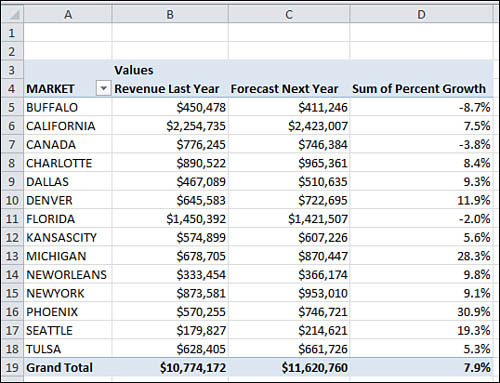
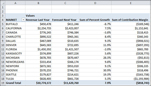
Now it is time to focus on your last requirement, which is to find total contribution margin by market. To get this data, you need to add a calculated field that calculates the following formula:
Forecast Next Year + Variable Cost Next Year
Note
A quick look at Figure 5.17 confirms that the Variable Cost Next Year field is not displayed in the pivot table report. Can you build pivot table formulas with fields that are not currently in the pivot table? The answer is yes. You can use any field that is available to you in the PivotTable Field List, even though that the field is not shown in the pivot table.
To create this field, do the following:
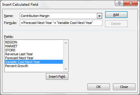
1. Activate the Insert Calculated Field dialog box and name your new field Contribution Margin.
2. Delete the 0 in the Formula input box.
3. Double-click the Forecast Next Year field.
4. Enter + (a plus sign).
5. Double-click the Variable Cost Next Year field.
After you have entered the full formula, your dialog box should look similar to the one shown in Figure 5.18.
Figure 5.18 With just a few clicks, you have created a formula that calculates contribution margin.
With the creation of the contribution margin, this report is ready to be delivered (see Figure 5.19).
Figure 5.19 Contribution margin is now a data field in your pivot table report thanks to your calculated field.
Now that you have built your pivot table report, you can analyze any new forecast submissions by refreshing your report with the new updates.
Creating Your First Calculated Item
As you learned at the beginning of this chapter, a calculated item is a virtual data item you create by executing a calculation against existing items within a data field. Calculated items come in especially handy when you need to group and aggregate a set of data items.
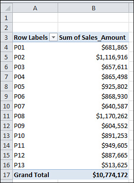
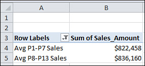
For example, the pivot table in Figure 5.20 gives you sales amount by Sales_Period. Imagine that you need to compare the average performance of the most recent six Sales_Periods to the average of the prior seven periods. In other words, you want to take the average of P01–P07 and compare it to the average of P08–P13.
Figure 5.20 You want to compare the most recent six Sales_Periods to the average of the prior seven periods.
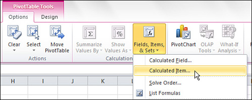
To do this, place your cursor on any data item in the Sales_Period field and then select Fields, Items & Sets from the Tools group. Next, select Calculated Item, as shown in Figure 5.21.
Figure 5.21 Start the creation of your calculated item by selecting Calculated Item.
Selecting this option opens the Insert Calculated Item dialog box. Figure 5.22 shows that the top of the dialog box identifies with which field you are working. In this case, it is the Sales_Period field. In addition, notice the Items list box is filled with all the items in the Sales_Period field automatically.
Figure 5.22 The Insert Calculated Item dialog box is populated to reflect the field with which you are working automatically.
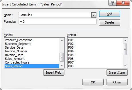
Your goal is to give your calculated item a name, and then build its formula by selecting the combination of data items and operators that provide the metric you are looking for.
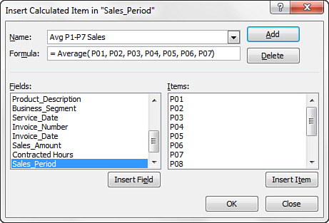
In this example, name your first calculated item Avg P1-P7 Sales, as shown in Figure 5.23.
Figure 5.23 Give calculated items descriptive names.

Next, you can build your formula in the Formula input box by selecting the appropriate data items from the Items list. In this scenario, you want to create the following formula:
= Average(P01, P02, P03, P04, P05, P06, P07)
Enter this formula into the Formula input box, as demonstrated in Figure 5.24.
Figure 5.24 Enter a formula that gives you the average of P01–P07.
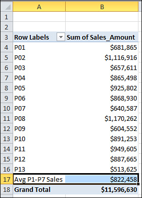
Click OK to activate your new calculated item. You now have a data item called Avg P1-P7 Sales, as shown in Figure 5.25.
Figure 5.25 A calculated item has been added successfully to your pivot table.
Tip
You can use any worksheet function in both a calculated field and a calculated item. The only restriction is that the function you use cannot reference external cells or named ranges. In effect, this means you can use any worksheet function that does not require cell references or defined names to work (such as COUNT, AVERAGE, IF, OR).
Create a calculated item to represent the average sales for P08–P13, as shown in Figure 5.26.
Figure 5.26 Create a second calculated item.

Now you can hide the individual sales periods, leaving only your two calculated items. After a little formatting, your calculated items enable you to compare the average performance of the six most recent Sales_Periods to the average of the prior seven periods (see Figure 5.27).
Figure 5.27 The most recent six Sales_Periods can be compared to the average of the prior seven periods.
Caution
If you do not hide the data items used to create your calculated item, your grand totals and subtotals might show incorrect amounts.
Understanding Rules and Shortcomings of Pivot Table Calculations
Although there is no better way to integrate your calculations into a pivot table than using calculated fields and calculated items, they come with their own set of drawbacks. It is important that you understand what goes on behind the scenes when you use pivot table calculations. It is even more important for you to be aware of the boundaries and limitations of calculated fields and calculated items to avoid potential errors in your data analysis.
The following sections highlight the rules around calculated fields and calculated items that you will most likely encounter when working with pivot table calculations.
Remembering the Order of Operator Precedence
Just as in a spreadsheet, you can use any operator in your calculation formulas, meaning any symbol that represents a calculation to perform (+, -, *, /, %, ^). Moreover, just as in a spreadsheet, calculations in a pivot table follow the order of operator precedence.
In other words, when you perform a calculation that combines several operators, as in (2+3) * 4/50%, Excel evaluates and performs the calculation in a specific order. Understanding the order of operations ensures that you avoid miscalculating your data.
The order of operations for Excel is as follows:
• Evaluate items in parentheses.
• Evaluate ranges (:).
• Evaluate intersections (spaces).
• Evaluate unions (,).
• Perform negation ([-]).
• Convert percentages (%).
• Perform exponentiation (^).
• Perform multiplication (*) and division (/), which are of equal precedence.
• Perform addition (+) and subtraction (-), which are of equal precedence.
• Evaluate text operators (&).
• Perform comparisons (=, <>, <=, >=).
Note
Operations that are equal in precedence are performed left to right.
Consider this basic example. The correct answer to (2+3)*4 is 20. However, if you leave off the parentheses, as in 2+3*4, Excel performs the calculation like this: 3*4 = 12 + 2 = 14. The order of operator precedence mandates that Excel perform multiplication before subtraction. Entering 2+3*4 gives you the wrong answer. Because Excel evaluates and performs all calculations in parentheses first, placing 2+3 inside parentheses ensures the correct answer.
Here is another widely demonstrated example. If you enter 10^2, which represents the exponent 10 to the 2nd power as a formula, Excel returns 100 as the answer. If you enter -10^2, you expect -100 to be the result. Instead, Excel returns 100 yet again. The reason is that Excel performs negation before exponentiation. This means that Excel converts 10 to -10 before the exponentiation, which effectively calculates -10*-10, which indeed equals 100. However, using parentheses in the formula, - (10^2), ensures that Excel calculates the exponent before negating the answer, which gives you -100.
Using Cell References and Named Ranges
When you create calculations in a pivot table, you are essentially working in a vacuum. The only data available to you is the data that exists in the pivot cache. Therefore, you cannot reach outside the confines of the pivot cache to reference cells or named ranges in your formula.
Using Worksheet Functions
You can use any worksheet function that does not require cell references or defined names as an argument. In effect, this means you can use any worksheet function that does not require cell references or defined names to work. Of the many functions that fall into this category, some include COUNT, AVERAGE, IF, AND, NOT, AND OR.
Using Constants
You can use any constant in your pivot table calculations. Constants are static values that do not change. For example, in the formula [Units Sold]*5, 5 is a constant. Though the value of Units Sold might change based on the available data, 5 will always have the same value.
Referencing Totals
Your calculation formulas cannot reference a pivot table’s subtotals or grand total. This means that you cannot use the result of a subtotal or grand total as a variable or argument in your calculated field.
Rules Specific to Calculated Fields
Calculated field calculations are always performed against the sum of your data. In basic terms, Excel always calculates data fields, subtotals, and grand totals before evaluating your calculated field. This means that your calculated field is always applied to the sum of the underlying data.
The example shown in Figure 5.28 demonstrates how this can adversely affect your data analysis.
Figure 5.28 Although the calculated field is correct for the individual data items in your pivot table, the subtotal is mathematically incorrect.
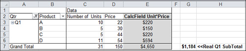
In each quarter, you need to get the total revenue for every product by multiplying the number of units sold by the price. If you look at Q1 first, you can immediately see the problem. Instead of returning the sum of 220+150+220+594, which would give you $1,184, the subtotal is calculating the sum of number of units times the sum of price, which returns the wrong answer.
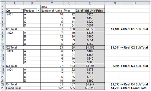
As you can see in Figure 5.29, including the whole year in your analysis compounds the problem.
Figure 5.29 The grand total for the year as a whole is completely wrong.
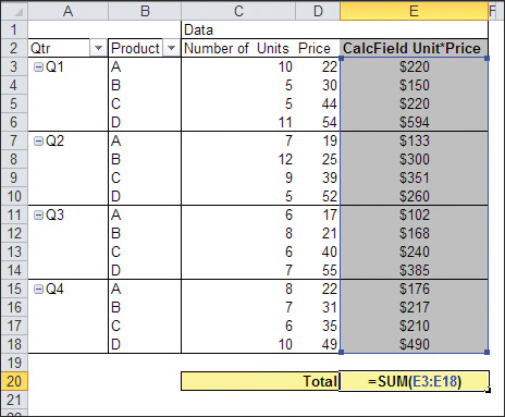
Tip
Unfortunately, there is no solution to this problem, but there is a workaround. In worst-case scenarios, you can configure your settings to eliminate subtotals and grand totals, and then calculate your own Totals. Figure 5.30 demonstrates this workaround.
Figure 5.30 Calculating your own totals can prevent reporting incorrect data.
Rules Specific to Calculated Items
You cannot use calculated items in a pivot table that uses averages, standard deviations, or variances. Conversely, you cannot use averages, standard deviations, or variances in a pivot table that contains a calculated item.
You cannot use a Report Filter field to create a calculated item, nor can you move any calculated item to the report filter area.
You cannot add a calculated item to a report that has a grouped field, nor can you group any field in a pivot table that contains a calculated item.
When building your calculated item formula, you cannot reference items from a field other than the one you are working with.
Note
As you think about the section you have just read, do not be put off by these shortcomings of pivot tables. Despite the clear limitations mentioned in this section, the capability to create custom calculations directly into your pivot table remains a powerful and practical feature that can enhance your data analysis. Now that you are aware of the inner workings of pivot table calculations and understand the limitations of calculated fields and items, you can avoid the pitfalls and use this feature with confidence.
Managing and Maintaining Pivot Table Calculations
In your dealings with pivot tables, you might find that sometimes you will not keep a pivot table for more than the time it takes to say, “Copy, Paste Values.” However, other times it can be more cost effective to keep your pivot table and all its functionality intact.
When you find yourself maintaining and managing your pivot tables through changing requirements and growing data, you might find the need to maintain and manage your calculated fields and calculated items.
Editing and Deleting Pivot Table Calculations
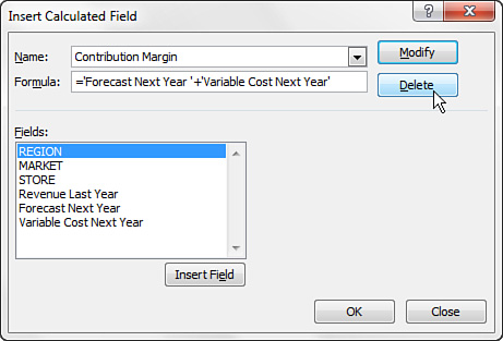
When your calculation’s parameters change or you no longer need your calculated field or calculated item, you can activate the appropriate dialog box to edit or remove the calculation.
To do this, activate the Insert Calculated Field or Insert Calculated Item dialog box and select the Name drop-down, as shown in Figure 5.31.
Figure 5.31 Opening the drop-down list under Name reveals all the calculated fields or items in the pivot table.
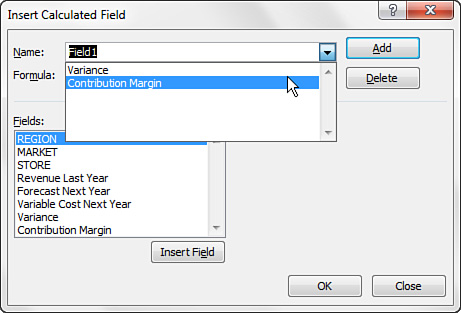
After you select a calculated field or item, you have the option of deleting the calculation or modifying the formula, as shown in Figure 5.32.
Figure 5.32 After selecting the appropriate calculated field or item, you can either delete or modify the calculation.
Changing the Solve Order of Calculated Items
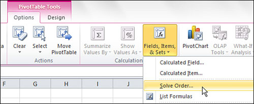
If the value of a cell in your pivot table is dependent on the results of two or more calculated items, you have the option to change the solve order of the calculated items. In other words, you can specify the order in which the individual calculations are performed.
To get to the Solve Order dialog box, place your cursor anywhere in the pivot table, select Fields, Items, & Sets from the Tools group, and then select Solve Order, as shown in Figure 5.33.
Figure 5.33 Activate the Solve Order dialog box by selecting Formulas and then Solve Order.
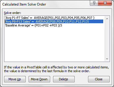
The Solve Order dialog box lists all the calculated items that currently exist in your pivot table (see Figure 5.34). Select any of the calculated items you see listed to enable the Move Up, Move Down, and Delete command buttons. The order you see the formulas in this list is the exact order the pivot table performs each operation.
Figure 5.34 After identifying the calculated item you are working with, move the item up or down to change the solve order. You also have the option of deleting the item in this dialog box.
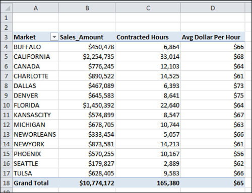
Documenting Formulas
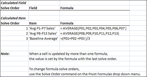
Excel provides a nice function that lists the calculated fields and calculated items used in your pivot table. This function can also provide details of the solve order and formulas. This feature comes in especially handy when you need to determine which calculations are applied in a pivot table and the fields or items those calculations affect.
To use this function to list your pivot table calculations, place your cursor anywhere in the pivot table to select Fields, Items, & Sets, and then select List Formulas. Excel creates a new tab in your workbook that lists the calculated fields and calculated items in the current pivot table. Figure 5.35 shows a sample output of the List Formulas command.
Figure 5.35 The List Formulas command enables you to document the details of your pivot table calculations quickly.
Next Steps
In the next chapter, you learn the fundamentals of pivot charts and the basics of representing your pivot data graphically. You also gain a firm understanding of the limitations of pivot charts and alternatives to using pivot charts.