Introduction
Pivot tables are the single most powerful command in all of Excel. They came along during the 1990s when Microsoft and Lotus were locked in a bitter battle for dominance of the spreadsheet market. The race to continually add enhanced features to their respective products during the mid-1990s led to many incredible features, but none as powerful as the pivot table.
With a pivot table, you can take 1 million rows of transactional data and transform it into a summary report in seconds. If you can drag a mouse, you can create a pivot table. In addition to quickly summarizing and calculating data, pivot tables allow you to change your analysis on the fly by simply moving fields from one area of a report to another.
No other tool in Excel gives you the flexibility and analytical power of pivot tables.
What You Will Learn from This Book
It is widely agreed that close to 50 percent of Excel users leave 80 percent of Excel untouched. That is, most users do not tap into the full potential of Excel’s built-in utilities. Of these utilities, the most prolific by far is the pivot table. Despite the fact that pivot tables have been a cornerstone of Excel for more than 15 years, they remain one of the most underutilized tools in the entire Microsoft Office Suite. Having picked up this book, you are savvy enough to have heard of pivot tables or even have used them on occasion. You have a sense that pivot tables have a power that you are not using, and you want to learn how to leverage that power to increase your productivity quickly.
Within the first two chapters, you will be able to create basic pivot tables, increase your productivity, and produce reports in minutes instead of hours. Within the first seven chapters, you will be able to output complex pivot reports with drill-down capabilities accompanying charts. By the end of the book, you will be able to build a dynamic pivot table reporting system.
What Is New in Excel 2010’s Pivot Tables
Excel 2010 introduces three new features designed to solve common problems with pivot tables. Combined with the two items added to Excel 2007, you have five great improvements to pivot tables.
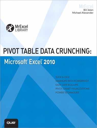
• Beginning in Excel 2007, multiple items could be selected from the filter drop-down. However, this feature left behind a confusing report because the filters section left the ambiguous words “(Multiple Items)” to explain which items are included in the filter. As shown in Figure I.1, the new Excel 2010 Slicers feature provides a graphical view of which items are selected for the pivot table. Read more about Slicers in Chapter 4, “Grouping, Sorting, and Filtering Pivot Data.”
Figure I.1 Slicers visually show which items are included in a filter.
• In legacy versions of Excel, one of the many calculation options available in pivot tables has been “Percentage of Column.” This feature was fine when you had only one field along the left side of the pivot table. However, if you had two or more fields, you might want to show the percentage of the next subtotal. In Excel 2010, Microsoft added new calculation options including % of Parent and Rank. Calculation options are discussed in Chapter 3, “Customizing a Pivot Table.”
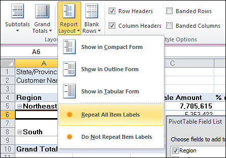
• A constant annoyance is the blank cells included in the outermost column fields. For an example, see A6:A7 in Figure I.1. At last, Excel 2010 offers the Design, Report Layout, Repeat All Item Labels to fill in those blank cells.
• PowerPivot is a free add-in from Microsoft that allows you to create pivot tables from external data or from separate sheets.
• If you skipped Excel 2007, you notice that the Pivot Table Field List has been expanded. Rather than dragging fields to drop zones on the pivot table itself, beginning with Excel 2007, you drag the fields to the drop zones in the pivot table field list. Excel 2007 also added filtering options.
Skills Required to Use This Book
We have created a reference that is comprehensive enough for hard-core analysts yet relevant to casual users of Excel. The bulk of the book covers how to use pivot tables in the Excel user interface. The final chapter describes how to create pivot tables in Excel’s powerful VBA macro language. This means that any user who has a firm grasp of basics, such as preparing data, copying, pasting, and entering simple formulas, should not have a problem understanding the concepts in this book.
Case Study: Life Before Pivot Tables
Imagine that it is 1992 and you are using Lotus 1-2-3 or Excel 4. You have thousands of rows of transactional data. Your manager asks you to prepare a summary report showing revenue by region and product. The following case study walks you through how this report would have been prepared in 1992.
In 1992, preparing this report was a daunting task. It required superhuman spreadsheet skills that few could master. Here are the steps you needed to take to prepare a summary report showing revenue by region and product:
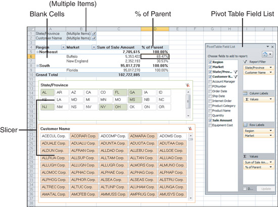
1. You need to get a list of the unique regions in the data set. Use the Advanced Filter command with Unique Records Only to extract a list of the unique regions (see Figure I.2).
Figure I.2 Even today, the Advanced Filter command is not a lot of fun to use.
2. You also need to get a list of the unique products in the data set. Use the Advanced Filter command with Unique Records Only a second time to extract a list of the unique products.
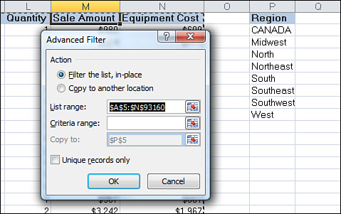
3. Turn the list of regions sideways so that it runs across the columns. Copy the list of unique regions. Then select Edit, Paste Special, Transpose to arrange the regions as headings going across the report. You now have a skeleton of the report, as shown in Figure I.3.
Figure I.3 After using a second Advanced Filter command and selecting Edit, Paste Special, Transpose, you have this skeleton of the final report. You still have a long way to go.
4. Next, you need to build a DSUM formula to get total Sales for one product and region. DSUM requires that you build a criteria range as shown in R1:S2 in Figure I.4.
Figure I.4 Use the ancient DSUM function with a four-cell criteria range.
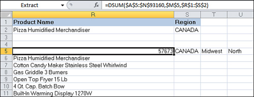
5. In the corner cell of the report, build the formula to get total sales for the selected product and region: =DSUM($A$5:$N$93160,$M$5,$R$1:$S$2). This is a formula to test whether the region column is Canada and if the product is a Pizza Merchandiser.
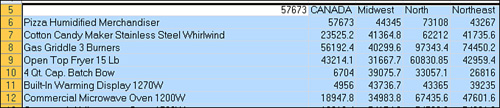
6. You are a long-time, hard-core data analyst if you remember pressing the keystrokes for /Data Table 2 in Lotus 1-2-3. Figure I.5 shows the equivalent function in Excel. In Excel 2010, this command is found in Data, Data Tools, What If Analysis, Data Table.
Figure I.5 The Data Table command replicates the formula in the top-left corner of the table, but replaces two references in the formula with the headings at the top and left of the report.

7. Finally, after using two advanced filters and a Paste Tranpose command, writing an obscure DSUM formula, and then using the Data Table command, you have the result your manager is looking for, as shown in Figure I.6. If you could pull off this analysis in 10 minutes, you were doing an amazing job.
Figure I.6 After displaying knowledge of obscure spreadsheet commands in 10 minutes, you have produced the needed report.
Now, if your manager looks at the report and asks you to add Market to the analysis, you are nearly back at square one because it will take an additional 10 minutes to produce the new report.
Invention of the Pivot Table
The concept that led to today’s pivot table came from the halls of the Lotus Development Corporation with a revolutionary spreadsheet program called Lotus Improv. Improv was envisioned in 1986 by Pito Salas of the Advanced Technology Group at Lotus (see Figure I.7). Realizing that spreadsheets often have patterns of data, Salas concluded that if a user could build a tool that could recognize these patterns, then he could build enhanced data models. Lotus ran with the concept and started developing the next-generation spreadsheet.
Figure I.7 Salas, inventor of the pivot table concept, is always working on cutting-edge products at www.salas.com.

Throughout 1987, Lotus demonstrated its new program to a few companies. In 1988, Steve Jobs saw the program and immediately wanted it developed for his upcoming NeXT computer platform. The program, finally named Lotus Improv, was eventually shipped in 1991 for the NeXT platform. A version for Windows was introduced in 1993.
The core concept behind Improv was that data, data views, and formulas should be encapsulated as separate entities and treated as different animals. For the first time in a spreadsheet program, a data set was given a name that could be grouped into larger categories. This naming and grouping capability paved the way for the most powerful feature in Improv: rearranging data. With Improv, a user could define and store a set of categories and then change the view by simply dragging the category names with the mouse. The user could also create totals and group summaries.
Microsoft eventually incorporated this concept in its pivot table functionality in Excel 5. Years later, with the release of Excel 97, Microsoft offered users an enhanced pivot table wizard and key improvements to pivot table functionality such as the capability to add calculated fields. Excel 97 also opened the pivot cache to developers, fundamentally changing the way pivot tables are created and managed. Microsoft introduced the pivot chart with Excel 2000, providing users a way to represent pivot tables graphically. Excel 2002 added the GetPivotData function. Excel 2007 added new filters such as selecting dates in the “last quarter” or “this year.” Excel 2010 continues improving pivot tables with new features described previously.
Case Study: Life After Pivot Tables
Say you have 100,000 rows of transactional data, as discussed in the previous case study. Your manager asks you to prepare a summary report showing revenue by Region and Product. Fortunately, you have pivot tables at your disposal. Here are the steps you would follow today using Excel 2010:
1. Select a single cell in your data set. Select PivotTable from the Insert tab. Click OK. You are given a blank pivot table, as shown in Figure I.8.
Figure I.8 After three mouse clicks, you have a blank pivot table report. Three more mouse clicks to go.

2. From the Pivot Table Field List, select the Product Name check box. Excel adds a unique list of products to the left side of the pivot table. Select the Sale Amount check box. Excel adds total sales by product to the report. Click the Region field in the Field List and drag it to the Column Labels drop zone. After six mouse clicks, you have the required report, as shown in Figure I.9.
Figure I.9 Add three fields to the report.
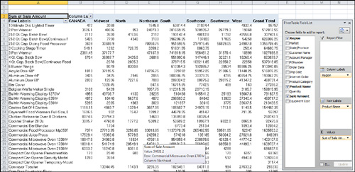
If you are racing, you can actually create the report shown in Figure I.9 in exactly 10 seconds. This is an amazing accomplishment. Realistically, it would take you about 50 seconds at normal speed to create the report. If you are a spreadsheet wizard following the steps in the previous case study, the nonpivot table solution would take you at least 12 times longer.
![]() To see the creation of a pivot table, search for Pivot Table Data Crunching Intro at YouTube.
To see the creation of a pivot table, search for Pivot Table Data Crunching Intro at YouTube.
In addition, when your manager comes back with the request to add Market to the analysis, you need just seconds to drag the Market field to the Column Labels drop zone in the PivotTable Field List to add it to the report, as shown in Figure I.10.
Figure I.10 To create a new report with the Market field, simply drag the field to a drop zone.

Sample Files Used in This Book
All data files used throughout this book are available for download from www.mrexcel.com/pivotbookdata2010.html.
Conventions Used in This Book
This book follows certain conventions:
• Monospace—Text messages you see onscreen or code that appears in a monospace font.
• Bold Monospace—Text you type appears in a bold, monospace font.
• Italic—New and important terms appear in italics.
• Initial Caps—Tab names, dialog box names, and dialog box elements are presented with initial capital letters so you can identify them easily.
Referring to Versions
From 1997 through 2003, Microsoft released similar versions of Excel known as Excel 97, Excel 2000, Excel 2002/XP, and Excel 2003. This book will refer to those versions as “legacy versions” of Excel.
Referring to Ribbon Commands
Office 2007 introduced a new interface called the Ribbon. The Ribbon is composed of several tabs labeled Home, Insert, Page Layout, and so on. When you click on the Page Layout tab, you see the icons available on the Page Layout tab.
When the active cell is inside a pivot table, two new tabs appear on the Ribbon. In the help files, Microsoft calls these tabs “PivotTable Tools, Options” and “PivotTable Tools, Design.” For convenience, this book refers to these elements as the Options tab and the Design tab, respectively. The new Slicer feature introduces a new Ribbon tab that Microsoft calls “Slicer Tools, Options.” This book refers to this as the Slicer tab.
In some cases, the Ribbon icon leads to a drop-down with additional choices. In these cases, the book lists the hierarchy of Ribbon, Icon, Menu Choice, and Submenu Choice. For example, in Figure I.11, the shorthand specifies “Select Design, Report Layout, Repeat All Item Labels.”.
Figure I.11 For shorthand, instructions might say Select Design, Report Layout, Repear All Item Labels.
Special Elements
This book contains the following special elements:
![]() Some topics will be demonstrated in a short video cast at YouTube.
Some topics will be demonstrated in a short video cast at YouTube.
Note
Notes provide additional information outside the main thread of the chapter discussion that might be useful for you to know.
Tip
Tips provide you with quick workarounds and time-saving techniques to help you do your work more efficiently.
Caution
Cautions warn you about potential pitfalls you might encounter. Pay attention to Cautions because they alert you to problems that otherwise could cause you hours of frustration.