
Worked Example 3
Motor Car
Chapter Outline
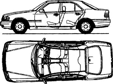
The example in this chapter shows how all the tools and techniques described so far can be integrated to give a comprehensive project management system. The project chosen is the design, manufacture, and distribution of a prototype motor car and while the operations and time scales are only indicative and do not purport to represent a real-life situation, the examples show how the techniques follow each other in a logical sequence.
The prototype motor car being produced is illustrated in Figure 49.1 and the main components of the engine are shown in Figure 49.2. It will be seen that the letters given to the engine components are the activity identity letters used in planning networks.

The following gives an oversight of the main techniques and their most important constituents.
As with all projects, the first document to be produced is the Business Case, which should also include the chosen option investigated for the Investment Appraisal. In this exercise, the questions to be asked (and answered) are shown in Table 49.1.
It is assumed that the project requires an initial investment of ≤60 million and that over a five-year period, 60,000 cars (units) will be produced at a cost of ≤5000 per unit. The assumptions are that the discount rate is 8%. There are two options for phasing the manufacture:
(a) That the factory performs well for the first two years but suffers some production problems in the next three years (option 1); and
(b) That the factory has teething problems in the first three years but goes into full production in the last two (option 2).
The Discounted Cash Flow (DCF) calculations can be produced for both options as shown in Tables 49.2 and 49.3.
Table 49.2
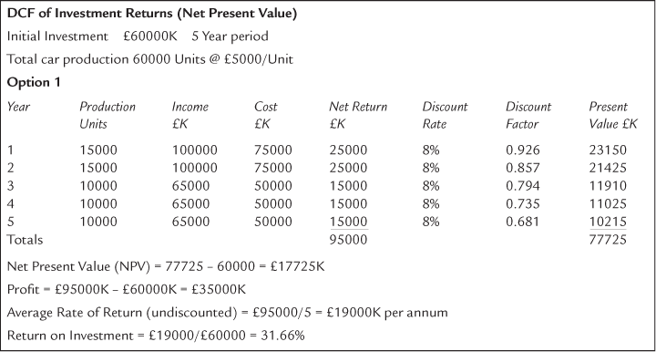
Table 49.3

To obtain the Internal Rate of Return (IRR), an additional discount rate (in this case 20%) must be applied to both options. The resulting calculations are shown in Tables 49.4 and 49.5 and the graph showing both options is shown in Figure 49.3. This gives an IRR of 20.2% and 15.4%, respectively.
Table 49.4
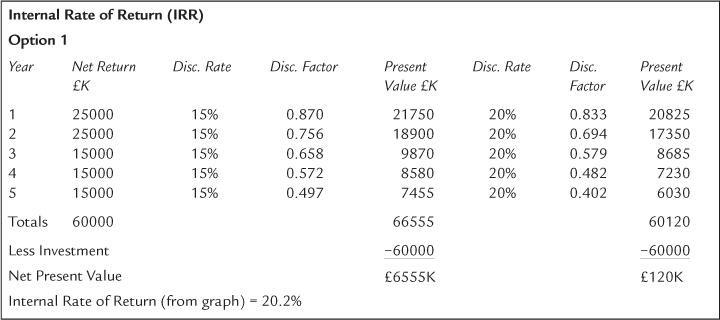
Table 49.5


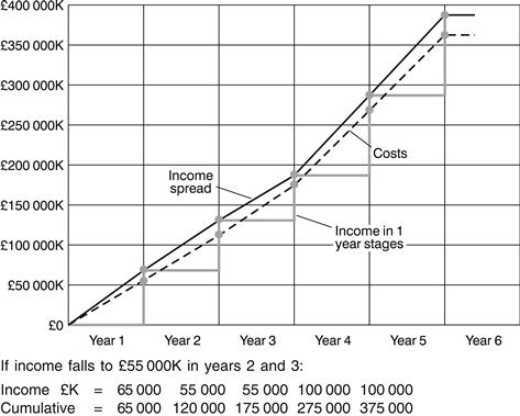
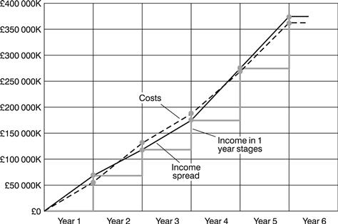
It is now necessary to carry out a cash flow calculation for the distribution phase of the cars. To line up with the DCF calculations, two options have to be examined. These are shown in Tables 49.6 and 49.7 and the graphs in Figures 49.4 and 49.5 for option 1 and option 2, respectively. An additional option 2a in which the income in years 2 and 3 is reduced from ≤65000K to ≤55000K is shown in the cash flow curves of Figure 49.6.
Table 49.6
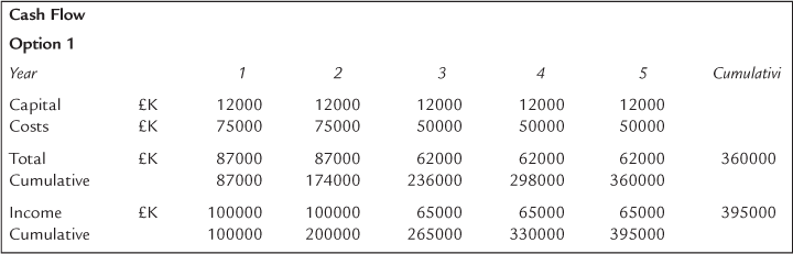
Table 49.7


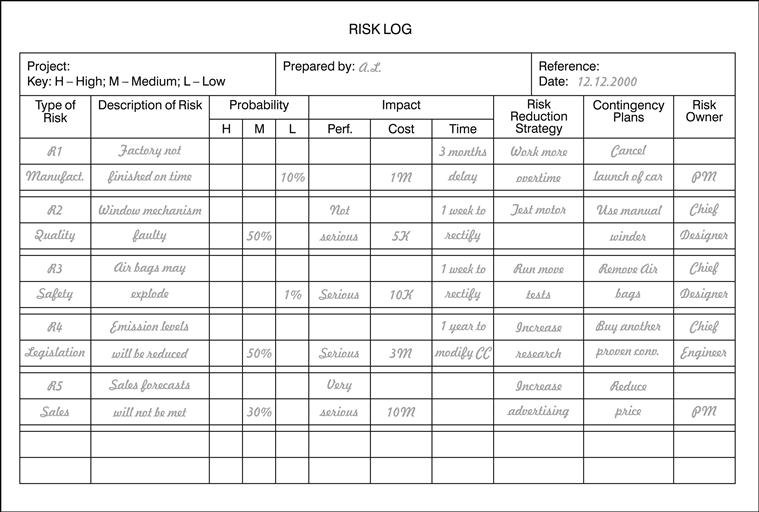
All projects carry an element of Risk and it is prudent to carry out a risk analysis at this stage. The types of risks that can be encountered, the possible actual risks, and the mitigation strategies are shown in Table 49.8. A risk log (or risk register) for five risks is given in Figure 49.7.
Table 49.8
| Risk Analysis | Training problems |
| Types of risks | Suppliers unreliable |
| Manufacturing (machinery and facilities) costs | Rustproofing problems |
| Sales and marketing, exchange rates | Performance problems |
| Reliability | Industrial disputes |
| Mechanical components performance | Electrical and electronic problems |
| Electrical components performance | Competition too great |
| Maintenance | Not ready for launch date (exhibition) |
| Legislation (emissions, safety, recycling, labour, tax) | Safety requirements |
| Quality | Currency fluctuations |
| Possible risks | Mitigation strategy |
| Won’t sell in predicted numbers | Overtime |
| Quality in design, manufacture, finish | More tests |
| Maintenance costs | More research |
| Manufacturing costs | More advertising/marketing |
| New factory costs | Insurance |
| Tooling costs | Re-engineering |
| New factory not finished on time | Contingency |
Once the decision has been made to proceed with the project, a Project Life Cycle diagram can be produced. This is shown on Figure 49.8 together with the constituents of the seven phases envisaged.
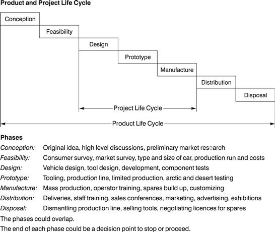
Figure 49.8
The next stage is the Product Breakdown Structure (Figure 49.9), followed by a combined Cost Breakdown Structure and Organization Breakdown Structure (Figure 49.10). By using these two, the Responsibility Matrix can be drawn up (Figure 49.11).

Figure 49.9

Figure 49.10

Figure 49.11
It is now necessary to produce a programme. The first step is to draw an Activity List showing the activities and their dependencies and durations. These are shown in the first four columns of Table 49.9. It is now possible to draw the Critical Path Network in either AoN format (Figure 49.12), AoA format (Figure 49.13), or as a Lester diagram (Figure 49.14).

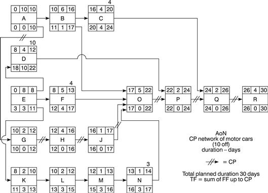
Figure 49.12

Figure 49.13
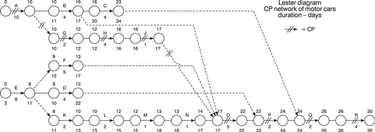
Figure 49.14
After analysing the network diagram, the Total Floats and Free Floats of the activities can be listed (Table 49.10).

Apart from the start and finish, there are four milestones (days 8, 16, 24, and 30). These are described and plotted on the Milestone Slip Chart (Figure 49.15).

Figure 49.15
The network programme can now be converted into a bar chart (Figure 49.16) on which the resources (in men per day) as given in the fifth column of Table 49.9 can be added. After summating the resources for every day, it has been noticed that there is a peak requirement of 12 men in days 11 and 12. As this might be more than the available resources, the bar chart can be adjusted by utilizing the available floats to smooth the resources and eliminate the peak demand. This is shown in Figure 49.17 by delaying the start of activities D and F.


In Figure 49.18, the man days of the unsmoothed bar chart have been multiplied by 8 to convert them into manhours. This was necessary to carry out Earned Value Analysis. The daily manhour totals can be shown as a histogram and the cumulative totals are shown as an ‘S’ curve. In a similar way Figure 49.19 shows the respective histogram and ‘S’ curve for the smoothed bar chart.

Figure 49.18
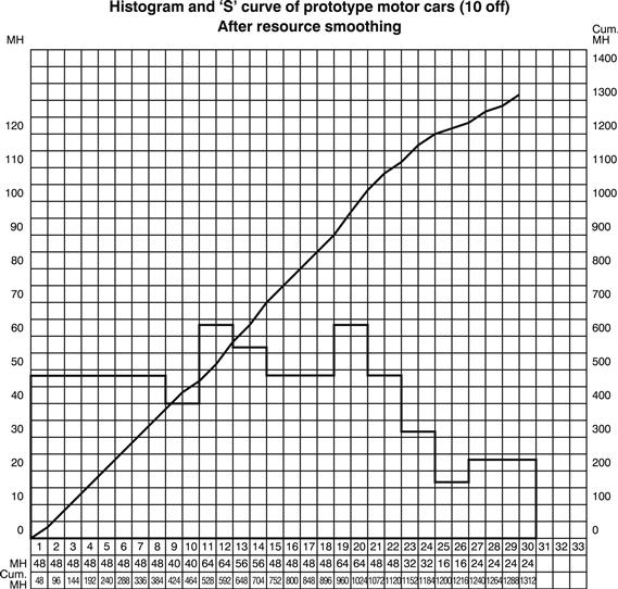
Figure 49.19
It is now possible to draw up a table of Actual Manhour usage and % complete assessment for reporting day nos. 8, 16, 24, and 30. These, together with the Earned Values for these periods are shown in Table 49.11. Also shown are the efficiency (CPI), SPI, and predicted final completion costs and times as calculated at each reporting day.

Using the unsmoothed bar chart histogram and ‘S’ curve as a Planned man hour base, the Actual manhours and Earned Value manhours can be plotted on the graph in Figure 49.20. This graph also shows the % complete and % efficiency at each of the four reporting days.

Finally, Table 49.12 shows the actions required for the Close-Out procedure.
Summary
Business Case
Need for new model. What type of car? Min./max. price. Manufacturing cost. Units per year.Marketing strategy. What market sector is it aimed at? Main specification. What extras should be standard? Name of new model. Country of manufacture.
Investment Appraisal
Options: Saloon, Coupé, Estate, Convertible, People carrier, 4 × 4. Existing or new engine. Existing or new platform. Materials of construction for engine, body. Type of fuel. New or existing plant. DCF of returns, NPV, Cash flow.
Project and Product Life Cycle
| Conception: | Original idea, submission to top management |
| Feasibility: | Feasibility study, preliminary costs, market survey |
| Design: | Vehicle and tool design, component tests |
| Prototype: | Tooling, production line, environmental tests |
| Manufacture: | Mass production, training |
| Distribution: | Deliveries, staff training, marketing |
| Disposal: | Dismantling of plant, selling tools |
Work and Product Breakdown Structure
Design, Prototype, Manufacture, Testing, Marketing, Distribution, Training.
Body, Chassis, Engine, Transmission, Interior, Electronics.
Cost Breakdown Structure, Organization Breakdown Structure, Responsibility Matrix.
AoN Network
Network diagram, forward and backward pass, floats, critical path, examination for overall time reduction, conversion to bar chart with resource loading, histogram, reduction of resource peaks, cumulative ‘S’ curve. Milestone slip chart.
Risk Register
Types of risks: manufacturing, sales, marketing, reliability, components failure, maintenance, suppliers, legislation, quality. Qualitative and quantitative analysis. Probability and impact matrix. Risk owner. Mitigation strategy, contingency.
Earned Value Analysis
EVA of manufacture and assembly of engine, calculate Earned Value, CPI, SPI, cost at completion, final project time, draw curves of budget hours, planned hours, actual hours earned value, % complete, efficiency over four reporting periods.
Close-Out
Close-out meeting
Close-out report
Instruction manuals
Test certificates
Spares lists
Dispose of surplus materials