
4 2. DYNAMIC MODEL OF VEHICLE ROLLOVER
CG
m
s
a
y
m
s
a
y
m
s
g
m
s
g
t
w
H
CG,s
H
RC
K
ϕ
j
F
z,RC
F
y,RC
d
CG
RC
RC
ϕ
ϕ
B
ϕ
B
ϕ
S
Z
Y
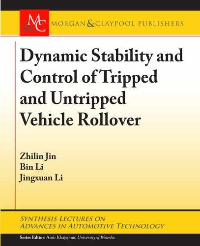
Figure 2.1: Schematic representation of suspended roll plane model.
g is the acceleration of gravity; H
CG;s
is the CG height of sprung mass respect to grand; H
RC
is the height of roll axis respect to grand; K
is the roll stiffness of suspension; M
RC
is the roll
moment, measured about roll center; m
s
is the sprung mass; is the total roll angle of vehicle;
and
B
is the road bank angle.
By the roll plane model, a threshold used to determine the degree of rollover can be de-
rived. is model can also be used to design the rollover control strategy.
2.2 YAW-ROLL MODEL
ere are many factors that cause the vehicle to roll over. Since it only considers the influence
of roll motion on the rollover, the roll model has some limitations. Some researchers consider
the yaw motion on the basis of the roll plane model. Yu established a yaw-roll model for heavy-
duty vehicle and designed a prototype active roll control system [6]. Chen also used simplified
yaw-roll model to compute a Time-To-Rollover index and then corrected it using an Artificial
Neural Network [7]. As can be seen from Figure 2.2, the proposed yaw-roll model is separated
into a yaw and a roll part. is serial arrangement may have less accurate results compared with
an integrated yaw-roll model. However, this simplified structure was found to be superior in
two aspects: (1) ease of model construction and (2) faster computations.

2.2. YAW-ROLL MODEL 5
Yaw
Model
S
teering
Angle
Lateral
Acceleration
Roll Angle
Roll Rate
Roll
Model
Figure 2.2: Structure of the simplified yaw-roll model.
As shown in Figure 2.3, the vehicle yaw model was assumed to be described by a linear
bicycle model and the vehicle speed is assumed to be constant.
Yaw Rate, r Lo
ngitudinal
Velocity, u
Lateral
Velocity, v
Acceleration, ay
Tire Steering
Angle, δ
tire
Figure 2.3: Yaw model.
For a linear bicycle model, the discrete-time transfer function from the steering angle to
lateral acceleration is known to have the following form:
T
yaw
.z/ D
b
0
z
2
C b
1
z C b
2
z
2
C a
1
z C a
2
D
a
y
ı
; (2.7)
where a
y
is the lateral acceleration and ı is the steering wheel angle which is related to the tire
steering angle by a steering gear ratio. After factorization, we can get the following form:
T
yaw
.z/ D b
0
C k
z z
1
.z p
1
/.z Np
1
/
; (2.8)
where k, z
1
, p
1
, and p
2
can be calculated by standard system identification techniques and then
take the average of their values for multiple files of the same maneuver. ese transfer functions
have been found to work well under constant speed cases.
e roll model was found to be well behaved which is a 2-degree-of-freedom (DOF)
model (sprung mass roll and unsprung mass roll, refer to Figure 2.4).
e structure of the discrete-time transfer fiction from lateral acceleration to sprung mass
roll angle is shown as follows:
T
roll
.z/ D
b
0
z
3
C b
1
z
2
C b
2
z C b
3
z
4
C a
1
z
3
C a
2
z
2
C a
3
z C a
4
D
a
y
; (2.9)
where is the roll angle of the sprung mass.
..................Content has been hidden....................
You can't read the all page of ebook, please click here login for view all page.