CHAPTER
13

Common Derivative Applications

In This Chapter

• Approximating zeroes of functions
• Limits of indeterminate expressions
• The Mean Value Theorem
• Rolle’s Theorem
• Calculating related rates
• Maximizing and minimizing functions

It’s been a fun ride, but our time with the derivative is almost through. Don’t get too emotional yet—I’ve saved the best for last, and this chapter will be a hoot (if you like word problems, that is). As in the last chapter, we’ll be looking at the relationship between calculus and the real world, and you’ll probably be surprised by what you can do with very simple calculus procedures.

This chapter has it all: cool shortcuts, a few more existence theorems, romance, adventure, and the two topics most first-year calculus students find the trickiest. We’ll go through the topics in the order of difficulty, starting with the easiest and progressing to the more advanced.

Newton’s Method

You may remember that Sir Isaac Newton was one of the two men responsible for discovering/inventing calculus. One technique named for him allows you to approximate difficult-to-find roots (or zeroes) of a function.

This technique is interesting mostly because of its historic significance rather than its modern-day usefulness. Back in Chapter 10 you learned how to use your calculator to approximate difficult roots, rather than churning them out by hand.

You may be interested to know that your calculator uses a technique very similar to Newton’s Method to calculate those roots, and after spending a few moments working with it, you may gain an appreciation for all the work your calculator is doing behind the scenes.

Newton’s Method is an iterative formula that can be repeated over and over, each time producing a value that is slightly closer to the correct answer (if everything is working correctly). You begin with a seed value, something relatively close to the right answer (like the guesses your calculator required in Chapter 10). Often, that seed value is called x₀, and after running it through the formula you end up with a better guess called x₁. You can then run x₁ through the formula to get an even better guess called x₂ and so on.

With this in mind, Newton’s Method calls your current guess x_n and the resulting better guess x_n + 1. To generate that better guess you apply this formula:

In other words, from your original guess x_n, you subtract the function evaluated at x_n divided by the derivative of the function evaluated at x_n.

Example 1: Calculate two iterations of Newton’s Method to approximate the positive root of f(x) = x² – 5 using an initial (seed) value of x₀ = 2.

Solution: Look at the graph of f(x) in Figure 13.1. It appears to cross the x-axis at a value slightly greater than 2 and a value slightly less than –2. The problem asks you to estimate the positive root, so the seed value of x₀ = 2 seems like a good guess to begin with.

Figure 13.1

The graph of f(x) = x2 – 5.

Begin by evaluating the function and its derivative, f ′(x) = 2x, at the seed value, x₀ = 2:

f(2) = 2² – 5 = –1                             f ′(2) = 2 ∙ 2 = 4

Substitute these values into Newton’s Method to calculate x_{n + 1} = x_{0 + 1} = x₁:

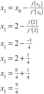
According to Newton’s Method, is a better estimate of the positive root of f(x) than the original guess of x₀ = 2. For an even better guess, substitute into Newton’s Method to calculate x₂:

Time out! These fractions are getting ugly, and they only get uglier with every iteration. I think it’s time to cut our losses and type this into a calculator to finish:

After two iterations of Newton’s Method, you have calculated an estimated root of 2.23611 for f(x). You could go on, getting closer and closer to the root, but I think we all have better things to do.

Evaluating Limits: L’Hôpital’s Rule

Way, way back, many chapters ago, in a galaxy far, far away, you were stressed about limits. Since then, you’ve had a whole lot more to stress about, so it’s high time we destressed you a bit. Little did you know that as you were plugging away, learning derivatives, you also learned a terrific shortcut for finding limits. This shortcut (called L’Hôpital’s Rule) can be used to find limits that, after substitution, are in indeterminate form.

To show just how useful L’Hôpital’s Rule is, we’ll return briefly to Chapter 6 and fish out two limits we couldn’t previously calculate by hand. These two limits will comprise the next example. The first limit we could only memorize (but couldn’t justify via any of our methods at the time). We calculated the second limit using a little trick (comparing degrees for limits at infinity), but that method was a trick only. We had no proof or justification for it at all. Finally, a little pay dirt for the curious at heart.

L’Hôpital’s Rule: If and is in indeterminate form (e.g., ), then . In other words, take the derivatives of the numerator and denominator separately (not via the Quotient Rule) and substitute in c gain to find the limit.

Example 2: Calculate both of the following limits using L’Hôpital’s Rule:

(a)

Solution: If you substitute in x = 0, you get , which is in indeterminate form. So apply L’Hôpital’s Rule by taking the derivative of sin x (which is cos x) and the derivative of x (which is 1) and replacing those pieces with their derivatives:

Now the substitution method won’t give you . In fact, substituting gives you cos 0, which equals 1. You learned that 1 was the answer in Chapter 6, but now you know why.

(b)

Solution: If you plug in x = ∞ for all the x’s you get a huge number on top divided by a huge number on the bottom, or , which is in indeterminate form. Apply L’Hôpital’s Rule:

Uh-oh. Substitution still gives you . Never fear! Keep applying L’Hôpital’s Rule until substituting gives you a nonindeterminate answer:

Once there are no more x’s in the problem, no substitution is necessary, and the answer falls out like a ripe fruit.

You might remember this problem—it was Example 6 in Chapter 6. You used a different method to compute the limit then, but you got the same answer: .

More Existence Theorems

Man has struggled for centuries to define life and to determine what, exactly, defines existence. Descartes once mused, “I think; therefore, I am,” suggesting that thought defined existence. Most calculus students go one step further, lamenting, “I am in mental anguish; therefore, I am in calculus.” Philosophy aside, the next two theorems don’t try to answer such deep questions; they simply state that something exists, and that’s good enough for them.

The Mean Value Theorem

This neat little theorem gives an explicit relationship between the average rate of change of a function (i.e., the slope of a secant line) and the instantaneous rate of change of a function (i.e., the slope of a tangent line). Specifically, it guarantees that at some point on a closed interval, the tangent line will be parallel to the secant line for that interval (see Figure 13.2).

Figure 13.2

Here, the secant line is drawn connecting the endpoints of the closed interval [a,b], at x = c, which is on that interval; the tangent line is parallel to the secant line.

Mathematically, parallel lines have equal slopes. Therefore, there is always some place on an interval where a continuous function is changing at exactly the same rate it’s changing on average for the entire interval. Here’s the theorem in math jibber jabber:

The Mean Value Theorem: If a function f(x) is continuous and differentiable on the closed interval [a,b], then there exists a value c between a and b such that . In other words, a value c is guaranteed to exist such that the derivative there (f′(c)) is equal to the slope of the secant line for the interval [a,b] .

Example 3: At what x-value(s) on the interval [–2,3] does the graph of f(x) = x² + 2x – 1 satisfy the Mean Value Theorem?

Solution: The function is continuous and differentiable because there are no domain restrictions. Somewhere, the derivative must equal the secant slope, so start by finding the derivative of f(x):

f′(x) = 2x + 2

That was easy. Now find the secant slope over the interval [–2,3]. To calculate it, first plug –2 and 3 into the function to get the secant’s endpoints, (–2,–1) and (3,14):

Therefore, at some point on the interval, the derivative, f′(x) = 2x + 2, and the secant slope you calculated, 3, must be equal:

Look at the graph of f(x) in Figure 13.3 to verify that the tangent line at is parallel to the secant line connecting (–2,–1) and (3,14).

Figure 13.3

Equal secant and tangent slopes result in parallel secant and tangent lines.

Rolle’s Theorem

Rolle’s Theorem is a specific case of the Mean Value Theorem. It says that if the slope of a function’s secant line is 0 (in other words, the secant line is horizontal because the endpoints of the interval are located at the exact same height on the graph), then somewhere on that interval, the tangent slope will also be 0. Because you already understand the Mean Value Theorem, this isn’t new information. Our previous theorem guaranteed the lines would have the same slope no matter what the secant slope was. Here’s how Rolle’s Theorem is defined mathematically:

Rolle’s Theorem: If a function f(x) is continuous and differentiable on a closed interval [a,b] and f(a) = f(b), then there exists a c between a and b such that f′(c) = 0.

Let’s prove this with the Mean Value Theorem—it guarantees that the secant slope will equal the tangent slope somewhere on [a,b]. The secant slope connecting the points (a,f(a)) and (b,f(b)) is , but because the theorem states that f(a) = f(b), this fraction becomes . Therefore, the slope of the secant line is 0. According to the Mean Value Theorem, f′(x) has to equal 0 somewhere inside the interval, at a point Rolle’s Theorem calls c.

Related Rates

Related rates problems are among the most popular problems (for teachers) and feared problems (for students) in calculus. You can tell if a given problem is a related rates problem because it will contain wording like “how quickly is … changing?” Basically you’re asked to figure out how quickly one variable in a problem is changing if you know how quickly another variable is changing. No two problems will be alike, but the procedure is exactly the same for all problems of this type, and they actually become sort of fun once you get used to them.

Let’s walk through a classic related rates problem: a ladder-sliding-down-the-side-of-a-house dilemma. The only step that will differ between this and any other related rates problem is the very first one: finding an equation that characterizes the situation. Once you get past that initial step, everything is smooth sailing.

Example 4: Goofus and Gallant (of Highlights magazine fame) are painting my house. Whereas Gallant properly secured his 13-foot ladder before climbing it, Goofus did not, and as he climbs his ladder, it slides down the side of the house at a constant rate of 2 feet/second. How quickly is the base of the ladder sliding horizontally away from the house when the top of the ladder is 5 feet from the ground?

Solution: You can tell this is a related rates problem because it’s asking you to find how quickly something is changing or moving. I always start these by drawing a picture of the situation (see Figure 13.4).

Figure 13.4

Recipe for disaster: the 13-foot ladder, with its top only 5 feet from the ground, and Goofus heroically clinging to it.

You need to pick an equation that represents the situation. Notice that the ladder, the house, and the ground make a right triangle; the problem gives you information about the lengths of the legs of a right triangle. Therefore, you should use the Pythagorean Theorem as your primary equation, as it relates the lengths of the sides of a right triangle. To make it easier to visualize, I will strip away all of the extraneous visual information:

Figure 13.5

Goofus’s predicament, minus the clever illustration.

According to Figure 13.5 (and the Pythagorean Theorem), you know that a² + b² = c². Warning: don’t plug in any values you know (like a = 5) until you complete the next step, which is differentiating everything with respect to t:

You might be wondering, “What does mean?” It represents how quickly a is changing. The problem tells you that the ladder is falling, so side a is actually getting smaller at a rate of 2 ft/sec, so write . At this moment, you have no idea what equals, because that’s the quantity you’re looking for. However, you do know that , because c (the length of the ladder) will not change as it slides down the house.

Now you know most of the variables in the equation. In fact, you can even calculate b = 12 using the Pythagorean Theorem, knowing that the other sides of the triangle are 5 and 13. So plug in everything you know:

All you have to do is solve for , and you’re finished:

Therefore, b is increasing at a rate of , and that’s how quickly the base of the ladder is sliding away from the house.

Here are the steps to completing a related rates problem:

1. Construct an equation containing all the necessary variables.

2. Before substituting any values, differentiate the entire equation with respect to t.

3. Plug in values for all the variables except the one for which you’re solving.

4. Solve for the unknown variable.

Example 5: If air leaks out of a spherical balloon at a rate of 2 in³/hour, how quickly is the balloon’s radius decreasing (in inches/hour) when its volume is in³? Hint: the formula for the volume of a sphere is .

Solution: You’re asked to calculate the rate the radius is decreasing. If r represents the radius, that means you’re looking for . You are told that the air is leaking out of the balloon, which means that the volume of the balloon is decreasing in³/hour.

Take the derivative of the volume formula for a sphere, with respect to t:

Note that you should treat π like any other number—it is part of the coefficient of the term. When you apply the Power Rule for derivatives, you multiply the coefficient by the original exponent (3) and then subtract 1 from the exponent (3 – 1 = 2).

To solve for and complete the problem, you will need to know the value of r. To calculate it, return to the original formula for the volume of a sphere and calculate the radius of a sphere that has a volume of :

Multiply both sides of the equation by 3 to eliminate the fractions:

Now substitute r = 10 and into the derivative you calculated earlier and solve for :

The radius of the spherical balloon is decreasing at a rate of inches/hour.

Optimization

Even though optimization is (arguably) the most feared of all differentiation applications, I have never understood why. When you’re looking for the biggest or smallest something can get (i.e., optimizing), all you have to do is create a formula representing that quantity and then find the relative extrema using wiggle graphs. You’ve been doing these things for a while now, so don’t get freaked out unnecessarily. To explore optimization, we’ll again examine a classic calculus problem that has haunted students like you for years and years.

Example 6: If you create a box by cutting congruent squares from the corners of a piece of paper measuring 11 by 14 inches, give the dimensions of the box with the largest possible volume. (Assume that the box has no lid.)

Solution: Back in Chapter 1, I hinted about how to create a box out of a flat piece of paper. Try it for yourself. Place a rectangular sheet of paper in front of you and cut congruent squares from the corners. You’ll end up with smaller rectangles along the sides of your paper. Fold these up, toward you, along the seam created by the inner sides of the recently removed squares. Can you see how the remaining rectangles correspond to the dimensions of the box (see Figure 13.6)?

I have labeled the sides of the corner squares as x in Figure 13.6. Once you cut out those squares, the length of the top and bottom is 11 – 2x, because it was 11 inches and you removed two lengths, each measuring x inches. Similarly, the sides of the box will measure 14 – 2x inches.

Now that you have a good idea what is happening visually, let’s get hip-deep in the math. You are trying to make the largest possible volume, so your primary equation should be for the volume for this box. The volume for any box like this is V = l ∙ w ∙ h, where l = length, w = width, and h = height. Plug in the correct values for l, w, and h:

If you plug in any x, this function gives you the volume of the box generated when squares of side x are cut out. Cool, eh? You want to find the value of x that makes V the largest, so find the value guaranteed by the Extreme Value Theorem. Take the derivative with respect to x and do a wiggle graph (see Figure 13.7), just like you did in Chapter 11.

Figure 13.7

The wiggle graph of V′. A relative maximum occurs at x = 2.039.

V′ = 12x² – 100x + 154

Set the derivative equal to 0, and while you’re at it, divide everything by 2 in order to simplify the coefficients a bit.

6x² – 50x + 77 = 0

You can use your calculator or the quadratic formula to solve the equation, and you get solutions x ≈ 2.039 and x ≈ 6.295. Although x = 6.295 appears to be a minimum, because the function changes from decreasing to increasing there, the answer doesn’t make sense. See the “Kelley’s Cautions” sidebar for more details.

The maximum volume is reached when x = 2.039 (because V′ changes from positive to negative there, meaning that V goes from increasing to decreasing), so the optimal dimensions are 2.039 inches by 6.922 inches by 9.922 inches (x, 11 – 2x, and 14 – 2x, respectively).

Here are the steps for optimizing functions:

1. Construct an equation in one variable that represents what you are trying to maximize.

2. Find the derivative with respect to the variable in the problem and draw a wiggle graph.

3. Verify your solutions as the correct extrema type (either maximum or minimum) by viewing the sign changes around it in the wiggle graph.

Example 7: A company wishes to package its fruit in a cylindrical aluminum can with a volume of 30 in³. Identify the radius and height of the can that minimizes the aluminum needed, reporting each accurate to the thousandths place.

Solution: The aluminum is used to fabricate the cylinder of the can. If you are trying to minimize the amount of aluminum used, you are actually trying to minimize the surface area of the can. Less surface area means less aluminum.

Consider Figure 13.8, which illustrates how to calculate the surface area of a cylinder. The total surface area is equal to the surface area of the circular top and bottom plus the surface area of the sides of the can.

Figure 13.8

A cylindrical can has three parts. Two circles with radius r form the top and bottom. A rectangle with length 2πr and height h forms the sides of the can.

The sides of the can are formed by a single rectangle wrapped in a circle. Therefore, the length of the rectangle is equal to the circumference of the circle (2πr), and the height of the rectangle matches the height of the can. Now you can write the formula for S, the surface area of the can:

Unfortunately, there are too many variables present. You need a function that expresses surface area in terms of r or h, but not r and h. Luckily, there is more information in the problem, including something you haven’t used yet. The volume of the can must be 30 in³. Set the formula for the volume of a cylinder equal to 30 and solve for one of the variables. It is easier to solve for h than to solve for r:

If you substitute this value for h into the surface area function, you get a function completely devoid of h’s, containing only r’s:

Take the derivative with respect to r. It may help to rewrite as 60r^–1 so you can use the Power Rule:

Set S′ = 0 and solve for r by cross-multiplying:

You can verify that this value of r is a minimum using a wiggle graph if you wish. One more task: it’s time to calculate the corresponding height. Substitute this value of r into the formula you solved for height only moments ago:

The cylinder with a volume of 30 in³ that uses a minimum amount of materials for construction has a radius of 1.684 inches and a height of 3.368 inches.