CHAPTER
3

Equations, Relations, and Functions

In This Chapter

• When is an equation a function?
• Important function properties
• Building your function skills repertoire
• The basics of parametric equations

I still remember the fateful day in Algebra I when the equation y = 3x + 2 became f(x) = 3x + 2. The dreaded function! At the time, I didn’t quite understand why we had to make the switch. I was a fan of the y and was sad to see it go. What I failed to grasp was that the advent of the function marked a new step forward in my math career.

If you know that an equation is also a function, it guarantees that the equation in question will always behave in a certain way. Most of the definitions in calculus require functions in order to operate correctly. Therefore, the vast majority of our work in calculus will be with functions exclusively, with only a few minor exceptions. So it’s good to know exactly what a function is, to be able to recognize important functions at a glance, and to be able to perform basic function operations.

What Makes a Function Tick?

Let’s get a little vocabulary straight before we get too far. Any sort of equation in mathematics is classified as a relation, as the equation describes a specific way that the variables and numbers in the equation are related. Relations don’t have to be equations, although that is how they are most commonly written.

Here’s the most basic definition of a relation. You’ll notice that there’s not a whole lot to it, just a list of ordered pairs:

s:{(–1,5),(1,6),(2,4)}

This relation, called s, gives a list of inputs and outputs. In essence, you’re asking s, “What will you give me if I give you –1?” The reply is 5, because the ordered pair (–1,5) appears in the relation. If you input 2, s spits back 4. However, if you input 6, s has no response; the only inputs s accepts are –1, 1, and 2, and the only outputs it can offer are 5, 6, and 4.

In calculus, it is more useful to write relations like this:

This relation, called g, accepts any real number input. To find out the output g gives, you plug the input into the x slot. For example, if I input x = 21, the output—called g(21)—is found as follows:

A function is a specific kind of relation. In a function, no input is allowed to give you more than one output. When one number goes in, only one matching number is allowed to come out. The relation g here is a function of x, because for every x you plug in, you can only get one result. If you plug in x = 3, you will always get –2. If you did it 50 times, you wouldn’t suddenly get 101.7 as your answer on the forty-ninth try! Every input results in only one corresponding output. Different inputs can result in different outputs, for example, g(3) ≠ g(6). That’s okay. You just can’t get different answers when you plug in the same initial quantity.

The word domain is usually used to describe the set of inputs for a function. Any number that a function accepts as an appropriate input is part of the domain. For example, in the function s:{(–1,5),(1,6),(2,4)}, the domain is {–1,1,2}. The set of outputs to a function is called the range. The range of s is {4,5,6}.

Enough math for a second—let’s relate this to real life. A person’s height is a function of time. If I ask, “How tall were you at exactly noon today?” you could give only one answer. You couldn’t respond “5 feet 6 inches” and “6 feet 1 inch,” unless, of course, you lied on your driver’s license.

Sometimes you’ll plug more than a number into a function—you can also plug a function into another function. This is called composition of functions, and is not difficult to do. Simply start by evaluating the inner function and work your way out.

Example 1: If and g(x) = x + 6, evaluate g(f(25)).

Solution: In this case, 25 is plugged into f, and that output is in turn plugged into g. Start in the belly of the beast and evaluate f(25). This is easy: . Now, plug this result into g:

g(5) = 5 + 6 = 11

Therefore, g(f(25)) = 11.

Sometimes in calculus, you run across a weird entity: the piecewise-defined function. This function is similar to Frankenstein’s monster because it is created by sewing other functions together. The next example explains how to interpret and evaluate piecewise-defined functions.

Example 2: Given the piecewise-defined function f(x) defined below, calculate f(–1), f(2), and f(10). Then, draw the graph of f(x).

Solution: A piecewise-defined function like f(x) uses more than one expression to generate its values. In this case, you will either substitute values of x into 2x + 3 or x – 4. How do you know which one to use? It depends on the number, x, you’re substituting in.

Notice the inequality statements attached to the expressions, such as x < 2 next to the expression 2x + 3. Use this expression for any x-value less than 2. For example, x = –1 qualifies:

Use the other expression in the piecewise-defined function, x – 4, for all x-values greater than or equal to 2. Both f(2) and f(10) represent such x-values.

The graph of f(x) consists of two pieces, one for each expression. Begin by graphing the line y = 2x + 3, which has y-intercept 3 and slope m = 2. However, the graph only applies when x < 2, so erase any part of the graph to the right of x = 2.

Next, graph y = x – 4 (a line with y-intercept –4 and slope m = 1). This portion of the graph only applies when x ≥ 2, so erase the portion of the graph left of x = 2. The finished graph appears in Figure 3.1.

Figure 3.1

The graph of piecewise-defined function f(x). Note the open and closed dots where the graph splits at x = 2.

Notice that y = 2x + 3 ends in an open dot at the point (2,7). The graph does not actually include this point, because 2x + 3 only applies when x is less than 2, not when x equals 2. However, the graph of y = x – 4 starts in a closed dot, because that graph applies to x-values greater than or equal to 2. An open dot indicates an excluded point, and a closed dot indicates an included point.

The last important thing you should know about functions is the vertical line test. This test is a way to tell whether a given graph is the graph of a function or not. All you have to do is draw imaginary vertical lines through the graph and note the number of times these lines hit the graph (see Figure 3.2). If any imaginary line can be drawn through the graph that hits it more than once, the graph cannot be a function.

Working with Graphs of Functions

You don’t need to know the expressions that define functions in order to perform basic operations on them. You can conduct a lot of work given graphs or even tables of values. All of the same basic rules apply.

Example 3: Given the graph of f(x) in Figure 3.3, identify the domain and range of f(x) and calculate f(–4).

Figure 3.3

The graph of a function f(x) and an assortment of points on the graph. Assume that the coordinates of the specified points have integer (nonfraction) values.

Solution: To determine the domain of a function based on its graph, imagine a vertical line sweeping along the graph from left to right. As that line intersects the graph, the intersections represent possible x-values for the function, so they belong in the domain.

For example, sketch the vertical line x = –5 on Figure 3.3. It intersects f(x) at the point (–5,–4). Therefore, x = –5 belongs in the domain of f(x).

In fact, any vertical line will intersect the graph of f(x) until you get to x = 5. The graph abruptly ends at point (5,–6); there is no arrow there indicating that the graph will continue infinitely downward. Therefore, the domain of f(x) consists of all real numbers less than or equal to 5.

To determine the range, use a similar method: imagine a horizontal line sweeping from the bottom to the top of the graph. Any time the line intersects the graph, that y-value belongs in the range. Because the graph only reaches a height of y = 1, the range of the graph is all real numbers less than or equal to 1.

Finally, to calculate f(–4), find the point on the graph whose x-coordinate is –4. Notice that the point (–4,–3) lies on the graph. Therefore, according to the graph, f(–4) = –3.

If you got an answer of –5, don’t panic. You just mixed up the values of x and y. The graph does pass through the point (–5,–4), but that means f(–5) = –4. In that case, –4 is the output when –5 is the input. The problem asks you to calculate f(–4); it wants to know what the output is when –4 is the input.

Example 4: Consider the functions g(x) and h(x) presented in Figure 3.4. You are given the graph of g(x) and a table that includes some of the function values of h(x). Based on the information given, calculate g(h(6)) and h(g(4)).

Figure 3.4

Two functions are represented here, g(x) as a graph and h(x) as a table. Note that the specified points on g(x) have integer coordinates.

Solution: Don’t be intimidated by the strange way these functions are presented. Whether they’re expressions, graphs, or charts, functions are just a relationship between pairs of numbers, between inputs and outputs.

In this example, the graph of g(x) highlights six of its function values:

The chart in Figure 3.4 reports five function values of h(x), in a very straightforward manner.

This is all the information you need to solve both problems. It’s time to calculate g(h(6)). First things first, work from the inside out, determining the value of h(6). According to the value list you just made, h(6) = 5. Replace h(6) with the equivalent expression, 5.

g(h(6)) = g(5)

According to the list of function values for g(x), g(5) = –3. Therefore, g(h(6)) = –3.

Think you’ve got it? Try the next problem on for size: h(g(4)). According to the list of values for g(x), g(4) = –1. That means h(g(4)) = h(–1). Note that h(–1) = 0. Therefore, you conclude that h(g(4)) = 0.

Functional Symmetry

Now that you know a thing or two about functions, you should also know some of the key classifications and buzzwords. If you throw these words around at parties, you’ll surely wow your friends. Just think about how impressed they’d be with an offhand comment like, “That painting really exploits y-symmetry to show us our miniscule place in the world.” Maybe you and I don’t go to the same sorts of parties ….

A function is symmetric if it mirrors itself with respect to a fixed part of the coordinate plane. That sounds like a complicated concept, but it isn’t. Consider, for example, the graph of y = x².

In Figure 3.6, notice that the graph looks exactly the same on either side of the y-axis. This function is said to be y-symmetric. There is an easy arithmetic test for y-symmetry that doesn’t require the graph.

Figure 3.6

Feast your eyes on a graph that is symmetric about the y-axis.

Example 5: Determine whether or not the graph y = x⁴ – 2x² + 1 is y-symmetric.

Solution: Replace each of the x’s with (–x) and simplify the equation:

Whenever a negative number is raised to an even power, the negative sign will be eliminated. Notice that our simplified result is the same as the original equation. When this happens, you know that the equation is, indeed, y-symmetric. (By the way, y-symmetric functions are also classified as even functions.) In case you’d also like visual proof, check out the graph in Figure 3.7:

Figure 3.7

The graph of y = x⁴ – 2x² +1.

The other two major kinds of symmetry are x-symmetry and origin-symmetry, illustrated by the graphs in Figure 3.8.

Figure 3.8

Two other types of symmetry you may encounter. Note that most x-symmetric equations are not functions, because they fail the vertical line test.

Very similar to y-symmetry, x-symmetry requires that the graph be identical above and below the x-axis. The test for x-symmetry is also similar to y-symmetry, except that you plug in (–y) for the y’s instead of (–x) for the x’s. Again, if the equation reverts to its original form when simplifying is over, then the equation is x-symmetric. If even one sign is different, the equation is not x-symmetric.

Origin-symmetry is achieved when the graph does exactly the opposite thing on either side of the origin. In Figure 3.8, notice that the origin-symmetric curve snakes up and to the right as x gets more positive, and it heads down and to the left as x gets more negative. In fact, every turn in the first quadrant is matched and inverted in the third quadrant.

To test an equation for origin-symmetry, replace all x’s with (–x) and all y’s with (–y). Once again, if the simplified equation matches your original equation, then that function is origin-symmetric. By the way, if a function is origin-symmetric, you can also classify it as an odd function.

Example 6: Demonstrate algebraically that the function y = 2x³ – x is origin-symmetric.

Solution: Replace y with –y and replace each x with –x:

–y = 2(–x)³ – (–x)

Simplify the equation.

–y = –2x³ + x

If the function is truly origin-symmetric, then solving it for y (rather than –y as it currently appears) will produce the original equation. Multiply all of the terms by –1 to solve for y.

The result matches the original equation, so y = 2x³ – x is origin-symmetric. For visual proof, check out Figure 3.9.

Figure 3.9

The origin-symmetric graph of y = 2x³ – x.

Graphs to Know by Heart

During your study of calculus, you’ll see certain graphs over and over again. Because of this, it’s important to know them intuitively. You’re already familiar with these functions, but make sure you know their graphs intimately, and it will save you time and frustration in the long run. Tell that someone special in your life that they can no longer possess your whole heart—they’re going to have to share it with some math graphs. If they don’t understand your needs, it wasn’t meant to be for the two of you.

The descriptions are as follows:

• y = x: the most basic linear equation; has slope 1 and y-intercept 0; origin-symmetric; both domain and range are all real numbers
• y = x²: the most basic quadratic equation; y-symmetric; domain is all real numbers; range is y ≥ 0
• y = x³: the most basic cubic equation; origin-symmetric; domain and range are all real numbers
• : the absolute value function; returns the positive form of the input; y-symmetric; made of two line segments of slope –1 and 1, respectively; domain is all real numbers; range is y ≥ 0
• : the square root function; has no symmetry; domain is x ≥ 0 (you can’t find the square root of numbers less than 0); range is y ≥ 0
• : no x- or y-intercepts; origin-symmetric; domain and range are both all real numbers except for 0

Figure 3.10

The six most basic functions that will soon reside in your heart (specifically the left ventricle).

Constructing an Inverse Function

You’ve used inverse functions forever without even realizing it. They are the tools you break out to eliminate something unwanted in an equation. For example, how would you solve the equation x² = 9? To solve for x, you would take the square root of both sides to eliminate the squared term. This works because and y = x² are inverse functions.

Mathematically speaking, f and g are inverse functions if composing the two functions in any order produces x:

f(g(x)) = g(f(x)) = x

In other words, plugging g into f and f into g leaves behind no trace of the function (not even forensic evidence), only x. Let’s go back to and y = x² for a second and show mathematically that they are inverse functions. If we plug these functions into each other, they will cancel out, leaving only x behind:

Inverse functions have special notation. The inverse to a function f(x) is written as f–1(x). This does not mean “f to the –1 power.” It is read “the inverse of f ” or “f inverse.” I know the notation is a little confusing, because a negative exponent usually means that the indicated piece belongs in a different part of the fraction.

Now for some good news. It’s easy to create an inverse function. The word “easy” is usually misleading when used by math teachers. In fact, whenever I qualified a class discussion with “Now, this is easy …,” the students knew that it was going to be anything but. However, I wouldn’t lie to you, would I? You decide as you read the next example.

Example 7: If , find g^–1(x).

Solution: For starters, replace the function notation g(x) with y:

Here’s the key step: reverse the x and y. In essence, this is what an inverse function does—it turns a function inside out so that the result has the spiffy property of canceling out the initial equation:

Your goal now is to solve this equation for y, and you’ll be done. In this problem, that means raising both sides of the equation to the third power:

x³ = 2y + 5

Now, subtract 5 from both sides and divide by 2 to finish solving for y:

That is the inverse function. To finish, write it in proper inverse function notation:

In the next example, you’ll work with the inverse of a function that’s defined by a chart. Just to spice things up a bit, it also throws in a review of composition of functions from earlier in the chapter.

Example 8: Calculate m^–1(p(3)), assuming that functions m(x) and p(x) have inverse functions and that the tables below present a selection of their values.

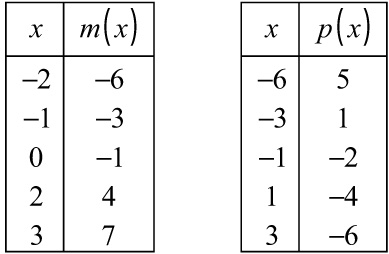
Solution: Remember to work from the inside out when composing two functions. In other words, begin with the function that’s plugged into the other function. In this case, you begin by calculating p(3). According to the p(x) table, p(3) = –6.

Now you know that m^–1(p(3)) = m^–1(–6). However, you are only given a table for m(x), not for its inverse. Remember that an inverse function simply reverses the x- and y-coordinates of a function—the inputs become outputs and vice versa. Therefore, by reversing the columns of the m(x) table, you can create a table of values for its inverse function.

According to this new table, m^–1(–6) = –2. Therefore, you conclude that m^–1(p(3)) = –2.

Parametric Equations

With all this talk about functions, you might be leery of nonfunctions. Don’t get all closed-minded on me. You can use something called parametric equations to express graphs, too, and they have the unique ability to represent nonfunctions (like circles) very easily. Parametric equations are pairs of equations, usually in the form of “x =” and “y =,” that define points of the graph in terms of yet another variable, usually t.

x = t + 1
y = t – 2

These two equations together produce one graph. To find that graph, you have to substitute a spectrum of things for the parameter t; each time you make a t substitution, you’ll get a point on the graph. So a parameter is just a variable into which you plug numeric values to find coordinates on a parametric equation graph. For example, if you plug t = 1 into the equations, you get the following:

x = t + 1 = 1 + 1 = 2
y = t – 2 = 1 – 2 = –1

Therefore, the point (2,–1) is on the graph. To get another point, I’ll plug in t = –2, but you can actually plug in any real number for t:

x = –2 + 1 = –1
y = –2 – 2 = –4

A second point on the graph is (–1,–4). You can see that this process takes a while. In fact, it seems like only an infinite number of t-values will get you the exact graph.

Converting to Rectangular Form

Let’s be honest, no one wants to plug in an infinite number of points. Even if you had the time to do that, you could definitely find something better to do. Therefore, it behooves us to learn how to translate from parametric form to the form we know and love, rectangular form. In the next example, we’ll translate that set of parametric equations into something more manageable.

Example 9: Translate the parametric equations x = t + 1, y = t – 2 into rectangular form.

Solution: Begin by solving one of the equations for t. They’re both pretty basic, so it doesn’t matter which you choose. I’ll pick the x equation so my result is in the form “y =.” That makes it easier to graph:

Now you have t in terms of x. Therefore, you can replace the t in the y equation with (x – 1), because you know that t = x – 1:

This is just a line in slope-intercept form, so your parametric equations’ graph is the line with slope 1 and y-intercept –3. It’s graphed in Figure 3.11.

Figure 3.11

The graph of y = x – 3. Note that the points (2,–1) and (–1,–4) are both on the graph, as we suspected from our work preceding Example 9.

The Least You Need to Know

• A relation becomes a function when each of its inputs can only result in one matching output.
• The inputs of a function comprise the domain and the outputs make the range.
• When a function is plugged into its inverse function (and vice versa), they cancel each other out.
• Parametric equations are defined by “x =” and “y =” equations that contain a parameter, usually t.