CHAPTER
5

Take It to the Limit

In This Chapter

• Understanding what a limit is
• Why limits are needed
• Approximating limits
• One-sided and general limits

When most people look back on calculus after completing it, they wonder why they had to learn limits at all. For some, it’s like getting all of their teeth pulled just for the fun of it. After a brief limit discussion at the start of the course, there are very few times that limits return, and when they do, it is only for a brief cameo role in the topic at hand. However, limits are extremely important in the development of calculus and in all of the major calculus techniques, including differentiation, integration, and infinite series.

As I discussed in Chapter 1, limits were the key ingredient in the discovery of calculus. They allow you to do things that ordinary math gets cranky about. In practice, limits are many students’ first encounter with a slightly philosophical math topic, answering questions like, “Even though this function is undefined at this x-value, what height did it intend to reach?” This chapter will give you a great intuitive feel of what a limit is and what it means for a function to have a limit; the next chapter will help you evaluate limits.

One final note: the official limit definition is called the delta-epsilon definition of limits. It is very complex, and is based on high-level mathematics. A discussion of this rigorous mathematical concept is not beneficial, so it is omitted here. In essence, it is possible to be a great driver without having to understand every principle of the combustion engine.

What Is a Limit?

When I first took calculus in high school, I was hip-deep in evaluating limits via tons of different techniques before I realized that I had no idea what I was doing, or why. I am one of those people who needs some sort of universal understanding in a math class, some sort of framework to visualize why I am undertaking the process at hand. Unfortunately, calculus teachers are notorious for explaining how to complete a problem (outlining the steps and rules) but not explaining what the problem means. So for your benefit and mine, we’ll discuss what a limit actually is before we get too nutty with the math part of things.

Let’s start with a simple function: f(x) = 2x + 5. You know that this is a line with slope 2 and y-intercept 5. If you plug x = 3 into the function, the output will be f(3) = 2(3) + 5 = 11. Very simple, everyone understands, everyone’s happy. What else does this mean, however? It means that the point (3,11) belongs to the relation and function I call f. Furthermore, it means that the point (3,11) falls on the graph of f(x), as evidenced in Figure 5.1.

Figure 5.1

The point (3,11) falls on the graph of f(x).

All of this seems pretty obvious, but let’s change the way we talk just a little to prepare for limits. Notice that as you get closer and closer to x = 3, the height of the graph gets closer and closer to y = 11. In fact, if you plug x = 2.9 into f(x), you get f(2.9) = 2(2.9) + 5 = 10.8. If you plug in x = 2.95, the output is 10.9. Inputs close to 3 give outputs close to 11, and the closer the input is to 3, the closer the output is to 11.

Even if you didn’t know that f(3) = 11 (say for some reason you were forbidden by your evil stepmother, as was Cinderella), you could still figure out what it would probably be by plugging in an insanely close number like 2.99999. I’ll save you the grunt work and tell you that f(2.99999) = 10.99998. It’s pretty obvious that f is headed straight for the point (3,11), and that’s what is meant by a limit.

A limit is the intended height of a function at a given value of x, whether or not the function actually reaches that height at the given x. In the case of f, you know that f does reach the value of 11 when x = 3, but that doesn’t have to be the case for a limit to exist. Remember that a limit is the height a function intends to reach.

Can Something Be Nothing?

You may ask, “How am I supposed to know what a function intends to do? I don’t even know what I intend to do.” Luckily, functions are a little more predictable than people, but more on that later. For now, let’s look at a slightly harder problem involving limits. But before we do, let’s discuss how a limit is written in calculus.

In our previous example, we determined that the limit, as x approaches 3, of f(x) equals 11, because the function approached a height of 11 as we plugged in x values closer and closer to 3. As it seems with everything else, calculus has a shorthand notation for this:

This is read, “The limit, as x approaches 3, of f(x) equals 11.” The tiny 3 is the number you’re approaching, f(x) is the function in question, and 11 is the intended height of f at 3. Now, let’s look at a slightly more involved example.

Figure 5.2 is the graph of . Clearly, the domain of g cannot contain x = –2, because that causes 0 in the denominator, and that is just plain yucky.

Notice that the graph of g has a hole at the evil value of x = –2, but that won’t stop us. We’re going to evaluate the limit there. Remember, the function doesn’t actually have to exist at a certain point for a limit to exist—the function only has to have a clear height it intends to reach. Clearly, the function has an intended height it wishes to reach when x = –2 in the graph—there’s a gaping hole at that exact spot, in fact.

Figure 5.2

The graph of .

How can you evaluate ? Just as we did in the previous example, you’ll plug in a number insanely close to x = –2, in this case, x = –1.99999. Again, I’ll do the grunt work for you (you can thank me later): g(–1.99999) = –4.99999. Even a knucklehead like me can see that this function intends to go to a height of –5 on the function g when x = –2.

Therefore, , even though the point (–2,–5) does not appear on the graph of g(x). This is one example of a limit existing because a function intends to go to a height despite not actually reaching that height.

Example 1: Graph and simplify the function to evaluate .

Solution: You might be thinking, “Graph something that complicated? How am I supposed to do that?” While you could spend an hour plotting points on the graph by substituting x-values into the function, there’s no need. Like the function g(x) graphed in Figure 5.2, f(x) will have a much simpler graph than you may initially think.

Begin by factoring the numerator of

Notice that the common factor (x – 4) appears in the numerator and denominator of the fraction. You can simplify the fraction by eliminating the common factor, basically crossing out (x – 4) like so:

This means the values of are exactly the same as the values of f(x) = 2x – 1, with one gigantic exception. The original version of the function is a fraction, and if you substitute x = 4 into it, you get 0 in the denominator, which is not allowed.

What does all that mean? The graphs of and f(x) = 2x – 1 look exactly the same except when x = 4. At that point on the line, you should place a hole in the graph, as illustrated in Figure 5.3.

Figure 5.3

The graph of , which is not defined when x = 4. Note that it matches the graph of y = 2x – 1, except at x = 4.

Now to calculate . Even though f(x) is not defined when x = 4, y = 2x – 1 is, and we know that the graphs exactly match each other everywhere else. Therefore, intends to reach the height f(x) = 2x – 1 reaches when x = 4. To calculate that height, substitute x = 4 into the simplified version of f(x).

You conclude that , which you can verify visually using the graph in Figure 5.3.

One-Sided Limits

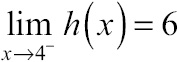
Occasionally, a function will intend to reach two different heights at a given x, one height as you come from the left side and one height as you come from the right side. We can still describe these one-sided intended heights, using left-hand and right-hand limits. To better understand this bizarre function behavior, look at the graph of h(x) in Figure 5.4.

Figure 5.4

The graph of h(x) consists of two pieces; a graph like this is usually the result of a piecewise-defined function.

This graph does something very wacky at x = 4: it breaks. Trace your finger along the graph as it approaches x = 4 from the left. What height is your finger approaching as you get close to (but don’t necessarily reach) x = 4? You are approaching a height of 6. This is called the left-hand limit and is written like this:

The little negative sign in the exponent indicates that you should only be interested in the height the graph approaches as you travel along the graph from the left-hand side. If you trace your finger along the other portion of the graph, this time toward x = 4 from the right, you’ll notice that you approach a height of 2 when you get close to x = 4. This is, as you may have guessed, the right-hand limit for x = 4, and it is written as follows:

Example 2: Graph the function k(x), defined here. Then, evaluate (a) and (b) .

Solution: If you need to review piecewise-defined functions, check out Example 2 in Chapter 3.

The function k(x) is defined by two linear equations. Its values come from y = –x – 3 whenever –1 > x ≥ 1. It may help you to split that compound inequality into two simple inequalities: –1 > x and x ≥ 1. (It also may help to rewrite –1 > x with x on the left side: x < –1.) Basically, values of k(x) are generated by the expression –x – 3 for x-values less than –1 or greater than or equal to 1.

Similarly, values of k(x) are generated by the expression 2x + 2 for x-values greater than or equal to –1 and less than 1. (Break the compound inequality into two simple inequalities again if that helps you visualize the interval.) The graph of k(x) appears in Figure 5.5.

Figure 5.5

The graph of k(x) and four points of interest, the endpoints of the linear segments that form k(x).

Although your graph may be slightly inaccurate if you mix up the open and solid dots on your graph, it won’t affect the limit values at x = –1 and x = 1. Speaking of the limit values, it’s time to get calculating.

To evaluate , you need to identify the height that k(x) intends to reach as you approach x = –1 from the left. Trace your finger from left to right along the graph, beginning at its left edge and approaching x = –1. Stop at x = –1, right before the graph jumps from point (–1,–2) to (–1,0). As you approach x = –1 from the left, the function intends to reach point (–1,–2), with an intended height of –2. Therefore, .

Figure 5.6

Calculating the left- and right-hand limits of k(x) as x approaches –1.

To calculate , approach that same break in the graph at x = –1, but this time approach from the right side, tracing your finger along y = 2x + 2 as it declines steeply. (Remember, you’re approaching x = –1 from right to left.) Again, stop before the jump in the graph at x = –1, this time at the point (–1,0). This line has an intended function height of 0, so .

Until now, we have only spoken of a general limit (in other words, a limit that doesn’t involve a direction, such as from the right or left). Most of the time in calculus, you will worry about general limits, but in order for general limits to exist, right- and left-hand limits must also be present; this we learn in the next section, which will tie together everything we’ve discussed so far about limits. Can you feel the electricity in the air?

When Does a Limit Exist?

If you don’t understand anything else in this chapter, make sure to understand this section. It contains the two essential characteristics of limits: when they exist and when they don’t. If you’ve understood everything so far, you’re on the verge of understanding your first major calculus topic. I’m so proud of you—I remember when you were only this tall.

Here’s the key to limits: in order for a limit to exist on a function f at some x-value (we’ll give it a generic name like x = c), three things must happen:

1. The left-hand limit must exist at x = c.

2. The right-hand limit must exist at x = c.

3. The left- and right-hand limits at c must be equal.

In calculus books, this is usually written like this: if exists and is equal to the one-sided limits.

The diagram in Figure 5.7 will help illustrate the point.

Figure 5.7

Yet another hideous graph called f(x). Can you spot where the limit doesn’t exist?

There are two interesting x-values on this graph: x = –1 and x = 6. At one of those values, a general limit exists, and at the other, no general limit exists. Can you figure out which is which using the guidelines?

You’re reading ahead, aren’t you? Well, stop it. Don’t read any more until you’ve actually tried to answer the question I’ve asked you. Do it. I’m watching!

The answer: exists and does not. Remember, in order for a limit to exist, the left- and right-hand limits must exist at that point and be equal. As you approach x = –1 from the left and right sides, each time you are heading toward a height of 5, so the two one-sided limits exist and are equal, and we can conclude that (i.e., the general limit as x approaches –1 on f(x) is equal to 5).

However, this is not the case when we approach x = 6 from the right and left. In fact, , whereas . Because those one-sided limits are unequal, we say that no general limit exists at x = 6, and that does not exist.

Visually, a limit exists if the graph does not break at that point. For the graph f(x) in question, a break occurs at x = 6 but not x = –1, which means a limit doesn’t exist at the break but can exist at the hole in the graph. Remember that a limit can exist even if the function doesn’t exist there—as long as the function intends to reach the same height from the left and the right, the limit exists.

• A general limit does not exist if the left- and right-hand limits aren’t equal.

In other words, if there is a break in the graph of a function, and the two pieces of the function don’t meet at an intended height, then no general limit exists there. In Figure 5.8, does not exist because the left- and right-hand limits are unequal.

Figure 5.8

The graph of g(x).

• A general limit does not exist if a function increases or decreases infinitely at a given x-value (i.e., the function increases or decreases without bound).

In order for a general limit to exist, the function must approach some fixed numerical height. If a function increases or decreases infinitely, then no limit exists. In Figure 5.9, does not exist because h(x) has a vertical asymptote at x = c, causing the function to increase without bound there. A limit must be a finite number in order to truly exist.

Figure 5.9

The graph of h(x).

• A general limit does not exist if a function oscillates infinitely, never approaching a single height.

This is rare, but sometimes a function will continually wiggle back and forth, never reaching a single numeric value. If this is the case, then no general limit exists. Because this is so rare, most calculus books give the same example when discussing this eventuality, and I will be no different. (Math peer pressure is harsh, let me tell you.) No general limit exists at x = 0 in Figure 5.10 because the function never settles on any one value the closer you get to x = 0.

Figure 5.10

The graph of does not exist.

Example 3: A function f(x) is defined by the graph in Figure 5.11. Based on the graph and your amazing knowledge of limits, evaluate the limits that follow. If no limit exists, explain why.

Figure 5.11

The hypnotic graph of f(x). Mortal men may turn to stone upon encountering its terrible visage.

(a)

Solution: As you approach x = –4 from the right, the function increases without bound. You have two ways to write your answer; either say that the limit does not exist because the function increases infinitely, or write .

(b)

Solution: As you approach x = 4 from the right and left, the function approaches a height of 3. Therefore, the general limit exists and is 3.

(c)

Solution: No general limit exists here because the left-hand limit (1) does not equal the right-hand limit (–3).