CHAPTER
15

Antiderivatives

In This Chapter

• “Un-deriving” expressions
• The Power Rule for Integration
• Integrating trigonometric functions
• Don’t hate, separate!
• The Fundamental Theorem: the connection to area
• The key to u-substitution

Are you a little perplexed? Probably. We spent the first 13 chapters of the book discussing complex mathematical procedures, and then suddenly and without warning we’re calculating the area of rectangles in Chapter 14. Kind of a letdown, I know. Most people have this terrifying view of calculus, and assume that everything in it is impossible to understand; they are usually surprised to be calculating simple areas this deep in the course.

In this chapter, we’ll find exact areas beneath a curve. We’ll also uncover one of the most fascinating mathematical relationships of all time: the area beneath a curve is related to the curve’s antiderivative. You heard me right— antiderivative. After all this time learning how to find the derivative of a function, now we’re going to go backward and find the antiderivative. Before, we took f(x) = x³ – 2x² and got f ′(x) = 3x² – 4x; now, we’re going to start with the derivative and figure out the original function.

It’s a whole new ballgame, and we’re going to learn everything from the first half of the course in reverse. For those of us who always seem to do things backwards, this should come as a welcome change! Sound exciting? Sound painful? It’s a little from column A and a little from column B.

The Power Rule for Integration

Before we get started, let’s talk briefly about what reverse differentiating means. The process of going from the expression f ′(x) back to f(x) is called antidifferentiation or integration—both words mean the same thing. The result of the process is called an antiderivative or an integral. Basically, an antiderivative (or integral) is the opposite of a derivative.

Integration is denoted using a long, stretched-out letter S, like this:

This is read “The integral of 2x, with respect to x, is equal to x² plus some unknown constant” (called the constant of integration). This integral expression is called an indefinite integral because there are no boundaries on it.

Why do you have to use a constant of integration? Lots of functions have the same derivative—for example, both h(x) = x³ + 6 and j(x) = x³ – 12 have the same derivative, 3x². Therefore, when we integrate , you say the antiderivative is x³ + C, because you have no way of knowing what constant was in the original function.

Whereas an indefinite integral has no boundaries next to the integration sign, a definite integral does. For example, is a definite integral because it contains the limits of integration 1 and 3. The result of an indefinite integral is a new expression, but the result of a definite integral is a real number. For example, , but . (You’ll learn how to solve these kinds of problems soon.)

Both definite and indefinite integrals contain a “dx”; don’t worry about this little piece—you don’t have to do anything with it. Just make sure its variable matches the variable in the function (in this case, x).

That’s a lot of vocabulary for now. Before you get overwhelmed, let’s get into the meat of the mathematics. Remember finding simple derivatives with the Power Rule? There’s a way to find simple integrals using the Power Rule for Integration. Instead of multiplying the original coefficient by the exponent and then subtracting 1 from the power, you’ll add 1 to the power and divide by the new power.

The Power Rule for Integration: The integral of a single variable to some power is found by adding 1 to the existing exponent and dividing the variable by the new exponent:

Remember, you can only use the Power Rule for Integration if you are integrating a single variable to a power, just like the regular Power Rule. However, if the only thing standing in your way is a coefficient, you are allowed to yank it out of the integral to get it out of your way, as indicated in the first example.

Example 1: Evaluate .

Solution: Even though there are two terms here, each is simply a variable to some power with a coefficient attached. You can actually separate addition or subtraction problems into separate integrals as follows:

Don’t worry about the or dx in the problem. They’re the “bookends” of an integral expression, marking where it begins and ends; just integrate whatever falls between them. Before you can apply the Power Rule for Integration, you should “pull out” the coefficients:

Now the expression in each integral looks like the one in the Power Rule for Integration theorem. Add 1 to each power and divide each variable by its new power. The integral sign and the “dx” will disappear, but don’t forget to add “+ C” to the end of the problem, because all indefinite integrals require it:

Integrating Trigonometric Functions

As with learning trigonometric derivatives, learning trigonometric integrals just means memorizing the correct formulas. If you forget them, you can actually create some of them from scratch easily (like the integral of the tangent function, as you’ll see later in the chapter). However, not all of them are quite so easy to build by yourself, so I see some quality memorizing time in your not-too-distant future.

I can tell by that unhappy look on your face that the thought of more memorizing doesn’t excite you. (You’re going to be even unhappier if you haven’t flipped ahead to the actual formulas yet—they are crazy looking.) Think back. You had to memorize the multiplication tables in elementary school, remember? This is just sort of the grandfather of the multiplication tables, but important all the same.

And now, with no further ado, here are the trigonometric functions with their antiderivatives:

           

There are a lot of natural log functions in the list of trig integrals. That is due, in no small part, to the fact that , another important formula to memorize.

Here’s another, while we’re at it: the integral of e^x is itself, just like it was its own derivative; therefore, . Integrating logarithmic functions is very, very tricky, so we don’t even attempt that in Calculus I. We’ll save that for Calculus II—that way you have something to look forward to! (Or dread. Take your pick.)

Example 2: Integrate: .

Solution: Rewrite this sum as a sum of two separate integrals:

The radical can be expressed as a fractional exponent , which means you can apply the Power Rule for Integration:

To complete the problem, recall that .

While technically both integrals produce a coefficient of integration (C), you can add those constants to a new (and still completely unknown) constant C. Is it weird to add C to C and get C? Yes, but remember that we have no idea what C equals, and we have no way of ever finding out in the context of indefinite integrals. For all intents and purposes, just remember to staple a single “+ C” to the end of any indefinite integral, no matter how many individual integrals you introduce along the way.

Separation

Breaking up is hard to do, but under specific circumstances, it is really quite worthwhile. Sometimes things just don’t work out, and fractions have to go their separate ways. After a long, sunny time in the numerator together, terms just want a little more “me” time and some personal space. However, after all the time they’ve spent together, they’ve saved up a little bundle in the denominator, and both want to walk away with it.

The good news is, in the math world, both pieces of the numerator get a full share of the denominator—no lawyers, no haggling over how it should be broken up. Both terms of the numerator walk away with a full denominator, and are a little wiser for having gotten involved in the first place.

Back in grade school, you learned that two fractions couldn’t be added unless they had the same denominator. With this knowledge, you proudly calculated things like and never looked back. Well, look at it backward for just a moment. If you are given the fraction , you can rewrite it as , just as you know that .

Top-heavy integrals (which have lots of terms in the numerator but only one in the denominator) and other fractional integrals are occasionally easier to solve if you split the larger integral into smaller, more manageable ones. Although the original problem couldn’t be solved via u-substitution or the Power Rule, the smaller integrals usually can.

Example 3: Find using the separation technique.

Solution: This is a fraction, so the Power Rule for Integration doesn’t apply, and setting the numerator or denominator equal to u is not going to do a whole lot for you, so u-substitution is out. If, however, you separate the five terms of the large numerator into five separate fractions, watch what happens:

When you simplify each of these fractions, you get simple integrals, each of which can be integrated via the Power Rule for Integration:

The Fundamental Theorem of Calculus

Finally, it’s time to solve two mysteries of recent origin: how do you find exact areas under curves, and why are we even mentioning areas—isn’t this chapter about integrals? It turns out that the exact area beneath a curve can be computed using a definite integral. This is one of two major conclusions, which together make up the Fundamental Theorem.

Part One: Areas and Integrals Are Related

After all the time we spent approximating it in Chapter 14, we’re finally going to calculate the exact area beneath y = x² + 1 on the interval [0,3].

From now on, we’re going to equate definite integrals with the area beneath a curve (technically speaking, the area between the function and the x-axis, remember?). Therefore, I can say that the area beneath x² + 1 on the interval [0,3] is equal to .

This new notation is read, “the integral of x² + 1, with respect to x, from 0 to 3.” Unlike indefinite integrals, the solution to a definite integral, such as this one, is a number. That number is, in fact, the area beneath the curve. How in the world do you get that number, you ask? How about a warm welcome for the Fundamental Theorem?

The Fundamental Theorem of Calculus (part one): If g(x) is the antiderivative of the continuous function f(x), then .

In other words, to calculate the area beneath the curve f(x) on the interval [a,b], you must first integrate the function. Then, plug the upper bound (b) into the integral. From this value, subtract the result you get from plugging the lower bound (a) into the same integral. It’s a brilliantly simple process, as powerful as it is elegant.

Example 4: Once and for all, find the exact area beneath the curve f(x) = x² + 1 on the interval [0,3] using the Fundamental Theorem of Calculus.

Solution: This problem asks you to evaluate the definite integral:

Begin by integrating x² + 1 using the Power Rule for Integration. When you complete the integral, you no longer write the integration symbol, and you do not write “+ C.” Instead, draw a vertical slash to the right of the integral, and copy the limits of integration onto it. This signifies that the integration portion of the problem is done:

Plug 3 into the function (for both x’s) and subtract 0 plugged into the function:

Part Two: Derivatives and Integrals Are Opposites

I kind of spoiled this revelation for you already—I’m sorry. However, the second major conclusion of the Fundamental Theorem still holds some surprises. Let’s check out the theorem first:

The Fundamental Theorem of Calculus (part two): If f(x) is a continuous and differentiable function, , if a is a real number.

That looks unsightly. Here’s what it means without all the gobbledygook. Let’s say you’re taking the derivative of a definite integral whose lower bound is a constant (i.e., just a number) and whose upper bound contains a variable. If you take the derivative of the entire integral with respect to the variable in the upper bound, the answer will be the function inside the integral sign (unintegrated), with the upper bound plugged in, multiplied by the derivative of the upper bound. This theorem looks, feels, and even smells complex, but it’s not hard at all. Trust me on this one. All you have to do is learn the pattern.

Example 5: Evaluate .

Solution: You don’t have to use the shortcut in part two of the Fundamental Theorem, but it makes things easier. Notice that the variable expression is in the lower (not the upper) bound, which is not allowed by the theorem. Therefore, you should swap them using a property of integrals I discussed earlier in the chapter. It says that flip-flopping the boundaries of an integral is fine, as long as you multiply the integral by –1.

Because you are deriving with respect to x (and x is in the upper bound) and the lower bound is a constant, you are clear to apply the new theorem. All you do is plug the upper bound (sin x) into the function t² to get (sin x)², and multiply by the derivative of the upper bound (which will be cos x). Don’t forget the negative, which stays out in front of everything:

–sin² x ∙ cos x

Here’s a question for you: what if you forget this theorem? No problem—you can do Example 5 the long way, working from the inside out. Start with the integration problem and then take the derivative. You’ll get the same thing. If you apply the Fundamental Theorem (part one) to the integral, you get:

Take the derivative with respect to x to get –sin² x ∙ cos x. Don’t forget to apply the Chain Rule when differentiating ; that’s where cos x comes from.

You don’t always have to switch the boundaries and make the integral negative. Only do it if the constant appears in the upper boundary. What happens if both boundaries contain variables? If this is the case, you can’t use the shortcut offered by the theorem and must resort to the long way.

u-Substitution

At this point, you can’t solve too many integration problems. You should have a handful of antiderivatives memorized (such as and ) and should have a pretty good grip on the Power Rule for Integration (meaning, for instance, you know that ). However, what do you do if both of those techniques fail? You look, with hope glinting in your eyes, to a new method—u-substitution. You’ll use u-substitution almost as much as the Power Rule for Integration—it’s a calculus heavy hitter.

The key to u-substitution is finding a piece of the function whose derivative is also in the function. The derivative is allowed to be off by a coefficient, but otherwise must appear in the function itself.

Here are the steps you’ll follow when u-substituting:

1. Look for a piece of the function whose derivative is also in the function. If you’re not sure what to use, try the denominator or something being raised to a power in the function.

2. Set u equal to that piece of the function and take the derivative with respect to x.

3. Use your u and du expressions to replace parts of the original integral, and your new integral will be much easier to solve.

Example 6: Use u-substitution to find (i.e., prove that the integral of tangent is equal to ).

Solution: Set u equal to a piece of the integral whose derivative is also in the integral. Because sine and cosine are both present (and the derivative of each is basically the other function), you could pick either one to be u, but remember the hint I gave you: if you’re not sure which expression to choose, pick the denominator or something to a power. Therefore, set u = cos x and derive with respect to x to get du = –sin x dx.

There’s the sin x you expected. It, like u = cos x, appears in the integral. Well, almost. In the original integral, sin x is positive, so multiply both sides of du = –sin x dx by –1 so that the sine functions match:

–du = sin x dx

Now it’s time to write the original integral with u’s instead of x’s. Instead of sin x, the new numerator is –du (because –du = sin x dx). The new denominator is u (because u = cos x).

Remember that the integral of , so . The final step is to replace the u using your original u equation (u = cos x) to get the final answer of .

The trickiest part of u-substitution is deciding what u should be. If your first choice doesn’t work, don’t sweat it. Try something else until it works out for you. It eventually will. The only way to get really good at this is to practice, practice, practice. Eventually, picking the correct u will become easier.

Tricky u-Substitution and Long Division

When we first discussed u-substitution, I made it a point to say that the derivative of u must appear in the problem. This is usually true, so I wasn’t technically lying. There is a way to use u-substitution, even if it’s not the most obvious choice.

Example 7: Find .

Solution: For grins, let’s go ahead and try to find the antiderivative using u-substitution. Once again, remember our tip: if you’re not sure what to set equal to u, try the denominator. Therefore, u = x – 2 and du = dx. If you make the appropriate substitutions back into the problem, you get:

To be honest, it doesn’t look much better than the original, does it? Don’t give up, though; we’re not out of options. Go back to your u equation and solve it for x to get:

Now substitute that x value into the numerator of our integral, and suddenly everything is a little cheerier:

At least all of our variables are the same now. That’s a relief. Can you see where to go from here? This fraction is top-heavy, with lots of terms in the numerator but only one in the denominator, so we can use the separation method from last section to finish. What a happy coincidence that we just learned it!

You may be wondering why the – 4 vanished in the last step. Remember that C is some constant you don’t know. If you subtract 4 from that, you’ll get some other number (which is 4 less than the original mystery number). Since I still don’t know the value for C, I just write it as C again, instead of writing C – 4.

There are alternatives when integrating fractions like these. In fact, you can begin a rational integral by applying long division; it helps to simplify the problem if the numerator’s degree is greater than or equal to the denominator’s degree. It works like a charm if the denominator is not a single term, as is the case with this example.

Because the degree of the numerator (1) is greater than or equal to the degree of the denominator (1), begin by dividing 2x – 1 by x – 2:

Therefore, you can rewrite the integral as , and tricky u-substitution is no longer required. The solution will again be .

Technology Focus: Definite and Indefinite Integrals

Symbolic calculators like the TI-89 are very powerful integration machines. They work whether you’re dealing with indefinite integrals (which have no bounds of integration) or definite integrals (which do).

In Example 1 from this chapter, you applied the Power Rule for Integration to determine that . To check the answer with your TI-89, you need to access the calculus tools in the f 3 menu. Integration is option 2, as illustrated in Figure 15.1.

Figure 15.1

The integration tool is located just beneath the differentiate tool you used in Chapter 9.

As with differentiation, you follow the expression by a comma and then the variable that comes after the “d” in the problem. For example, this problem contains “dx” so you should type “,X” before you close the expression with a parenthesis (see Figure 15.2).

Figure 15.2

The solution verifies our solution to Example 1.

The calculator’s solution looks a little different from our solution. For one thing, it lists the terms in order of exponent, from greatest to least. It also does not list the required “+ C” as part of the solution. Remembering that constant is up to you.

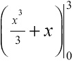
To compute a definite integral on your TI-89, enter the lower and upper bounds immediately following “,X” and separate them with commas. For example, in Example 4 you concluded that . Check this answer by entering the expression in Figure 15.3.

Figure 15.3

If you’re faced with a definite integral, be sure to include the bounds.

Are you ready to be really impressed with a symbolic calculator? You can use them to check problems like Example 5, which are Fundamental Theorem of Calculus problems containing multiple variables (see Figure 15.4).

Figure 15.4

The TI-89 correctly computes the derivative, with respect to x, of a definite integral written in terms of t that has a lower bound defined as a function of x!

For those of you not wielding the humbling power of a symbolic calculator, hope is not lost. Your TI-84 may not be able to figure out definite integrals, but definite integrals are a snap. Press the button and scroll down to “9:fnInt(” as illustrated in Figure 15.5.

Figure 15.5

You can’t spell “fnInt” without “fun”! Never mind—you absolutely can.

If you have MathPrint enabled on your calculator, you are greeted with a fancy template into which you can plug your definite integral (see Figure 15.6).

Figure 15.6

Insert your bounds, the expression you’re integrating, and the variable you’re integrating with respect to into the appropriate boxes.

When you do, you get the correct answer of 12, as illustrated in Figure 15.7.

Figure 15.7

The right solution is definitely 12. Hooray for disappointing math puns!

If MathPrint is not enabled, you enter the expression exactly as you would on the TI-89 (see Figure 15.8).

Figure 15.8

If you don’t want to be bothered with arrowing between the boxes in the MathPrint template, you can compute the definite integral by typing this command.

The Least You Need to Know

• Integration, like differentiation, has a Power Rule of its own, in which you add 1 to the exponent and divide by the new exponent.
• Trigonometric functions have bizarre integrals, some of which are difficult to produce on your own; therefore, it’s best to memorize them.
• The separation technique allows you to write an integral that’s a sum or difference as a sum or difference of separate integrals.
• The two parts of the Fundamental Theorem of Calculus tell you how to evaluate a definite integral and give a shortcut for finding specific derivatives of integral expressions.
• u-substitution helps you integrate expressions that contain functions and their derivatives.
• Long division and tricky u-substitution are useful tools in your integration repertoire.