CHAPTER
10

Common Differentiation Tasks

In This Chapter

• Equations of tangent and normal lines
• Differentiating equations containing multiple variables
• Derivatives of inverse functions
• Differentiating parametric equations
• Solving gross equations with your calculator

Even though the derivative is just the slope of a tangent line, its uses are innumerable. We’ve already seen that it describes the instantaneous rate of change of a nonlinear function. However, that hardly explains why it’s one of the most revolutionary mathematical concepts in history. Soon we’ll be exploring more (and substantially more exciting) uses for the derivative.

In the meantime, there’s a little bit more grunt work to be done. (That makes you happy to read, doesn’t it?) This chapter will help you perform specific tasks and find derivatives for very particular situations. Think of learning derivatives as being like trying to get your body in shape. In the last chapter, you learned the basics, the equivalent of a good cardiovascular workout, working all of your muscles in harmony with each other. In this chapter, we’re working out specific muscle groups, one section at a time. There’s not a lot of similarity between each individual topic here, but exercising all of these abilities at the appropriate time (and knowing when that time arrives) is essential to getting yourself in shape mathematically.

Finding Equations of Tangent Lines

Writing tangent line equations is one of the most basic and foundational skills in calculus. You already know how to create the equation of a line using point-slope form (see Chapter 2). Since it’s the equation of a tangent line you’re after, the slope is the derivative of the function! All that’s left to do is figure out the appropriate point, and if that were any easier, it’d be illegal.

Example 1: Write the equation of the tangent line to the curve f(x) = 3x² – 4x + 1 when x = 2.

Solution: Take a look at the graph of f(x) in Figure 10.1 to get a sense of our task.

Figure 10.1

The graph of f(x) = 3x² – 4x + 1 and a future point of tangency.

You want to find the equation of the tangent line to the graph at the indicated point (when x = 2). This is the point of tangency, where the tangent line will strike the graph. Therefore, this point is both on the curve and on the tangent line. Since point-slope form requires you to know a point on the line in order to create the equation of that line, you’ll need to know the coordinates of this point. Since you already know the x value, plug it into f(x) to get the corresponding y value:

So the point (2,5) is on the tangent line. Now all you need is the slope of the tangent line, f ′ (2):

Now that you know a point on the tangent line and the correct slope, slap those values into point-slope form and out pops the correct tangent line equation:

Figure 10.2 verifies the solution visually.

Figure 10.2

The (dotted) line y = 8x – 11 is tangent to f(x) at x = 2.

Occasionally you’ll be asked to find the equation of the normal line to a curve. Because the normal line is perpendicular to the tangent line at the point of tangency, you use the same point to create the normal line, but the slope of the normal line is the negative reciprocal of the slope of the tangent line.

Example 2: Calculate the slope of the normal line to the curve g(x) = tan (x² – π) at , reporting the answer accurate to the thousandths place.

Solution: Now this is a crazy-looking graph. I definitely do not recommend trying to sketch it by hand. If you don’t mind spoilers, go ahead and peek at Figure 10.3. Anyway, enough gawking. Let’s keep moving. Remember, the slope of the normal line is perpendicular to the slope of the tangent line. Apply the Chain Rule to calculate the derivative of g(x):

Now calculate . It is going to get messy, so plan on using decimal forms provided by your calculator.

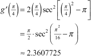
Although that number was a little ugly looking, you’re headed in the right direction. This is the perfect time to double-check your derivative with your calculator, as demonstrated in Figure 10.3.

Figure 10.3

If decimals bring you no joy, I’d argue that knowing the actual value of the derivative, 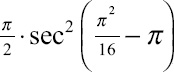, isn’t much better.

The slope, m, of the normal line to g(x) at is the opposite reciprocal of the slope of the tangent line:

In this section, we’ll take the derivative of equations containing x and y, and I will always ask you to find the derivative with respect to x. What is the derivative of y with respect to x, you ask? The answer is this notation: . It is literally read, “the derivative of y with respect to x.” The numerator tells you what you’re deriving, and the denominator tells you what you’re respecting.

Let’s try a slightly more complex derivative. What is the derivative of 3y², with respect to x? The first thing to notice is that the variable in the expression does not match the variable you’re respecting, so you treat the y as a completely separate function and apply the Chain Rule. I know you’re not used to using the Chain Rule when there’s only a single variable inside the function, but if that variable is not the variable you’re respecting, you have to give it a hard time and “rough it up” a little. So to differentiate 3y², start by deriving the outer function and leaving y (the inner function) alone to get 6y. Now multiply this by the derivative of y with respect to x, and you get:

You will encounter odd derivatives like this whenever you cannot solve an equation for y or for f(x). You may not have noticed, but every single derivative question until now has been worded “Find the derivative of y = …” or “Find the derivative of f(x) ….” When a problem asks you to find in an equation that cannot be solved for y, you have to resort to the process of implicit differentiation, which involves deriving variables with respect to other variables. Whereas in past problems the derivative would be indicated by y’ or f ′(x), the derivative in implicit differentiation is indicated by .

Example 3: Find the slope of the tangent line to the graph of x² + 3xy – 2y² = –4 at the point (1,–1).

Solution: Yuck! Clearly this is not solved for y, and if you try to solve for y, you’ll get discouraged quickly—solving it for y is impossible due to that blasted y². Implicit differentiation to the rescue! The first order of business is finding the derivative of each term of the equation with respect to x. Because you’re new at this, I’ll go term by term.

The derivative of x² with respect to x is 2x. Nothing fancy is needed, since the variable in the term is the variable we’re respecting. However, in the next term, 3xy, you have to use the Product Rule, since there are two variable terms multiplied (3x and y).

Remember that the derivative of y, with respect to x, is , so the correct derivative of 3xy is . Finally, the derivative of –2y² is and the derivative of –4 is 0.

Don’t forget to differentiate on both sides of the equation! Even though I differentiate implicitly pretty often, I still sometimes forget to differentiate a constant term to get 0. I know; I’m a lunkhead.

All together now, you get a derivative of:

Move all of the terms not containing a to the right side of the equation. Once you’ve done that, factor the common out of the terms on the left side of the equation:

To finally get the derivative by itself, divide both sides of the equation by 3x – 4y:

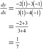
That’s the derivative. The problem asks you to evaluate it at (1,–1), so plug those values in for x and y to get your final answer:

Differentiating an Inverse Function

Let’s say you’re given the function f(x) = 7x – 5 and are asked to evaluate , the derivative of the inverse of f(x) when x = 1. To find the answer, you would first find the inverse function (using the process we reviewed in Chapter 3) and then find the derivative. However, did you know that you can evaluate the derivative of an inverse function even if you can’t find the inverse function itself? (Insert dramatic soap opera music here.) You’ll learn how to do it in just a second, but we have to review one skill first.

It’s important that you’re able to find values for an inverse function given only the original function before we try anything more difficult. The procedure we’ll use is based on one of the most important properties of inverse functions: if the point (a,b) is on the graph of f(x), then the point (b,a) is on the graph of f –1(x). In other words, if f(a) = b, then f –1(b) = a.

Example 4: If g(x) = x³ + 2, evaluate g^–1(1).

Solution:

Method 1: The easiest way to do this is to figure out exactly what g^–1(1) is and then plug in 1. According to our procedure from Chapter 3, here’s how you’d go about doing that:

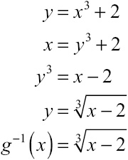
Therefore, . However, there is another way to do this without actually finding g^–1(1) first.

Method 2: You’re asked to find the output of g ^–1 (x) when its input is 1. Remember, I just said that f(a) = b implies f ^–1(b) = a, so therefore the output of g ^–1(x) when you input 1 is the same exact thing as the input of the original function g(x) when you output 1. So set the original function equal to 1 and solve; the solution will be g ^–1(1):

Either method gives you the same answer.

Now that you possess this skill, we can graduate to finding values of the derivative of a function’s inverse (say that 10 times fast, I dare you). As is the case with just about everything in calculus, there is a theorem governing this practice:

So evaluating the derivative is as simple as plugging the value into this slightly more complex, fractiony-looking formula. Once you substitute, your first objective will be to evaluate f ^–1(x) in the denominator (a skill which we just finished practicing, by no small coincidence).

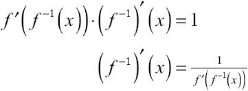
By the way, are you wondering where this formula comes from? It is pretty easy to generate. Start with the simple inverse function property f (f ^–1(x)) = x and take the derivative with the Chain Rule:

Example 5: If f(x) = x³ + 4x + 1, evaluate .

Solution: According to the formula you learned only moments ago:

Start by evaluating f ^–1(2), which is the equivalent of solving the equation x³ + 4x + 1 = 2. This is not an easy equation to solve; in fact, you can’t do it by hand. You’ll have to use some form of technology to solve the equation, whether it be a graphing calculator equation solver or a mathematical computer program.

One way to solve this equation is to set the equation equal to zero and calculate the x-intercept on a graphing calculator. See the final section of this chapter (“Technology Focus: Solving Gross Equations”) for step-by-step walkthroughs that explain how to solve equations with your graphing calculator (including this gross equation).

Whichever method you choose, the answer is x = 0.2462661722, which you can plug into the formula:

I know that’s a lot of decimals, but I didn’t want to round any of them until the final answer, or it would have compounded the inaccuracy with every step.

Parametric Derivatives

In order to find a parametric derivative, you differentiate both the x and y components separately and divide the y derivative by the x derivative. In fancy-schmancy mathematical form, it looks like this:

This formula suggests that you should derive with respect to t, but you should derive with respect to whatever parameter appears in the problem. In the following example, for instance, you’ll derive with respect to θ.

Example 6: Find the slope of the tangent line to the parametric curve defined by x = cos θ and y = 2sin θ when (pictured in Figure 10.4).

Solution: Since the parameter in these equations is θ, the derivative of the set of parametric equations is:

Calculate each derivative:

Finally, calculate the derivative when :

Multiply the numerator by the reciprocal of the denominator to simplify the complex fraction:

The second derivative (which, like all second derivatives, has the almost incomprehensible notation ) of parametric functions is not just the derivative of the first derivative. Instead, it is the derivative of the first derivative divided by the derivative of the original x term:

Technology Focus: Solving Gross Equations

Solving linear equations is a snap once you’ve had enough practice. Quadratics take a little more work, but with the handy quadratic formula in your nerdy mathematical fanny pack/tool belt, quadratic equations are harmless. However, once you run across equations raised to the third degree or higher, all bets are off. These equations follow no mortal law. It’s the Thunderdome and you’re Mad Max, but instead of cool face paint and cars, all you have is a graphing calculator and an unsharpened pencil.

In the last section of this chapter, I’ll show you how to use your graphing calculator to bring third-degree and higher equations (in other words, gross equations) to justice.

Using the Built-In Equation Solver

Both the TI-84 and TI-89 families of calculators have similar equation-solving functionality. Let’s look at both as we try to solve the equation 2x² – 19x = –35. To be fair, that’s not a completely gross equation because it’s a quadratic and because it’s actually factorable if you add 35 to both sides and set it equal to 0. The solutions are . Once we practice with this simple equation, we can set our sights on bigger and more dangerous game.

Let’s look at the TI-89 first. When you turn the calculator on or press the button, you should see something like Figure 10.5. Select the “Numeric Solver” option.

Figure 10.5

Solutions to life’s equations are a few button presses away.

Now type your equation into the solver (see Figure 10.6) and press .

Figure 10.6

The TI-89 has something the TI-84 calculators don’t have: an equal sign. You can type your equations verbatim into the solver.

You’re prompted for a guess. We know the solutions already, but pretend for a moment that we don’t. Let’s guess 1, which is close to the actual solution of . Don’t worry about the “bound” line beneath your guess—just leave that alone.

Figure 10.7

Can the calculator solve the equation? The tension in the air is palpable ….

Warning: nothing actually happens if you press enter on your guess. You have to select the “solve” option by pressing . After muttering to itself for a few moments, the calculator displays its solution, in Figure 10.8.

Figure 10.8

Oh, trusty calculator, how could we have ever doubted you?

The process works very similarly with the TI-84. Access the solver by pressing the button and scrolling to “B:Solver…” (see Figure 10.9).

Figure 10.9

The solver is a little harder to find on the TI-84.

There’s a key difference in the TI-84 solver (pun intended): the “=” key is missing, so your equation must be set equal to 0. In order to set the equation 2x² – 19x = –35 equal to 0, you need to add 35 to both sides: 2x² – 19x + 35 = 0. Type that into the solver and press (see Figure 10.10). (To change the equation once you’ve typed it in, press the “up” button.)

Figure 10.10

Remember, equations must be equal to 0 to use the TI-84 solver.

You are prompted to guess at the answer, just like the TI-89. For grins, let’s guess 9, which is close to the actual solution of x = 7 (see Figure 10.11).

Figure 10.11

There are two solutions to this equation. Your guess determines the solution provided by your calculator.

Again, don’t mess around with the bounds settings. The button doesn’t do anything, so make sure to press , which activates the “Solve” button, written in green above the key. As you might expect, the calculator deftly returns the correct answer of x = 7 (see Figure 10.12).

The Equation-Function Connection

You may be asking yourself a key question here: how am I supposed to guess a solution? Great question—glad you asked. The easiest way to generate a guess is to look at a graph of the equation. Simply set your equation equal to 0 and then type it into the screen.

Let’s turn our attention to the gross equation from Example 5: x³ + 4x + 1 = 2. Set this equation equal to 0 by subtracting 2 from both sides:

Now enter this equation into the screen, as demonstrated in Figure 10.13.

Figure 10.13

The Y variable takes the place of the 0 in the equation you set equal to 0. Why? Keep reading to find out.

The graph of the function (Figure 10.14) crosses the x-axis somewhere between x = 0 and x = 1. In other words, the equation equals 0 somewhere on the interval (0,1). Because the graph crosses the x-axis only once, you know that the original equation, x³ + 4x + 1 = 2, has only one solution.

Figure 10.14

The solution to the equation x³ + 4x + 1 = 2 is also the x-intercept of the function Y₁ = x³ + 4x – 1.

You can use the solver to calculate the solution to the equation, and 0.5 would be a terrific guess (see Figure 10.15).

Figure 10.15

Your solver should look like this just before you press the “Solve” button.

The solution is x ≈ 0.2462661722. Here’s the key connection you’ll want to remember: a solution to an equation is equal to a root of a function if you create that function by setting the equation equal to 0.

The Least You Need to Know

• To write the equation of a tangent line, use the point of tangency and the derivative at that point in conjunction with the point-slope form of a line.
• You must differentiate implicitly if an equation cannot be solved for y.
• The derivative of a function’s inverse is given by the formula .
• To calculate a parametric derivative, divide the derivative of the y equation by the derivative of the x equation.
• Solutions to equations are equivalent to roots of functions when you create those functions by setting the equations equal to O.
• You can use your calculator’s built-in solver or x-intercepts to solve gross equations.