Appendix Q. Topics from Previous Editions
Cisco changes the exams, renaming the exams on occasion, and changing the exam numbers every time Cisco changes the exam with a new blueprint. Every time Cisco changes the exams, we make new editions of the books—and we even made a new edition of the book once without a new version of the exam. And although the publisher restarts the edition number at 1 every time the exam has a major name change, this book is one of two books in a set for the CCNA R&S exam, and these are basically the eighth editions of the content in these books.
As with every new edition, the topics Cisco chooses to put in the current exam dictates the topics I choose to put in the book; however, that means some topics disappear from the mix of topics. And sometimes, I just feel the need to keep those around for that one reader in one thousand who might care. So, we decided to copy some of the old material to this DVD appendix.
This appendix holds some topics that fit this category. These topics were in some past editions, or even in drafts that did not get published in one or two cases. Regardless, the material is here in case you find it useful. But certainly do not feel like you have to read this appendix for the current exam.
The topics in this appendix are as follows:
![]() Internal processing on Cisco switches
Internal processing on Cisco switches
![]() IOS version and other reload facts
IOS version and other reload facts
![]() Secondary IP addressing
Secondary IP addressing
![]() Internal processing on Cisco routers
Internal processing on Cisco routers
![]() OSPF configuration
OSPF configuration
![]() IOS Reorders ACEs
IOS Reorders ACEs
![]() NAT Overload (PAT) on consumer routers
NAT Overload (PAT) on consumer routers
![]() Dynamic routes with OSPFv3
Dynamic routes with OSPFv3
Note
The content under the heading “Internal Processing on Cisco Switches” was most recently published for the 100-101 Exam in 2013, in Chapter 6 of the CCENT/CCNA ICND1 100-101 Official Cert Guide.
Internal Processing on Cisco Switches
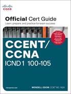
As soon as a Cisco switch decides to forward a frame, the switch can use a couple of different types of internal processing variations. Almost all of the more recently released switches use store-and-forward processing, but all three types of these internal processing methods are supported in at least one type of Cisco switch.
Some switches, and transparent bridges in general, use store-and-forward processing. With store-and-forward, the switch must receive the entire frame before forwarding the first bit of the frame. However, Cisco also offers two other internal processing methods for switches: cut-through and fragment-free. Because the destination MAC address occurs very early in the Ethernet header, a switch can make a forwarding decision long before the switch has received all the bits in the frame. The cut-through and fragment-free processing methods allow the switch to start forwarding the frame before the entire frame has been received, reducing time required to send the frame (the latency, or delay).
With cut-through processing, the switch starts sending the frame out the output port as soon as possible. Although this might reduce latency, it also propagates errors. Because the frame check sequence (FCS) is in the Ethernet trailer, the switch cannot determine whether the frame had any errors before starting to forward the frame. So, the switch reduces the frame’s latency, but with the price of having forwarded some frames that contain errors.
Fragment-free processing works similarly to cut-through, but it tries to reduce the number of errored frames that it forwards. One interesting fact about Ethernet CSMA/CD logic is that collisions should be detected within the first 64 bytes of a frame. Fragment-free processing works like cut-through logic, but it waits to receive the first 64 bytes before forwarding a frame. The frames experience less latency than with store-and-forward logic and slightly more latency than with cut-through, but frames that have errors as a result of collisions are not forwarded.
With many links to the desktop running at 100 Mbps, uplinks at 1 Gbps, and faster application-specific integrated circuits (ASIC), today’s switches typically use store-and-forward processing, because the improved latency of the other two switching methods is negligible at these speeds.
The internal processing algorithms used by switches vary among models and vendors; regardless, the internal processing can be categorized as one of the methods listed in Table Q-1.
Note
The content under the heading “IOS Version and Other Reload Facts” was most recently published for the 100-101 Exam in 2013, in Chapter 7 of the CCENT/CCNA ICND1 100-101 Official Cert Guide.
When a switch loads the IOS, it must do many tasks. The IOS software itself must be loaded into RAM. The IOS must become aware of the hardware available; for example, all the different LAN interfaces on the switch. After the software is loaded, the IOS keeps track of some statistics related to the current operation of the switch, like the amount of time since the IOS was last loaded and the reason why the IOS was most recently loaded.
The show version command lists these facts, plus many others. As you might guess from the command itself, the show version command does list information about the IOS, including the version of IOS software. However, as highlighted in Example Q-1, it lists many other interesting facts as well.
Example Q-1 Example of a show version Command on a Cisco Switch
SW1# show version
Cisco IOS Software, C2960 Software (C2960-LANBASEK9-M), Version 15.0(1)SE3, RELEASE
SOFTWARE (fc1)
Technical Support: http://www.cisco.com/techsupport
Copyright (c) 1986-2012 by Cisco Systems, Inc.
Compiled Wed 30-May-12 14:26 by prod_rel_team
ROM: Bootstrap program is C2960 boot loader
BOOTLDR: C2960 Boot Loader (C2960-HBOOT-M) Version 12.2(44)SE5, RELEASE SOFTWARE (fc1)
SW1 uptime is 2 days, 22 hours, 2 minutes
System returned to ROM by power-on
System image file is "flash:c2960-lanbasek9-mz.150-1.SE3.bin"
This product contains cryptographic features and is subject to United
States and local country laws governing import, export, transfer and
use...
! Lines omitted for brevity
cisco WS-C2960-24TT-L (PowerPC405) processor (revision P0) with 65536K bytes of
memory.
Processor board ID FCQ1621X6QC
Last reset from power-on
1 Virtual Ethernet interface
24 FastEthernet interfaces
2 Gigabit Ethernet interfaces
The password-recovery mechanism is enabled.
64K bytes of flash-simulated non-volatile configuration memory.
Base ethernet MAC Address : 18:33:9D:7B:13:80
Motherboard assembly number : 73-11473-11
Power supply part number : 341-0097-03
Motherboard serial number : FCQ162103ZL
Power supply serial number : ALD1619B37W
Model revision number : P0
Motherboard revision number : A0
Model number : WS-C2960-24TT-L
System serial number : FCQ1621X6QC
Top Assembly Part Number : 800-29859-06
Top Assembly Revision Number : C0
Version ID : V10
CLEI Code Number : COMCX00ARB
Hardware Board Revision Number : 0x01
Switch Ports Model SW Version SW Image
------ ----- ----- ---------- ----------
* 1 26 WS-C2960-24TT-L 15.0(1)SE3 C2960-LANBASEK9-M
Configuration register is 0xF
Working through the highlighted parts of the example, top to bottom, this command lists
![]() The IOS version
The IOS version
![]() Time since last load of the IOS
Time since last load of the IOS
![]() Reason for last load of the IOS
Reason for last load of the IOS
![]() Number of Fast Ethernet interfaces (24)
Number of Fast Ethernet interfaces (24)
![]() Number of Gigabit Ethernet interfaces (2)
Number of Gigabit Ethernet interfaces (2)
![]() Switch model number
Switch model number
Note
The content under the heading “Secondary IP Addressing” was most recently published for the 100-101 Exam in 2013, in Chapter 16 of the CCENT/CCNA ICND1 100-101 Official Cert Guide.
Secondary IP Addressing
Most networks today make use of either routers with VLAN trunks or Layer 3 switches. This next topic moves to an interesting, but frankly less commonly used, feature that helps overcome some growing pains with an IP network.
Imagine that you planned your IP addressing scheme for a network. Later, a particular subnet grows, and you have used all the valid IP addresses in the subnet. What should you do? Three main options exist:
![]() Make the existing subnet larger, by choosing a mask with more host bits. Existing hosts have to change their subnet mask settings, and new hosts can use IP addresses from the expanded address range.
Make the existing subnet larger, by choosing a mask with more host bits. Existing hosts have to change their subnet mask settings, and new hosts can use IP addresses from the expanded address range.
![]() Migrate to a completely new (larger) subnet. All existing devices change their IP addresses.
Migrate to a completely new (larger) subnet. All existing devices change their IP addresses.
![]() Add a second subnet in the same location using secondary addressing.
Add a second subnet in the same location using secondary addressing.
The first option works well, as long as the new subnet does not overlap with existing subnets. For example, if the design used 172.16.2.0/24, and it ran out of addresses, the engineer could try to use mask /23 instead. That creates a subnet 172.16.2.0/23, with a range of addresses from 172.16.2.1 to 172.16.3.254. However, if subnet 172.16.3.0/24 had already been assigned to some other part of the network, space would not exist in the addressing plan to make the existing subnet larger.
The second option is more likely to work. The engineer looks at the unused IP addresses in that IP network and picks a new subnet. However, all the existing IP addresses would need to be changed. This is a relatively simple process if most or all hosts use DHCP, but potentially laborious if many hosts use statically configured IP addresses.
The third option uses a Cisco router feature called secondary IP addressing. Secondary addressing uses multiple networks or subnets on the same data link. (This feature actually breaks the subnetting rules discussed earlier in this book, but it works.) By using more than one subnet in the same Layer 2 broadcast domain, you increase the number of available IP addresses.
Figure Q-1 shows the ideas behind secondary addressing. Hosts A and B sit on the same LAN, in fact, in the same VLAN. So does R1. No trunking needs to occur, either. In fact, if you ignore the numbers, normally, A, B, and R1 would all be part of the same subnet.

Secondary addressing allows some hosts to have addresses in one IP subnet, others to have addresses in a second IP subnet, and the router to have addresses in both. Both IP subnets would be in the same Layer 2 broadcast domain (VLAN). As a result, the router will have connected routes for both the subnets, so the router can route packets to both subnets and even between both subnets.
Example Q-2 shows the configuration on R1 to match the example shown in Figure Q-1. Note that the second ip address command must have the secondary keyword, implementing secondary addressing, which tells the router to add this as an additional IP address. Without this keyword, the router would replace the other IP address.
Example Q-2 Secondary IP Addressing Configuration and the show ip route Command
! Excerpt from show running-config follows...
interface gigabitethernet 0/0
ip address 172.16.9.1 255.255.255.0 secondary
ip address 172.16.1.1 255.255.255.0
R1# show ip route connected
! lines omitted for brevity
172.16.0.0/16 is variably subnetted, 8 subnets, 2 masks
C 172.16.1.0/24 is directly connected, GigabitEthernet0/0
L 172.16.1.1/32 is directly connected, GigabitEthernet0/0
C 172.16.9.0/24 is directly connected, GigabitEthernet0/0
L 172.16.9.1/32 is directly connected, GigabitEthernet0/0
Secondary addressing does have one negative: Traffic between hosts on the same VLAN, but in different subnets, requires a trip through the router. For example, in Figure Q-1, when host A in subnet 172.16.1.0 sends a packet to host B, in subnet 172.16.9.0, host A’s logic is to send the packet to its default gateway. So, the sending host sends the packet to the router, which then sends the packet to host B, which is in the other IP subnet but in the same Layer 2 VLAN.
Note
The content under the heading “Internal Processing on Cisco Routers” was most recently published for the 100-101 Exam in 2013, in Chapter 16 of the CCENT/CCNA ICND1 100-101 Official Cert Guide.
Internal Processing on Cisco Routers
For Cisco to compete well in the router marketplace, it must be ready to make its routers perform the routing process well, and quickly, in all kinds of environments. If not, Cisco competitors could argue that their routers performed better, could route more packets per second (pps), and could win business away from Cisco.
This next topic looks a little deeper at how Cisco actually implements IP routing internal to a router. The discussion so far in this chapter was fairly generic, but it matches an early type of internal processing on Cisco routers called process switching. This section discusses the issues that drove Cisco to improve the internal routing process, while having the same result: A packet arrives inside one frame, a choice is made, and it exits the router inside another frame.
Potential Routing Performance Issues
When learning about IP routing, it helps to think through all the particulars of the routing process; however, routers barely spend any processing time to route a single IP packet. In fact, even slower routers need to forward tens of thousands of packets per second (pps); to do that, the routers cannot spend a lot of effort processing each packet.
The process of matching a packet’s destination address with the IP routing table can actually take a lot of CPU time. Enterprise networks routinely have thousands of IP routes, while routers in the core of the Internet have hundreds of thousands of routes. Now think about a router CPU that needs to search a list 100,000 entries long, for every packet, for a router that needed to forward hundreds of thousands of packets per second! And what if the router had to do subnetting math each time, calculating the range of addresses in each subnet for each route? Those actions would take too many CPU cycles.
Over the years, Cisco has created several ways to optimize the internal process of how routers forward packets. Some methods tie to a specific model series of router. Layer 3 switches do the forwarding in application-specific integrated circuits (ASIC), which are computer chips built for the purpose of forwarding frames or packets. All these optimizations take the basic logic from the five-step list here in the book, but work differently inside the router hardware and software, in an effort to use fewer CPU cycles and reduce the overhead of forwarding IP packets.
Cisco Router Fast Switching and CEF
Historically speaking, Cisco has had three major variations of internal routing logic that apply across the entire router product family. First, Cisco routers used internal logic called process switching in the early days of Cisco routers, dating back to the late 1980s and early 1990s. Process switching works basically like the routing process, without any of the extra optimizations.
Next, in the early 1990s, Cisco introduced alternative internal routing logic called fast switching. Fast switching made a couple of optimizations compared to the older process-switching logic. First, it kept another list in addition to the routing table, listing specific IP addresses for recently forwarded packets. This fast-switching cache also kept a copy of the new data link headers used when forwarding packets to each destination, so rather than build a new data link header for each packet destined for a particular IP address, the router saved a little effort by copying the old data link header.
Cisco improved over fast switching with the introduction of Cisco Express Forwarding (CEF) later in the 1990s. Like fast switching, CEF uses additional tables for faster searches, and it saves outgoing data link headers. However, CEF organizes its tables for all routing table destinations, ahead of time, not just for some of the specific destination IP addresses. CEF also uses much more sophisticated search algorithms and binary tree structures as compared to fast switching. As a result, the CEF table lookups that replace the routing table matches take even less time than with fast switching. And it caches the data link headers as well.
Today, current models of Cisco routers, and current IOS versions, use CEF by default. Table Q-2 lists a summary of the key comparison points between process switching, fast switching, and CEF.

Table Q-2 Comparisons of Packet Switching, Fast Switching, and CEF
Note
The content under the heading “OSPF Configuration” was most recently published for the 100-101 Exam in 2013, in Chapter 17 of the CCENT/CCNA ICND1 100-101 Official Cert Guide. This short topic focuses on host name resolution.
OSPF Configuration
Open Shortest Path First (OSPF) configuration includes only a few required steps, but it has many optional steps. After an OSPF design has been chosen—a task that can be complex in larger IP internetworks—the configuration can be as simple as enabling OSPF on each router interface and placing that interface in the correct OSPF area.
This section shows several configuration examples, all with a single-area OSPF internetwork. Following those examples, the text goes on to cover several of the additional optional configuration settings. For reference, the following list outlines the configuration steps covered in this appendix, as well as a brief reference to the required commands:
Step 1. Enter OSPF configuration mode for a particular OSPF process using the router ospf process-id global command.
Step 2. (Optional) Configure the OSPF router ID by
A. Configuring the router-id id-value router subcommand
B. Configuring an IP address on a loopback interface
Step 3. Configure one or more network ip-address wildcard-mask area area-id router subcommands, with any matched interfaces being added to the listed area.
For a more visual perspective on OSPFv2 configuration, Figure Q-2 shows the relationship between the key OSPF configuration commands. Note that the configuration creates a routing process in one part of the configuration, and then indirectly enables OSPF on each interface. The configuration does not name the interfaces on which OSPF is enabled, instead requiring IOS to apply some logic by comparing the OSPF network command to the interface ip address commands. The upcoming example discusses more about this logic.

OSPF Single-Area Configuration
Figure Q-3 shows a sample network that will be used for OSPF configuration. All links sit in area 0. It has four routers, each connected to one or two LANs. However, note that routers R3 and R4, at the top of the figure, connect to the same two VLANs/subnets, so they will form neighbor relationships with each other over each of those VLANs as well.

Example Q-3 shows the IPv4 addressing configuration on Router R3, before getting into the OSPF detail. The configuration enables 802.1Q trunking on R3’s G0/0 interface and assigns an IP address to each subinterface. (Not shown, switch S3 has configured trunking on the other side of that Ethernet link.)
Example Q-3 IPv4 Address Configuration on R3 (Including VLAN Trunking)
interface gigabitethernet 0/0.341
encapsulation dot1q 341
ip address 10.1.3.1 255.255.255.128
!
interface gigabitethernet 0/0.342
encapsulation dot1q 342
ip address 10.1.3.129 255.255.255.128
!
interface serial 0/0/0
ip address 10.1.13.3 255.255.255.128
The beginning single-area configuration on R3, as shown in Example Q-4, enables OSPF on all the interfaces shown in Figure Q-3. First, the router ospf 1 global command puts the user in OSPF configuration mode and sets the OSPF process-id. This number just needs to be unique on the local router, allowing the router to support multiple OSPF processes in a single router by using different process IDs. (The router command uses the process-id to distinguish between the processes.) The process-id does not have to match on each router, and it can be any integer between 1 and 65,535.
Example Q-4 OSPF Single-Area Configuration on R3 Using One network Command
router ospf 1
network 10.0.0.0 0.255.255.255 area 0
Speaking generally rather than about this example, the OSPF network command tells a router to find its local interfaces that match the first two parameters on the network command. Then, for each matched interface, the router enables OSPF on those interfaces, discovers neighbors, creates neighbor relationships, and assigns the interface to the area listed in the network command.
For the specific command in Example Q-4, any matched interfaces are assigned to area 0. However, the first two parameters—the ip-address and wildcard-mask parameter values of 10.0.0.0 and 0.255.255.255—need some explaining. In this case, the command matches all three interfaces shown for Router R3; the next topic explains why.
Matching with the OSPF network Command
The OSPF network command compares the first parameter in the command to each interface IP address on the local router, trying to find a match. However, rather than comparing the entire number in the network command to the entire IPv4 address on the interface, the router can compare a subset of the octets, based on the wildcard mask, as follows:
Wildcard 0.0.0.0: Compare all four octets. In other words, the numbers must exactly match.
Wildcard 0.0.0.255: Compare the first three octets only. Ignore the last octet when comparing the numbers.
Wildcard 0.0.255.255: Compare the first two octets only. Ignore the last two octets when comparing the numbers.
Wildcard 0.255.255.255: Compare the first octet only. Ignore the last three octets when comparing the numbers.
Wildcard 255.255.255.255: Compare nothing; this wildcard mask means that all addresses will match the network command.
Basically, a wildcard mask value of 0 in an octet tells IOS to compare to see whether the numbers match, and a value of 255 tells IOS to ignore that octet when comparing the numbers.
The network command provides many flexible options because of the wildcard mask. For example, in Router R3, many network commands could be used, with some matching all interfaces and some matching a subset of interfaces. Table Q-3 shows a sampling of options, with notes.

The wildcard mask gives the local router its rules for matching its own interfaces. For example, Example Q-4 shows R3 using the network 10.0.0.0 0.255.255.255 area 0 command. In that same internetwork, Routers R1 and R2 would use the configuration shown in Example Q-5, with two other wildcard masks. In both routers, OSPF is enabled on all the interfaces shown in Figure Q-3.
Example Q-5 OSPF Configuration on Routers R1 and R2
! R1 configuration next - one network command enables OSPF
! on all three interfaces
router ospf 1
network 10.1.0.0 0.0.255.255 area 0
! R2 configuration next - One network command per interface
router ospf 1
network 10.1.12.2 0.0.0.0 area 0
network 10.1.24.2 0.0.0.0 area 0
network 10.1.2.2 0.0.0.0 area 0
Finally, note that other wildcard mask values can be used as well, so that the comparison happens between specific bits in the 32-bit numbers. Chapter 25, “Basic IPv4 Access Control Lists,” discusses wildcard masks in more detail, including these other mask options.
Note
The network command uses another convention for the first parameter (the address): if an octet will be ignored because of the wildcard mask octet value of 255, the address parameter should be a 0. However, IOS will actually accept a network command that breaks this rule, but then IOS will change that octet of the address to 0 before putting it into the running configuration file. For example, IOS will change a typed command that begins with network 1.2.3.4 0.0.255.255 to network 1.2.0.0 0.0.255.255.
Verifying OSPF
As mentioned earlier, OSPF routers use a three-step process. First, they create neighbor relationships. Then they build and flood link-state advertisements (LSA), so each router in the same area has a copy of the same LSDB. Finally, each router independently computes its own IP routes and adds them to its routing table.
The show ip ospf neighbor, show ip ospf database, and show ip route commands display information for each of these three steps, respectively. To verify OSPF, you can use the same sequence. Or, you can just go look at the IP routing table, and if the routes look correct, OSPF probably worked.
First, examine the list of neighbors known on Router R3. R3 should have one neighbor relationship with R1, over the serial link. It also has two neighbor relationships with R4, over the two different VLANs to which both routers connect. Example Q-6 shows all three.
Example Q-6 OSPF Neighbors on Router R3 from Figure Q-3
R3# show ip ospf neighbor
Neighbor ID Pri State Dead Time Address Interface
1.1.1.1 0 FULL/ - 00:00:33 10.1.13.1 Serial0/0/0
10.1.24.4 1 FULL/DR 00:00:35 10.1.3.130 GigabitEthernet0/0.342
10.1.24.4 1 FULL/DR 00:00:36 10.1.3.4 GigabitEthernet0/0.341
The detail in the output mentions several important facts, and for most people, working right to left works best. For example, looking at the headings:
Interface: This is the local router’s interface connected to the neighbor. For example, the first neighbor in the list is reachable through R3’s S0/0/0 interface.
Address: This is the neighbor’s IP address on that link. Again, for this first neighbor, the neighbor, which is R1, uses IP address 10.1.13.1.
State: Although many possible states exist, for the details discussed in this chapter, FULL is the correct and fully working state in this case.
Neighbor ID: This is the router ID of the neighbor.
Next, Example Q-7 shows the contents of the LSDB on Router R3. Interestingly, when OSPF is working correctly in an internetwork with a single area design, all the routers will have the same link-state database (LSDB) contents. So, the show ip ospf database command in Example Q-7 should list the same exact information, no matter which of the four routers on which it is issued.
Example Q-7 OSPF Database on Router R3 from Figure Q-3
R3# show ip ospf database
OSPF Router with ID (10.1.13.3) (Process ID 1)
Router Link States (Area 0)
Link ID ADV Router Age Seq# Checksum Link count
1.1.1.1 1.1.1.1 498 0x80000006 0x002294 6
2.2.2.2 2.2.2.2 497 0x80000004 0x00E8C6 5
10.1.13.3 10.1.13.3 450 0x80000003 0x001043 4
10.1.24.4 10.1.24.4 451 0x80000003 0x009D7E 4
Net Link States (Area 0)
Link ID ADV Router Age Seq# Checksum
10.1.3.4 10.1.24.4 451 0x80000001 0x0045F8
10.1.3.130 10.1.24.4 451 0x80000001 0x00546B
For the purposes of this book, do not be concerned about the specifics in the output of this command. However, for perspective, note that the LSDB should list one “Router Link State” (Type 1 Router LSA) for each of the four routers in the design, as highlighted in the example.
Next, Example Q-8 shows R3’s IPv4 routing table with the show ip route command. Note that it lists connected routes as well as OSPF routes. Take a moment to look back at Figure Q-3 and look for the subnets that are not locally connected to R3. Then look for those routes in the output in Example Q-7.
Example Q-8 IPv4 Routes Added by OSPF on Router R3 from Figure Q-3
R3# show ip route
Codes: L - local, C - connected, S - static, R - RIP, M - mobile, B - BGP
D - EIGRP, EX - EIGRP external, O - OSPF, IA - OSPF inter area
N1 - OSPF NSSA external type 1, N2 - OSPF NSSA external type 2
E1 - OSPF external type 1, E2 - OSPF external type 2
! Legend lines omitted for brevity
10.0.0.0/8 is variably subnetted, 11 subnets, 2 masks
O 10.1.1.0/25 [110/65] via 10.1.13.1, 00:13:28, Serial0/0/0
O 10.1.1.128/25 [110/65] via 10.1.13.1, 00:13:28, Serial0/0/0
O 10.1.2.0/25 [110/66] via 10.1.3.130, 00:12:41, GigabitEthernet0/0.342
[110/66] via 10.1.3.4, 00:12:41, GigabitEthernet0/0.341
C 10.1.3.0/25 is directly connected, GigabitEthernet0/0.341
L 10.1.3.1/32 is directly connected, GigabitEthernet0/0.341
C 10.1.3.128/25 is directly connected, GigabitEthernet0/0.342
L 10.1.3.129/32 is directly connected, GigabitEthernet0/0.342
O 10.1.12.0/25 [110/128] via 10.1.13.1, 00:13:28, Serial0/0/0
C 10.1.13.0/25 is directly connected, Serial0/0/0
L 10.1.13.3/32 is directly connected, Serial0/0/0
O 10.1.24.0/25
[110/65] via 10.1.3.130, 00:12:41, GigabitEthernet0/0.342
[110/65] via 10.1.3.4, 00:12:41, GigabitEthernet0/0.341
First, take a look at the bigger ideas confirmed by this output. The code of “O” on the left identifies a route as being learned by OSPF. The output lists five such IP routes. From the figure, five subnets exist that do not happen to be connected subnets off Router R3. Looking for a quick count of OSPF routes, versus nonconnected routes in the diagram, gives a quick check of whether OSPF learned all routes.
Next, take a look at the first route (to subnet 10.1.1.0/25). It lists the subnet ID and mask, identifying the subnet. It also lists two numbers in brackets. The first, 110, is the administrative distance of the route. All the OSPF routes in this example use the default of 110. The second number, 65, is the OSPF metric for this route.
Additionally, the show ip protocols command is popular as a quick look at how any routing protocol works. This command lists a group of messages for each routing protocol running on a router. Example Q-9 shows a sample, this time taken from Router R3.
Example Q-9 The show ip protocols Command on R3
R3# show ip protocols
*** IP Routing is NSF aware ***
Routing Protocol is "ospf 1"
Outgoing update filter list for all interfaces is not set
Incoming update filter list for all interfaces is not set
Router ID 10.1.13.3
Number of areas in this router is 1. 1 normal 0 stub 0 nssa
Maximum path: 4
Routing for Networks:
10.0.0.0 0.255.255.255 area 0
Routing Information Sources:
Gateway Distance Last Update
1.1.1.1 110 06:26:17
2.2.2.2 110 06:25:30
10.1.24.4 110 06:25:30
Distance: (default is 110)
The output shows several interesting facts. The first highlighted line repeats the parameters on the router ospf 1 global configuration command. The second highlighted item points out R3’s router ID, as discussed further in the next section. The third highlighted line repeats more configuration, listing the parameters of the network 10.0.0.0 0.255.255.255 area 0 OSPF subcommand. Finally, the last highlighted item in the example acts as a heading before a list of known OSPF routers, by router ID.
Configuring the OSPF Router ID
While OSPF has many other optional features, most enterprise networks that use OSPF choose to configure each router’s OSPF router ID. OSPF-speaking routers must have a router ID (RID) for proper operation. By default, routers will choose an interface IP address to use as the RID. However, many network engineers prefer to choose each router’s router ID, so command output from commands like show ip ospf neighbor lists more recognizable router IDs.
To find its RID, a Cisco router uses the following process when the router reloads and brings up the OSPF process. Note that when one of these steps identifies the RID, the process stops.
1. If the router-id rid OSPF subcommand is configured, this value is used as the RID.
2. If any loopback interfaces have an IP address configured, and the interface has an interface status of up, the router picks the highest numeric IP address among these loopback interfaces.
3. The router picks the highest numeric IP address from all other interfaces whose interface status code (first status code) is up. (In other words, an interface in up/down state will be included by OSPF when choosing its router ID.)
The first and third criteria should make some sense right away: The RID is either configured or is taken from a working interface’s IP address. However, this book has not yet explained the concept of a loopback interface, as mentioned in Step 2.
A loopback interface is a virtual interface that can be configured with the interface loopback interface-number command, where interface-number is an integer. Loopback interfaces are always in an “up and up” state unless administratively placed in a shutdown state. For example, a simple configuration of the command interface loopback 0, followed by ip address 2.2.2.2 255.255.255.0, would create a loopback interface and assign it an IP address. Because loopback interfaces do not rely on any hardware, these interfaces can be up/up whenever IOS is running, making them good interfaces on which to base an OSPF RID.
Example Q-10 shows the configuration that existed in Routers R1 and R2 before the creation of the show command output in Examples Q-6, Q-7, and Q-8. R1 set its router ID using the direct method, while R2 used a loopback IP address.
Example Q-10 OSPF Router ID Configuration Examples
! R1 Configuration first
router ospf 1
router-id 1.1.1.1
network 10.1.0.0 0.0.255.255 area 0
network 10.0.0.0 0.255.255.255 area 0
! R2 Configuration next
!
interface Loopback2
ip address 2.2.2.2 255.255.255.255
Each router chooses its OSPF RID when OSPF is initialized, which happens when the router boots or when a CLI user stops and restarts the OSPF process (with the clear ip ospf process command). So, if OSPF comes up, and later, the configuration changes in a way that would impact the OSPF RID, OSPF does not change the RID immediately. Instead, IOS waits until the next time the OSPF process is restarted.
Example Q-11 shows the output of the show ip ospf command on R1, after the configuration of Example Q-10 was made and after the router was reloaded, which made the OSPF router ID change.
Example Q-11 Confirming the Current OSPF Router ID
R1# show ip ospf
Routing Process "ospf 1" with ID 1.1.1.1
! lines omitted for brevity
Miscellaneous OSPF Configuration Settings
These last few topics in the chapter discuss a few unrelated and optional OSPF configuration settings, namely how to make a router interface passive for OSPF and how to originate and flood a default route using OSPF.
OSPF Passive Interfaces
After OSPF has been enabled on an interface, the router tries to discover neighboring OSPF routers and form a neighbor relationship. To do so, the router sends OSPF Hello messages on a regular time interval (called the Hello interval). The router also listens for incoming Hello messages from potential neighbors.
Sometimes, a router does not need to form neighbor relationships with neighbors on an interface. Often, no other routers exist on a particular link, so the router has no need to keep sending those repetitive OSPF Hello messages.
When a router does not need to discover neighbors off some interface, the engineer has a couple of configuration options. First, by doing nothing, the router keeps sending the messages, wasting some small bit of CPU cycles and effort. Alternatively, the engineer can configure the interface as an OSPF passive interface, telling the router to do the following:
![]() Quit sending OSPF Hellos on the interface
Quit sending OSPF Hellos on the interface
![]() Ignore received Hellos on the interface
Ignore received Hellos on the interface
![]() Do not form neighbor relationships over the interface
Do not form neighbor relationships over the interface
By making an interface passive, OSPF does not form neighbor relationships over the interface, but it does still advertise about the subnet connected to that interface. That is, the OSPF configuration enables OSPF on the interface (using the network router subcommand), and then makes the interface passive (using the passive-interface router subcommand).
To configure an interface as passive, two options exist. First, you can add the following command to the configuration of the OSPF process, in router configuration mode:
passive-interface type number
Alternatively, the configuration can change the default setting so that all interfaces are passive by default, and then add a no passive-interface command for all interfaces that need to not be passive:
passive-interface default
no passive interface type number
For example, in the sample internetwork in Figure Q-3, Router R1, at the bottom left of the figure, has a LAN interface configured for VLAN trunking. The only router connected to both VLANs is Router R1, so R1 will never discover an OSPF neighbor on these subnets. Example Q-12 shows two alternative configurations to make the two LAN subinterfaces passive to OSPF.
Example Q-12 Configuring Passive Interfaces on R1 and R2 from Figure Q-3
! First, make each subinterface passive directly
router ospf 1
passive-interface gigabitethernet0/0.11
passive-interface gigabitethernet0/0.12
! Or, change the default to passive, and make the other interfaces
! not be passive
router ospf 1
passive-interface default
no passive-interface serial0/0/0
no passive-interface serial0/0/1
In real internetworks, the choice of configuration style reduces to which option requires the least number of commands. For example, a router with 20 interfaces, 18 of which are passive to OSPF, has far fewer configuration commands when using the passive-interface default command to change the default to passive. If only two of those 20 interfaces need to be passive, use the default setting, in which all interfaces are not passive, to keep the configuration shorter.
Interestingly, OSPF makes it a bit of a challenge to use show commands to find whether an interface is passive. The show running-config command lists the configuration directly, but if you cannot get into enable mode to use this command, note these two facts:
The show ip ospf interface brief command lists all interfaces on which OSPF is enabled, including passive interfaces.
The show ip ospf interface command lists a single line that mentions that the interface is passive.
Example Q-13 shows these two commands on Router R1, with the configuration shown in the top of Example Q-12. Note that subinterfaces G0/0.11 and G0/0.12 both show up in the output of show ip ospf interface brief.
Example Q-13 Displaying Passive Interfaces
R1# show ip ospf interface brief
Interface PID Area IP Address/Mask Cost State Nbrs F/C
Gi0/0.12 1 0 10.1.1.129/25 1 DR 0/0
Gi0/0.11 1 0 10.1.1.1/25 1 DR 0/0
Se0/0/0 1 0 10.1.12.1/25 64 P2P 0/0
Se0/0/1 1 0 10.1.13.1/25 64 P2P 0/0
R1# show ip ospf interface g0/0.11
GigabitEthernet0/0.11 is up, line protocol is up
Internet Address 10.1.1.1/25, Area 0, Attached via Network Statement
Process ID 1, Router ID 10.1.1.129, Network Type BROADCAST, Cost: 1
Topology-MTID Cost Disabled Shutdown Topology Name
0 1 no no Base
Transmit Delay is 1 sec, State DR, Priority 1
Designated Router (ID) 10.1.1.129, Interface address 10.1.1.1
No backup designated router on this network
Timer intervals configured, Hello 10, Dead 40, Wait 40, Retransmit 5
oob-resync timeout 40
No Hellos (Passive interface)
! Lines omitted for brevity
OSPF Default Routes
As discussed in Chapter 18, “Configuring IPv4 Addresses and Static Routes,” in some cases, routers benefit from using a default route. Chapter 18 shows how to configure a router to know a static default route that only that one router uses. This final topic of the chapter looks at a different strategy for using default IP routes, one in which an OSPF router creates a default route and also advertises it with OSPF, so that other routers learn default routes dynamically.
The most classic case for using a routing protocol to advertise a default route has to do with an enterprise’s connection to the Internet. As a strategy, the enterprise engineer uses these design goals:
![]() All routers learn specific routes for subnets inside the company; a default route is not needed when forwarding packets to these destinations.
All routers learn specific routes for subnets inside the company; a default route is not needed when forwarding packets to these destinations.
![]() One router connects to the Internet, and it has a default route that points toward the Internet.
One router connects to the Internet, and it has a default route that points toward the Internet.
![]() All routers should dynamically learn a default route, used for all traffic going to the Internet, so that all packets destined to locations in the Internet go to the one router connected to the Internet.
All routers should dynamically learn a default route, used for all traffic going to the Internet, so that all packets destined to locations in the Internet go to the one router connected to the Internet.
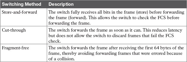
Figure Q-4 shows the idea of how OSPF advertises the default route, with the specific OSPF configuration. In this case, a company connects to an ISP with their Router R1. That router uses the OSPF default-information originate command (Step 1). As a result, the router advertises a default route using OSPF (Step 2) to the remote routers (B1, B2, and B3).
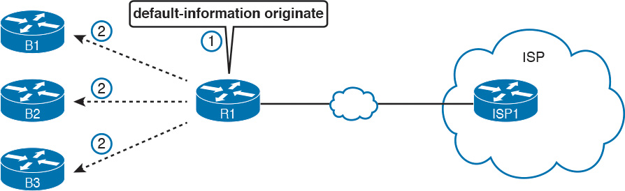
Figure Q-5 shows the default routes that result from OSPF’s advertisements in Figure Q-4. On the far left, the three branch routers all have OSPF-learned default routes pointing to R1. R1 itself also needs a default route, pointing to the ISP router, so that R1 can forward all Internet-bound traffic to the ISP.

Finally, this feature gives the engineer control over when the router originates this default route. First, R1 needs a default route, either defined as a static default route or learned from the ISP. The default-information originate command then tells the R1 to advertise a default route when its own default route is working, and to advertise it as down when its own default route fails.
Note
Interestingly, the default-information originate always router subcommand tells the router to always advertise the default route, no matter whether the router’s default route is working or not.
Note
The content under the heading “Name Resolution with DNS” was most recently published for the 100-101 Exam in 2013, in Chapter 18 of the CCENT/CCNA ICND1 100-101 Official Cert Guide. This short topic focuses on host name resolution.
Name Resolution with DNS
Consider the network topology in Figure Q-6 for the discussion that follows.

When looking at problems with hosts, you can and should check the DNS settings to find out what DNS server addresses the host tries to use. At the same time, the user at the host can make the host try to use DNS. For example:
![]() Open a web browser and type in the name of the web server. DNS resolves the name that sits between the // and the first /.
Open a web browser and type in the name of the web server. DNS resolves the name that sits between the // and the first /.
![]() Use a command like nslookup hostname, supported on most PC OSs, which sends a DNS Request to the DNS server, showing the results.
Use a command like nslookup hostname, supported on most PC OSs, which sends a DNS Request to the DNS server, showing the results.
Example Q-14 shows an example of the nslookup command that confirms that the host’s Domain Name System (DNS) server is set to 209.18.47.61, with the end of the output showing that the DNS request worked.
Example Q-14 nslookup Command (Mac)
Wendell-Odoms-iMac: wendellodom$ nslookup www.certskills.com
Server: 209.18.47.61
Address: 209.18.47.61#53
Non-authoritative answer:
www.certskills.com canonical name = certskills.com.
Name: certskills.com
Address: 173.227.251.150
And as a brief aside, note that routers and switches do have some settings related to DNS. However, these router and switch DNS settings only allow the router or switch to act as a DNS resolver (client). That is, the router and switch will use DNS messages to ask the DNS server to resolve the name into its matching IP address. The commands to configure how a router or switch will resolve host names into their matching addresses (all global commands) are
ip name-server server_IP...: Configure the IP addresses of up to six DNS servers in this one command.
ip host name address: Statically configure one name and matching IP address on this one router or switch. The local router/switch will use this IP address only if a command refers to the name.
no ip domain-lookup: Disable the DNS resolver function so that the router or switch does not attempt to ask a DNS server to resolve names. (The ip domain-lookup command, a default setting, enables the router to use a DNS server.)
Note
The content in this section did not appear in prior editions. It was planned for a prior edition and was not included for space. It is included here for those who may care.
IOS Reorders ACEs
Under some circumstances, IOS can appear to have changed your ACL. This behavior can be quite confusing to people just learning ACLs. This next topic points out two ways in which it appears that IOS is changing your ACL, describing what IOS is actually doing, and why neither of these apparent changes impact the logic of your ACL.
From the first moment that you begin to learn about ACLs, you hear facts like this:
![]() The order of the ACL statements—the access control entries (ACE)—are important, because IOS acts based on the first ACE matched in an ACL.
The order of the ACL statements—the access control entries (ACE)—are important, because IOS acts based on the first ACE matched in an ACL.
![]() If you ignored line numbers when configuring the ACL, IOS uses the order in which you typed the commands to determine the order to search the ACL ACEs.
If you ignored line numbers when configuring the ACL, IOS uses the order in which you typed the commands to determine the order to search the ACL ACEs.
![]() If you choose to configure line numbers, the order of the line numbers tells IOS what order to search the statements when matching the ACL.
If you choose to configure line numbers, the order of the line numbers tells IOS what order to search the statements when matching the ACL.
First, IOS can tell when the order of the statements could be changed for faster internal ACL processing, without changing the logic of the ACL. Sometimes, the order cannot be changed, and sometimes it can. Generally, the less overlap between the statements in the ACL, the more likely IOS can and will reorder the ACL.
As an example, consider the first three lines of ACL anyorder in Example Q-15. Each ACE matches one host.
Example Q-15 Example of IOS Reordering the ACEs in an ACL
R1# configure terminal
Enter configuration commands, one per line. End with CNTL/Z.
R1(config)# ip access-list standard anyorder
R1(config-std-nacl)# permit 9.9.9.1
R1(config-std-nacl)# permit 9.9.9.2
R1(config-std-nacl)# permit 9.9.9.3
R1(config-std-nacl)# ^Z
R1#
You could reorder the ACEs in the ACL in Example Q-15 and any other order would work the same way, because the matching logic does not overlap between the three statements. And because a reordering of these three ACEs would have no impact, IOS takes advantage of that fact and reorders the ACEs in the ACL. But why?
Cisco IOS examines and optimizes each ACL based on the router’s internal search algorithm when matching packets against the ACL. Cisco does not say much about the particulars of the internal algorithms. But more importantly, IOS only changes the order to optimize the search if that change has no impact on the ACL. Summarizing:

IOS may change the order of comparison for ACEs in an ACL, but only if that change does not impact the decision (the match) made by the ACL.
Continuing the example in Example Q-15, the person who created that ACL could have listed the individual ACEs in any order without changing the logic. However, as typed into configuration mode, the statements in that ACL have a specific order. IOS may prefer a different order. Example Q-16 shows excerpts from two show commands that shows how IOS reordered the sequence to optimize its own internal processing.
Example Q-16 Evidence of Reordering That Does Not Impact the ACL Decision
R1# show access-list anyorder
Standard IP access list anyorder
10 permit 9.9.9.1
30 permit 9.9.9.3
20 permit 9.9.9.2
R1# show running-config | section ip access-list standard anyorder
ip access-list standard anyorder
permit 9.9.9.1
permit 9.9.9.3
permit 9.9.9.2
R1#
When IOS reorders for internal processing, the literal order in the output of the show commands tells us the order IOS will use. For example, in this case, IOS will compare the statement with 9.9.9.1 first, then 9.9.9.3, and then 9.9.9.2. However, note that the ACL line numbers for each ACE did not change.
As one final comparison, when ACE matching logic overlaps, the order of the ACEs is important and IOS does not change the order. Example Q-17 shows an example. The ACL uses ACEs that match three overlapping groups: host 9.9.9.9, all addresses that begin 9.9.9, and all addresses that begin 9.9. Because these address ranges overlap, any reordering among these three ACEs would change the logic of the ACL. Notice that the show access-lists command at the end of the example confirms that IOS did not change the order of these ACEs; the order of lines in the output tells us the order IOS will use to process the ACL.
Example Q-17 ACL Example That Does Not Allow IOS to Reorder
R1# configure terminal
Enter configuration commands, one per line. End with CNTL/Z.
R1(config)# ip access-list standard thisorderonly
R1(config-std-nacl)# permit 9.9.9.9
R1(config-std-nacl)# deny 9.9.9.0 0.0.0.255
R1(config-std-nacl)# permit 9.9.0.0 0.0.255.255
R1(config-std-nacl)# ^Z
R1#
*Aug 20 14:17:52.247: %SYS-5-CONFIG_I: Configured from console by console
R1#
R1# show run | section ip access-list standard thisorderonly
ip access-list standard thisorderonly
permit 9.9.9.9
deny 9.9.9.0 0.0.0.255
permit 9.9.0.0 0.0.255.255
R1#
IOS Renumbers ACL Line Numbers, by 10s, at Reload
IOS enables you to edit an ACL in place. You can add ACL statements between others by referencing line numbers, delete single lines of ACLs using line numbers, and use any line numbers you would like to use.
Later, when you reload, IOS renumbers the line numbers sequentially, by 10s, starting at 10. Yep.
As it turns out, IOS does some subtle tricks with line numbers. The goal of the line numbers is to remember the relative order. IOS does that internally, and does not even store the line numbers in the configuration. Did you notice the fact that the show running-config output in the two previous examples does not even list the line numbers? That is because IOS records the relative order in the config files but not the literal line numbers.
This particular hidden behavior can be a little confusing when learning ACLs. You configure an ACL, you use line numbers, and maybe you insert a line with line number 15 in between lines 10 and 20. Great: that is what the line numbers are for. Later, you issue a copy running-config startup-config, turn off your lab gear, and start it up again the next day for more practice—and your ACL now lists new line numbers and that 15 you configured is gone. The ACL statement is still there; it just has a different line number.
The sequence at startup for IOS’s renumbering and reordering happens like this:
Step 1. At boot, find each ACL.
Step 2. Give each ACL entry a line number, by 10s, starting at 10, based on the relative order.
Step 3. After that, perform IOS reordering of the lines in the ACL.
Note
The content under the heading “NAT Overload (PAT) on Consumer Routers” was most recently published for the 100-101 Exam in 2013, in Chapter 24 of the CCENT/CCNA ICND1 100-101 Official Cert Guide. This short topic focuses on how consumer routers do NAT.
NAT Overload (PAT) on Consumer Routers
Consumer-grade Cisco routers enable many features by default, including NAT overload, or PAT. The strategy with consumer-grade routers allows the consumer to just physically install the router and cables, without needing to configure the router. This topic discusses how these consumer-grade routers work to enable PAT, even when using defaults.
First, as mentioned way back in Chapter 3, “Fundamentals of WANs,” products sold in the store as a “router” actually have many features: a router, a LAN switch, often with a wireless LAN access point, and a security firewall. They often include the PAT function as well. As for hardware, these routers have several RJ-45 ports labeled as “LAN”; these are ports for the LAN switch function. They also have one RJ-45 port labeled “WAN,” which is another Ethernet port that acts like a router interface, typically connected to a DSL or cable modem that in turn connects to the Internet, as shown in Figure Q-7.

To understand how a consumer router does PAT by default, you first must understand how it does DHCP. The router acts as a DHCP server on the LAN side, using a private IP network prechosen by the router vendor. (Cisco products often use private Class C network 192.168.1.0.) Then, on the WAN side, the router acts as a DHCP client, leasing an IP address from the ISP’s DHCP server. However, the address learned from the ISP is not a private IP address but a public IPv4 address, as shown in Figure Q-8.
Note
To make an enterprise-class router act like the router in Figure Q-8, on the WAN port, use the ip address dhcp interface subcommand. This command simply tells the router to learn its own interface IP address with DHCP. The DHCP server configuration would use the same commands detailed in Chapter 20, “DHCP and IP Networking on Hosts.”
By using DHCP on both the LAN and the WAN sides, a consumer router has created a perfect match of IP addresses to use PAT. The computers on the LAN all have private IP addresses, and the one WAN port has a public IP address. All the consumer router has to do is enable PAT, with the LAN side of the router as the NAT inside and the WAN port on the NAT outside, as shown in Figure Q-9.

Note
The content under the heading “Dynamic Routes with OSPFv3” was most recently published for the 100-101 Exam in 2013, in Chapter 29 of the CCENT/CCNA ICND1 100-101 Official Cert Guide. This short topic focuses on using OSPF to learn IPv6 routes.
Dynamic Routes with OSPFv3
Although static routes work, most internetworks use a dynamic routing protocol to learn the IPv6 routes for all subnets not connected to a local router. This last major section of the appendix looks at one IPv6 routing protocol—OSPF version 3—focusing on the similarities with OSPF version 2 and the configuration.
This section begins by working through some conceptual and theoretical details about OSPF version 3 (OSPFv3). After going through a short discussion of theory, this section walks you through the configuration, which is both different and simpler than the equivalent OSPFv2 configuration for IPv4. This section ends with many examples of show commands to find out whether OSPFv3 is working correctly, learning IPv6 routes.
Comparing OSPF for IPv4 and IPv6
As you might expect, OSPFv3—the version of OSPF that supports IPv6—works a lot like OSPFv2, which supports IPv4. The next few pages work through some of the terminology, concepts, similarities, and differences in how OSPF works for IPv6 versus IPv4.
OSPF Routing Protocol Versions and Protocols
First, when most engineers refer to “OSPF,” they most likely refer to OSPF as used with IPv4, and specifically, OSPF version 2 (OSPFv2). Once, there was an OSPF version 1, but OSPF version 2 (OSPFv2) followed soon afterward. When OSPF became widely used as an IPv4 routing protocol, back in the early to mid 1990s, everyone used OSPFv2 and not OSPFv1. So, even in the early days of OSPF, there was no need for people to talk about whether they used OSPFv1 or OSPFv2; everyone used OSPFv2 and just called it OSPF.
Next, consider the development of the original IPv6 protocols, back in early to mid 1990s. Beyond IPv6 itself, many other protocols needed to be updated to make IPv6 work: ICMP, TCP, UDP, and so on, including OSPF. When a working group updated OSPF to support IPv6, what did they call it? OSPFv3, of course.
Interestingly, OSPFv3 supports advertising IPv6 routes but not IPv4 routes. So, OSPFv3 does not attempt to add IPv6 support to the existing OSPFv2. Although the protocols share many similarities, think of OSPFv2 and OSPFv3 as different routing protocols: one for IPv4 routes (OSPFv2) and one for IPv6 routes (OSPFv3).
Because OSPFv3 advertises IPv6 routes, and only IPv6 routes, an enterprise network that uses a dual-stack strategy actually needs to run both OSPFv2 and OSPFv3 (assuming they use OSPF at all). Are their underlying concepts very similar? Yes. However, each router would run both an OSPFv2 and OSPFv3 routing protocol process, with both processes forming neighbor relationships, both sending database updates, and both calculating routes. So, a typical migration from an OSPFv2, IPv4-only enterprise network, to instead support a dual-stack IPv4/IPv6 approach (running both IPv4 and IPv6 on each host/router), would use these basic steps:
Step 1. Before IPv6, the company supports IPv4 using OSPFv2.
Step 2. When planning to add IPv6 support, the company plans to use a dual-stack approach, supporting both IPv4 and IPv6 routing on the routers in the enterprise network.
Step 3. To support IPv6 routing, companies add OSPFv3 configuration to all the routers, but they must keep the OSPFv2 configuration to continue to route IPv4 packets.
Other routing protocols followed a similar progression for updates to support IPv6, although with more unusual names. In the case of Routing Information Protocol (RIP), RIP has two versions that support IPv4, with the expected names of RIP version 1 (RIPv1) and RIP version 2 (RIPv2). To support IPv6, a working group created a new version of RIP, called RIP next generation (RIPng), with the name chosen in reference to the Star Trek TV series. (Yep.) Enhanced Interior Gateway Routing Protocol (EIGRP), as a Cisco-proprietary routing protocol, has always been known simply as EIGRP. However, to make discussions easier, some documents refer to EIGRP IPv4 support as EIGRP, and EIGRP for IPv6 as EIGRPv6.
Table Q-4 summarizes the terminology for these main three interior IP routing protocols.
Comparing OSPFv2 and OSPFv3
To the depth that this book discusses OSPF theory and concepts, OSPFv3 acts very much like OSPFv2. For example, both use link-state logic. Both use the same metric. And the list keeps getting longer, because the protocols do have many similarities. The following list notes many of the similarities for the features of OSPFv2 and OSPFv3:
![]() Both are link-state protocols.
Both are link-state protocols.
![]() Both use the same area design concepts and design terms.
Both use the same area design concepts and design terms.
![]() Both require that the routing protocol be enabled on an interface.
Both require that the routing protocol be enabled on an interface.
![]() Once enabled on an interface, both then attempt to discover neighbors connected to the data link connected to an interface.
Once enabled on an interface, both then attempt to discover neighbors connected to the data link connected to an interface.
![]() Both perform a check of certain settings before a router will become neighbors with another router. (The list of checks is slightly different between OSPFv2 and OSPFv3.)
Both perform a check of certain settings before a router will become neighbors with another router. (The list of checks is slightly different between OSPFv2 and OSPFv3.)
![]() After two routers become neighbors, both OSPFv2 and OSPFv3 proceed by exchanging the contents of their link-state databases (LSDB)—the link-state advertisements (LSA) that describe the network topology—between the two neighbors.
After two routers become neighbors, both OSPFv2 and OSPFv3 proceed by exchanging the contents of their link-state databases (LSDB)—the link-state advertisements (LSA) that describe the network topology—between the two neighbors.
![]() After all the LSAs have been exchanged, both OSPFv2 and OSPFv3 use the shortest path first (SPF) algorithm to calculate the best route to each subnet.
After all the LSAs have been exchanged, both OSPFv2 and OSPFv3 use the shortest path first (SPF) algorithm to calculate the best route to each subnet.
![]() Both use the same metric concept, based on the interface cost of each interface, with the same default cost values.
Both use the same metric concept, based on the interface cost of each interface, with the same default cost values.
![]() Both use LSAs to describe the topology, with some differences in how LSAs work.
Both use LSAs to describe the topology, with some differences in how LSAs work.
The biggest differences between OSPFv3 and the older OSPFv2 lay with internals and configuration. OSPFv3 changes the structure of some OSPF LSAs; however, these differences do not sit within the scope of this book. OSPFv3 uses a more direct approach to configuration, enabling OSPFv3 on each interface using an interface subcommand.
For later comparison to OSPFv3 configuration, Figure Q-10 shows the structure of the configuration for OSPFv2. It shows the fact that the OSPFv2 network subcommand—a subcommand in router configuration mode—refers to the IPv4 address on an interface, which then identifies the interface on which OSPFv2 should be enabled. In other words, the OSPFv2 configuration does not mention the interface directly.

OSPFv3 configuration directly enables OSPF on the interface by adding a subcommand in interface configuration mode to enable OSPFv3 on that interface. In fact, OSPFv3 does not use a network subcommand in router configuration mode. Instead, OSPFv3 uses the ipv6 ospf process-id area area-id interface subcommand, as shown in Figure Q-11. This command enables the listed OSPFv3 process on that interface and sets the OSPFv3 area.

Note
Cisco IOS actually supports configuration of OSPFv2 using the same style of commands shown for OSPFv3 in Figure Q-11 as well. IOS supports only the new, more direct configuration style for OSPFv3, as shown in the figure.
Now that you have a general idea about the similarities and differences between OSPFv3 and OSPFv2, the rest of this section shows examples of how to configure and verify OSPFv3.
Configuring Single-Area OSPFv3
OSPFv3 configuration requires some basic steps: pick and configure a process ID, and enable the process on each interface, while assigning the correct OSPF area to each interface. These details should be listed in any planning information. Also, this book uses single-area designs only, so all the interfaces should be assigned to the same area.
The one potential configuration issue is the OSPFv3 router ID (RID).
For review, OSPFv2 uses a 32-bit RID, chosen when the OSPF process initializes. That is, when OSPF is first configured, or later, when the router is reloaded, the OSPFv2 process chooses a number to use as its RID. The OSPFv2 process chooses its RID using this list until it finds a RID:
1. If the router-id rid OSPF subcommand is configured, use this value, and ignore interface IPv4 addresses.
2. If the router ID is not set with the router-id command, check any loopback interfaces that have an IPv4 address configured and an interface status of up. Among these, pick the highest numeric IP address.
3. If neither of the first two items supply a router ID, the router picks the highest numeric IPv4 address from all other interfaces whose interface status code (first status code) is up. (In other words, an interface in an up/down state will be included by OSPF when choosing its router ID.)
Interestingly, OSPFv3 also uses a 32-bit RID, using the exact same rules as OSPFv2. The number is typically listed in dotted-decimal notation (DDN). That is, OSPFv3, which supports IPv6, has a router ID that looks like an IPv4 address.
Using the same RID selection rules for OSPFv3 as for OSPFv2 leaves open one unfortunate potential misconfiguration: A router that does not use the OSPFv3 router-id command, and does not have any IPv4 addresses configured, cannot choose a RID. If the OSPFv3 process does not have an RID, the process cannot work correctly, form neighbor relationships, or exchange routes.
This problem can be easily solved. When configuring OSPFv3, if the router does not have any IPv4 addresses, make sure to configure the RID using the router-id router subcommand.
Beyond that one small issue, the OSPFv3 configuration is relatively simple. The following list summarizes the configuration steps and commands for later reference and study, with examples to follow:
Step 1. Create an OSPFv3 process number and enter OSPF configuration mode for that process, using the ipv6 router ospf process-id global command.
Step 2. Ensure that the router has an OSPF router ID, through either
A. Configuring the router-id id-value router subcommand
B. Preconfiguring an IPv4 address on any loopback interface whose line status is up
C. Preconfiguring an IPv4 address on any working interface whose line status is up
Step 3. Configure the ipv6 ospf process-id area area-number command on each interface on which OSPFv3 should be enabled, to both enable OSPFv3 on the interface and set the area number for the interface.
OSPFv3 Single-Area Configuration Example
Figure Q-12 shows the details of an internetwork used for an OSPFv3 configuration example. The figure shows a single area (area 0). Also, note that Routers R2 and R3 connect to the same VLAN and IPv6 prefix on the right.
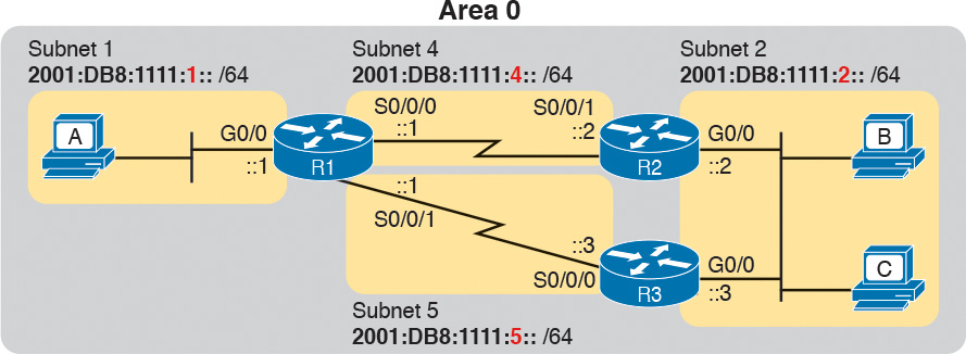
The upcoming OSPFv3 configuration example uses the following requirements:
![]() All interfaces will be in area 0, so all the ipv6 ospf process-id area area-number commands will refer to area 0.
All interfaces will be in area 0, so all the ipv6 ospf process-id area area-number commands will refer to area 0.
![]() Each router uses a different OSPF process ID number, just to emphasize the point that the process IDs do not have to match on neighboring OSPFv3 routers.
Each router uses a different OSPF process ID number, just to emphasize the point that the process IDs do not have to match on neighboring OSPFv3 routers.
![]() Each router sets its router ID directly with the router-id command to an obvious number (1.1.1.1, 2.2.2.2, and 3.3.3.3 for R1, R2, and R3, respectively).
Each router sets its router ID directly with the router-id command to an obvious number (1.1.1.1, 2.2.2.2, and 3.3.3.3 for R1, R2, and R3, respectively).
![]() The routers do not use IPv4.
The routers do not use IPv4.
To begin, Example Q-18 shows an excerpt from R1’s show running-config command before adding the OSPFv3 configuration with the ipv6 unicast-routing command, plus an ipv6 address command on each interface.
Example Q-18 R1 IPv6 Configuration Reference (Before Adding OSPFv3 Configuration)
ipv6 unicast-routing
!
interface serial0/0/0
no ip address
ipv6 address 2001:db8:1111:4::1/64
!
interface serial0/0/1
no ip address
ipv6 address 2001:db8:1111:5::1/64
!
interface GigabitEthernet0/0
no ip address
ipv6 address 2001:db8:1111:1::1/64
Example Q-19 begins to show the OSPFv3 configuration, starting on Router R1. Note that at this point, Router R1 has no IPv4 addresses configured, so R1 cannot possibly choose an OSPFv3 RID; it must rely on the configuration of the router-id command. Following the example in sequence, the following occurs:
Step 1. The engineer adds the ipv6 router ospf 1 global command, creating the OSPFv3 process.
Step 2. The router tries to allocate an OSPFv3 RID and fails, so it issues an error message.
Step 3. The engineer adds the router-id 1.1.1.1 command to give R1’s OSPFv3 process an RID.
Step 4. The engineer adds ipv6 ospf 1 area 0 commands to all three interfaces.
Example Q-19 Additional Configuration on R1 to Enable OSPFv3 on Three Interfaces
R1# configure terminal
Enter configuration commands, one per line. End with CNTL/Z.
R1(config)# ipv6 router ospf 1
Jan 4 21:03:50.622: %OSPFv3-4-NORTRID: OSPFv3 process 1 could not pick a router-id,
please configure manually
R1(config-rtr)# router-id 1.1.1.1
R1(config-rtr)#
R1(config-rtr)# interface serial0/0/0
R1(config-if)# ipv6 ospf 1 area 0
R1(config-if)# interface serial0/0/1
R1(config-if)# ipv6 ospf 1 area 0
R1(config-if)# interface GigabitEthernet0/0
R1(config-if)# ipv6 ospf 1 area 0
R1(config-if)# end
R1#
When looking at the configuration on a single OSPFv3 router, only two other types of parameters can be an issue: the OSPF process ID and the area number. When checking an OSPFv3 configuration for errors, first check the process ID numbers and make sure that all the values match on that router. For example, the ipv6 router ospf process-id command’s process ID should match all the ipv6 ospf process-id ... interface subcommands. The other value, the area number, simply needs to match the planning diagram that shows which interfaces should be in which area.
When comparing two neighboring routers, some parameters must match or the routers will not become neighbors. Troubleshooting these kinds of problems sits within the scope of the 200-101 ICND2 exam, not the 100-101 ICND1 exam. However, the one big difference between OSPFv2 and OSPFv3 in this neighbor checklist is that OSPFv3 neighbors do not have to have IPv6 prefixes (subnets) or prefix lengths that match. Otherwise, OSPFv3 neighbors must match with items such as both routers being in the same area, having the same Hello interval and the same dead interval.
Example Q-20 shows a completed configuration for Router R2. In this case, Router R2 uses a different OSPF process ID than R1; the process IDs on neighbors do not have to match with OSPFv2 or OSPFv3. R2 creates its OSPFv3 process (2), sets its RID (2.2.2.2), and enables OSPFv3 on all three of its interfaces with the ipv6 ospf 2 area 0 interface subcommand.
Example Q-20 Complete IPv6 Configuration, Using OSPFv3, on Router R2
ipv6 unicast-routing
!
ipv6 router ospf 2
router-id 2.2.2.2
!
interface serial0/0/1
ipv6 address 2001:db8:1111:4::2
ipv6 ospf 2 area 0
!
interface GigabitEthernet0/0
ipv6 address 2001:db8:1111:2::2
ipv6 ospf 2 area 0
OSPFv3 Passive Interfaces
Like OSPFv2, OSPFv3 can be configured to make interfaces passive. Some IPv6 subnets have only one router connected to the subnet. In those cases, the router needs to enable OSPFv3 on the interface, so that the router advertises about the connected subnet, but the router does not need to attempt to discover OSPFv3 neighbors on the interface. In those cases, the engineer can configure the interface as on OSPFv3 passive interface, telling the router to do the following:
![]() Quit sending OSPF Hellos on the interface
Quit sending OSPF Hellos on the interface
![]() Ignore received Hellos on the interface
Ignore received Hellos on the interface
![]() Do not form neighbor relationships over the interface
Do not form neighbor relationships over the interface
![]() Continue to advertise about any subnets connected to the interface
Continue to advertise about any subnets connected to the interface
Interestingly, passive interface configuration works the same for both OSPFv2 and OSPFv3. For example, in the configuration example based on Figure Q-12, only R1 connects to the LAN subnet on the left side of the figure, so R1’s G0/0 interface could be made passive to OSPFv3. To do so, the engineer could add the passive-interface gigabitethernet0/0 subcommand in OSPFv3 configuration mode on Router R1.
Verifying OSPFv3 Status and Routes
To verify whether OSPFv3 works, you can take two different approaches. You can start at the end, looking at the IPv6 routes added by OSPFv3. If the correct routes show up in the correct routers’ routing tables, OSPFv3 must be working correctly. Alternatively, you can proceed in the same order that OSPF uses to build the routes: First confirm the configuration settings, then look at the OSPF neighbors, then the OSPF database, and finally look at the routes OSPF added to the routing tables.
When speed matters, look at the routing table first. However, for the sake of learning, it helps to walk through the steps from start to finish, working through a variety of OSPFv3 show commands. The rest of this section works through several OSPFv3 show commands, in this order:
![]() Verifying the configuration settings (OSPFv3 process and interfaces)
Verifying the configuration settings (OSPFv3 process and interfaces)
![]() Verifying OSPFv3 neighbors
Verifying OSPFv3 neighbors
![]() Verifying the OSPFv3 link-state database (LSDB) and LSAs
Verifying the OSPFv3 link-state database (LSDB) and LSAs
![]() Verifying OSPFv3 routes
Verifying OSPFv3 routes
This section happens to mention a wide variety of OSPFv3 show commands that have a matching and similar OSPFv2 show command. Table Q-5 lists these show commands for easier reference and study.

Note that all the OSPFv3 commands use the exact same commands as those for IPv4, except they use ipv6 instead of the ip parameter.
Verifying OSPFv3 Configuration Settings
To verify the OSPFv3 configuration on a router, a simple show running-config command works well. However, in some cases in real life, and on the exams with many Simlet questions, you might not be allowed to enter enable mode to use commands like show running-config. In those cases, you can re-create the OSPFv3 configuration using several show commands.
To start re-creating the OSPFv3 configuration, look at the output of the show ipv6 ospf command. This command lists information about the OSPFv3 process itself. In fact, the first line of output, highlighted in Example Q-21, tells you the following facts about the configuration:
![]() The router has been configured with OSPFv3 process ID 1, meaning the ipv6 router ospf 1 command is configured.
The router has been configured with OSPFv3 process ID 1, meaning the ipv6 router ospf 1 command is configured.
![]() The router uses router ID 1.1.1.1, which means either the router-id 1.1.1.1 command is configured or the ip address 1.1.1.1 mask command is configured on some interface on the router.
The router uses router ID 1.1.1.1, which means either the router-id 1.1.1.1 command is configured or the ip address 1.1.1.1 mask command is configured on some interface on the router.
Example Q-21 Verifying OSPFv3 Process Configuration
R1# show ipv6 ospf
Routing Process "ospfv3 1" with ID 1.1.1.1
Event-log enabled, Maximum number of events: 1000, Mode: cyclic
Initial SPF schedule delay 5000 msecs
Minimum hold time between two consecutive SPFs 10000 msecs
Maximum wait time between two consecutive SPFs 10000 msecs
Minimum LSA interval 5 secs
Minimum LSA arrival 1000 msecs
LSA group pacing timer 240 secs
Interface flood pacing timer 33 msecs
Retransmission pacing timer 66 msecs
Number of external LSA 0. Checksum Sum 0x000000
Number of areas in this router is 1. 1 normal 0 stub 0 nssa
Graceful restart helper support enabled
Reference bandwidth unit is 100 mbps
Area BACKBONE(0)
Number of interfaces in this area is 3
SPF algorithm executed 4 times
Number of LSA 13. Checksum Sum 0x074B38
Number of DCbitless LSA 0
Number of indication LSA 0
Number of DoNotAge LSA 0
Flood list length 0
The highlights toward the end of Example Q-21 give some hints about the rest of the configuration but not enough detail to list every part of the remaining OSPFv3 configuration. The highlighted lines mention three interfaces are in “this area” and that the area is backbone area 0. All these messages sit under the heading line at the top of the example, for OSPFv3 process 1. These facts together tell us that this router (R1) uses the following configuration:
![]() Interface subcommand ipv6 ospf 1 area 0.
Interface subcommand ipv6 ospf 1 area 0.
![]() The router uses this interface subcommand on three interfaces.
The router uses this interface subcommand on three interfaces.
However, the show ipv6 ospf command does not identify the interfaces on which OSPFv3 is working. To find those interfaces, use either of the two commands in Example Q-22. Focusing first on the show ipv6 ospf interface brief command, this command lists one line for each interface on which OSPFv3 is enabled. Each line lists the interface, the OSPFv3 process ID (under the heading PID), the area assigned to the interface, and the number of OSPFv3 neighbors (Nbrs heading) known out that interface.
Example Q-22 Verifying OSPFv3 Interfaces
R1# show ipv6 ospf interface brief
Interface PID Area Intf ID Cost State Nbrs F/C
Gi0/0 1 0 3 1 DR 0/0
Se0/0/1 1 0 7 64 P2P 1/1
Se0/0/0 1 0 6 64 P2P 1/1
R1# show ipv6 protocols
IPv6 Routing Protocol is "connected"
IPv6 Routing Protocol is "ND"
IPv6 Routing Protocol is "ospf 1"
Interfaces (Area 0):
GigabitEthernet0/0
Serial0/0/1
Serial0/0/0
Redistribution:
None
Note
Just as with the show ip ospf interface brief command, the show ipv6 ospf interface brief command lists both nonpassive and passive OSPFv3 interfaces.
The second half of the output in Example Q-22, listing the show ipv6 protocols command, lists information about every source of IPv6 routes on the router. This command lists noticeably less detail about OSPFv3 than the show ip protocol command lists about OSPFv2. However, both commands list the interfaces on which OSPFv3 is enabled.
Both of the commands in Example Q-22 give enough information to predict that this router (R1) has an ipv6 ospf 1 area 0 subcommand under three interfaces: G0/0, S0/0/0, and S0/0/1.
Verifying OSPFv3 Neighbors
Verifying OSPFv3 neighbors requires a brief look at a single command: show ipv6 ospf neighbor. This command lists one line per neighbor, listing key facts about that neighbor. In particular, it lists the neighbor’s RID, the local router’s interface through which that neighbor is reached, and the status of the neighbor relationship.
In the OSPFv3 example used in this chapter, each router should have two neighbor relationships. R1 has two serial links, one each to Routers R2 and R3, so R1 will form a neighbor relationship with each of these routers. R2 and R3 both connect to the same IPv6 subnet over a LAN, and will form a neighbor relationship over that LAN. Figure Q-13 shows the expected OSPFv3 neighbor relationships.

Figure Q-13 Expected OSPFv3 Neighbor Relationships Compared to Figure Q-12
Example Q-23 shows the OSPFv3 neighbor relationships on Routers R1 and R2. The highlighted portions point out the basics, with the neighboring routers’ RIDs, local interface, and state. The “FULL” state means that the neighbor relationship is working, and that the neighbors have “fully” completed the exchange of LSAs.
Example Q-23 Verifying OSPFv3 Neighbors on Routers R1 and R2
! The first command is from router R1, listing R2 and R3
R1# show ipv6 ospf neighbor
Neighbor ID Pri State Dead Time Interface ID Interface
3.3.3.3 0 FULL/ - 00:00:39 6 Serial0/0/1
2.2.2.2 0 FULL/ - 00:00:31 7 Serial0/0/0
! The next command is from router R2, listing R1 and R3
R2# show ipv6 ospf neighbor
Neighbor ID Pri State Dead Time Interface ID Interface
1.1.1.1 0 FULL/ - 00:00:39 6 Serial0/0/1
3.3.3.3 1 FULL/DR 00:00:33 3 GigabitEthernet0/0
Before speeding along to the next topic, take a moment to look again at the output in Example Q-23. Do you see anything in the output that makes you think of IPv6 instead of IPv4? OSPFv3 uses 32-bit RIDs, listed in dotted-decimal notation, and it lists the IPv6 interface ID, as opposed to the full IPv4 address, in the fifth column of output.
Examining the OSPFv3 Database
OSPFv3 does differ from OSPFv2 with the theory and details of OSPF LSAs. However, this book mostly ignores LSA details, with the ICND2 book discussing LSAs in a small amount of detail. To understand the differences between OSPFv2 and OSPFv3, the discussion would need to be much deeper.
However, an easy way to do a basic check of the LSDB is to check for Type 1 router LSAs. Both OSPFv2 and OSPFv3 use a Type 1 LSA for every router, with the LSA describing the router itself. The LSA has an identifier equal to the RID of that router. Inside an area, the LSDB should contain one Type 1 LSA for every router in the area. Example Q-24 shows the first section of output from the show ipv6 ospf database command and tells you whether a router has learned the Type 1 Router LSA from all the routers.
Example Q-24 Verifying OSPFv3 LSDB on R1
R2# show ipv6 ospf database
OSPFv3 Router with ID (2.2.2.2) (Process ID 2)
Router Link States (Area 0)
ADV Router Age Seq# Fragment ID Link count Bits
1.1.1.1 452 0x80000002 0 2 None
2.2.2.2 456 0x80000004 0 2 None
3.3.3.3 457 0x80000005 0 2 None
! Lines omitted for brevity
The example shows three lines of data under the heading lines in the section titled “Router Link States.” This section shows data about the Type 1 Router LSAs. In that section, the heading “ADV Router” refers to the router that advertised the LSA. In this case, R1 (RID 1.1.1.1) knows its own Type 1 LSA, plus R2’s (RID 2.2.2.2) and R3’s (RID 3.3.3.3).
Examining IPv6 Routes Learned by OSPFv3
Finally, the real proof of whether OSPFv3 works is whether the routers learn and add any IPv6 routes to the IPv6 routing table. This section completes the verification process with a look at the IPv6 routes added by OSPFv3.
When working correctly, OSPFv3 routers learn enough information to create routes for all IPv6 prefixes (subnets) in the internetwork. The one big difference as compared with OSPFv2 is that OSPFv3-learned routes use a link-local next-hop address. For example, in the internetwork shown in Figure Q-14, which is the same design used for the OSPFv3 configuration example, R2 adds a route to subnet 1 on the left (subnet 2001:DB8:1111:1::/64). R2 uses R1’s link-local address as the next-hop address, as shown in the figure.

Example Q-25 lists the output from the show ipv6 route ospf command on Router R2, for the route highlighted in Figure Q-14. Of particular importance, note
![]() Code letter O meaning OSPF
Code letter O meaning OSPF
![]() In brackets, 110, the administrative distance of OSPF, and 65, the metric for this route
In brackets, 110, the administrative distance of OSPF, and 65, the metric for this route
![]() The fact that the route lists both the link-local address and the outgoing interface
The fact that the route lists both the link-local address and the outgoing interface
Example Q-25 OSPFv3 Routes on Router R2
R2# show ipv6 route ospf
IPv6 Routing Table - default - 9 entries
! Legend omitted for brevity
O 2001:DB8:1111:1::/64 [110/65]
via FE80::FF:FE00:1, Serial0/0/1
O 2001:DB8:1111:5::/64 [110/65]
via FE80::FF:FE00:3, GigabitEthernet0/0