Chapter 11. Generic Algorithms
CONTENTS
Section 11.2 A First Look at the Algorithms 395
Section 11.3 Revisiting Iterators 405
Section 11.4 Structure of Generic Algorithms 419
Section 11.5 Container-Specific Algorithms 421
The library containers define a surprisingly small set of operations. Rather than adding lots of functionality to the containers, the library instead provides a set of algorithms, most of which are independent of any particular container type. These algorithms are generic: They operate on different types of containers and on elements of various types.
The generic algorithms, and a more detailed look at iterators, form the subject matter of this chapter.
The standard containers define few operations. For the most part they allow us to add and remove elements; to access the first or last element; to obtain and in some cases reset the size of the container; and to obtain iterators to the first and one past the last element.
We can imagine many other useful operations one might want to do on the elements of a container. We might want to sort a sequential container, or find a particular element, or find the largest or smallest element, and so on. Rather than define each of these operations as members of each container type, the standard library defines a set of generic algorithms: “algorithms” because they implement common operations; and “generic” because they operate across multiple container types—not only library types such as vector or list, but also the built-in array type, and, as we shall see, over other kinds of sequences as well. The algorithms also can be used on container types we might define ourselves, as long as our types conform to the standard library conventions.
Most of the algorithms operate by traversing a range of elements bounded by two iterators. Typically, as the algorithm traverses the elements in the range, it operates on each element. The algorithms obtain access to the elements through the iterators that denote the range of elements to traverse.
11.1 Overview
Suppose we have a vector of ints, named vec, and we want to know if it holds a particular value. The easiest way to answer this question is to use the library find operation:

The call to find takes two iterators and a value. It tests each element in the range (Section 9.2.1, p. 314) denoted by its iterator arguments. As soon as it sees an element that is equal to the given value, find returns an iterator referring to that element. If there is no match, then find returns its second iterator to indicate failure. We can test whether the return is equal to the second argument to determine whether the element was found. We do this test in the output statement, which uses the conditional operator (Section 5.7, p. 165) to report whether the value was found.
Because find operates in terms of iterators, we can use the same find function to look for values in any container. For example, we can use find to look for a value in a list of int named lst:
Except for the type of result and the iterators passed to find, this code is identical to the program that used find to look at elements of a vector.
Similarly, because pointers act like iterators on built-in arrays, we can use find to look in an array:

Here we pass a pointer to the first element in ia and another pointer that is six elements past the start of ia (that is, one past the last element of ia). If the pointer returned is equal to ia + 6 then the search is unsuccessful; otherwise, the pointer points to the value that was found.
If we wish to pass a subrange, we pass iterators (or pointers) to the first and one past the last element of that subrange. For example, in this invocation of find, only the elements ia [1] and ia [2] are searched:
// only search elements ia[1] and ia[2]
int *result = find(ia + 1, ia + 3, search_value);
How the Algorithms Work
Each generic algorithm is implemented independently of the individual container types. The algorithms are also largely, but not completely, independent of the types of the elements that the container holds. To see how the algorithms work, let’s look a bit more closely at find. Its job is to find a particular element in an unsorted collection of elements. Conceptually the steps that find must take include:
- Examine each element in turn.
- If the element is equal to the value we want, then return an iterator that refers to that element.
- Otherwise, examine the next element, repeating step 2 until either the value is found or all the elements have been examined.
- If we have reached the end of the collection and we have not found the value, return a value that indicates that the value was not found.
The Standard Algorithms Are Inherently Type-Independent
The algorithm, as we’ve stated it, is independent of the type of the container: Nothing in our description depends on the container type. Implicitly, the algorithm does have one dependency on the element type: We must be able to compare elements. More specifically, the requirements of the algorithm are:
- We need a way to traverse the collection: We need to be able to advance from one element to the next.
- We need to be able to know when we have reached the end of the collection.
- We need to be able to compare each element to the value we want.
- We need a type that can refer to an element’s position within the container or that can indicate that the element was not found.
Iterators Bind Algorithms to Containers
The generic algorithms handle the first requirement, container traversal, by using iterators. All iterators support the increment operator to navigate from one element to the next, and the dereference operator to access the element value. With one exception that we’ll cover in Section 11.3.5 (p. 416), the iterators also support the equality and inequality operators to determine whether two iterators are equal.
For the most part, the algorithms each take (at least) two iterators that denote the range of elements on which the algorithm is to operate. The first iterator refers to the first element, and the second iterator marks one past the last element. The element addressed by the second iterator, sometimes referred to as the off-the-end iterator, is not itself examined; it serves as a sentinel to terminate the traversal.
The off-the-end iterator also handles requirement 4 by providing a convenient return value that indicates that the search element wasn’t found. If the value isn’t found, then the off-the-end iterator is returned; otherwise, the iterator that refers to the matching element is returned.
Requirement 3, value comparison, is handled in one of two ways. By default, the find operation requires that the element type define operator ==. The algorithm uses that operator to compare elements. If our type does not support the == operator, or if we wish to compare elements using a different test, we can use a second version of find. That version takes an extra argument that is the name of a function to use to compare the elements.
The algorithms achieve type independence by never using container operations; rather, all access to and traversal of the elements is done through the iterators. The actual container type (or even whether the elements are stored in a container) is unknown.
The library provides more than 100 algorithms. Like the containers, the algorithms have a consistent architecture. Understanding the design of the algorithms makes learning and using them easier than memorizing all 100+ algorithms. In this chapter we’ll both illustrate the use of the algorithms and describe the unifying principles used by the library algorithms. Appendix A lists all the algorithms classified by how they operate.
11.2 A First Look at the Algorithms
Before covering the structure of the algorithms library, let’s look at a couple of examples. We’ve already seen the use of find; in this section we’ll use a few additional algorithms. To use a generic algorithm, we must include the algorithm header:
#include <algorithm>
The library also defines a set of generalized numeric algorithms, using the same conventions as the generic algorithms. To use these algorithms we include the numeric header:
#include <numeric>
With only a handful of exceptions, all the algorithms operate over a range of elements. We’ll refer to this range as the “input range.” The algorithms that take an input range always use their first two parameters to denote that range. These parameters are iterators used to denote the first and one past the last element that we want to process.
Although most algorithms are similar in that they operate over an input range, they differ in how they use the elements in that range. The most basic way to understand the algorithms is to know whether they read elements, write elements, or rearrange the order of the elements. We’ll look at samples of each kind of algorithm in the remainder of this section.
11.2.1 Read-Only Algorithms
A number of the algorithms read, but never write to, the elements in their input range. find is one such algorithm. Another simple, read-only algorithm is accumulate, which is defined in the numeric header. Assuming vec is a vector of int values, the following code
// sum the elements in vec starting the summation with the value 42
int sum = accumulate(vec.begin(), vec.end(), 42);
sets sum equal to the sum of the elements in vec plus 42. accumulate takes three parameters. The first two specify a range of elements to sum. The third is an initial value for the sum. The accumulate function sets an internal variable to the initial value. It then adds the value of each element in the range to that initial value. The algorithm returns the result of the summation. The return type of accumulate is the type of its third argument.

The third argument, which specifies the starting value, is necessary because accumulate knows nothing about the element types that it is accumulating. Therefore, it has no way to invent an appropriate starting value or associated type.
There are two implications of the fact that accumulate doesn’t know about the types over which it sums. First, we must pass an initial starting value because otherwise accumulate cannot know what starting value to use. Second, the type of the elements in the container must match or be convertible to the type of the third argument. Inside accumulate, the third argument is used as the starting point for the summation; the elements in the container are successively added into this sum. It must be possible to add the element type to the type of the sum.
As an example, we could use accumulate to concatenate the elements of a vector of strings:
// concatenate elements from v and store in sum
string sum = accumulate(v.begin(), v.end(), string(""));
The effect of this call is to concatenate each element in vec onto a string that starts out as the empty string. Note that we explicitly create a string as the third parameter. Passing a character-string literal would be a compile-time error. If we passed a string literal, the summation type would be const char* but the string addition operator (Section 3.2.3, p. 86) for operands of type string and const char* yields a string not a const char*.
Using find_first_of
In addition to find, the library defines several other, more complicated searching algorithms. Several of these are similar to the find operations of the string class (Section 9.6.4, p. 343). One such is find_first_of. This algorithm takes two pairs of iterators that denote two ranges of elements. It looks in the first range for a match to any element from the second range and returns an iterator denoting the first element that matches. If no match is found, it returns the end iterator of the first range. Assuming that roster1 and roster2 are two lists of names, we could use find_first_of to count how many names are in both lists:

The call to find_first_of looks for any element in roster2 that matches an element from the first range—that is, it looks for an element in the range from it to roster1.end(). The function returns the first element in that range that is also in the second range. On the first trip through the while, we look in the entire range of roster1. On second and subsequent trips, we look in that part of roster1 that has not already been matched.
In the condition, we check the return from find_first_of to see whether we found a matching name. If we got a match, we increment our counter. We also increment it so that it refers to the next element in roster1. We know we’re done when find_first_of returns roster1.end(), which it does if there is no match.
11.2.2 Algorithms that Write Container Elements
Some algorithms write element values. When using algorithms that write elements, we must take care to ensure that the sequence into which the algorithm writes is at least as large as the number of elements being written.
Some algorithms write directly into the input sequence. Others take an additional iterator that denotes a destination. Such algorithms use the destination iterator as a place in which to write output. Still a third kind writes a specified number of elements to some sequence.
Writing to the Elements of the Input Sequence
The algorithms that write to their input sequence are inherently safe—they write only as many elements as are in the specified input range.
A simple example of an algorithm that writes to its input sequence is fill:
fill takes a pair of iterators that denote a range in which to write copies of its third parameter. It executes by setting each element in the range to the given value. Assuming that the input range is valid, then the writes are safe. The algorithm writes only to elements known to exist in the input range itself.
Algorithms Do Not Check Write Operations
The fill_n function takes an iterator, a count, and a value. It writes the specified number of elements with the given value starting at the element referred to by the iterator. The fill_n function assumes that it is safe to write the specified number of elements. It is a fairly common beginner mistake to call fill_n (or similar algorithms that write to elements) on a container that has no elements:

This call to fill_n is a disaster. We specified that ten elements should be written, but there are no such elements— vec is empty. The result is undefined and will probably result in a serious run-time failure.

Algorithms that write a specified number of elements or that write to a destination iterator do not check whether the destination is large enough to hold the number of elements being written.
Introducing back_inserter
One way to ensure that an algorithm has enough elements to hold the output is to use an insert iterator. An insert iterator is an iterator that adds elements to the underlying container. Ordinarily, when we assign to a container element through an iterator, we assign to the element to which the iterator refers. When we assign through an insert iterator, a new element equal to the right-hand value is added to the container.
We’ll have more to say about insert iterators in Section 11.3.1 (p. 406). However, in order to illustrate how to safely use algorithms that write to a container, we will use back_inserter. Programs that use back_inserter must include the iterator header.
The back_inserter function is an iterator adaptor. Like the container adaptors (Section 9.7, p. 348), an iterator adaptor takes an object and generates a new object that adapts the behavior of its argument. In this case, the argument to back_inserter is a reference to a container. back_inserter generates an insert iterator bound to that container. When we attempt to assign to an element through that iterator, the assignment calls push_back to add an element with the given value to the container. We can use back_inserter to generate an iterator to use as the destination in fill_n:
Now, each time fill_n writes a value, it will do so through the insert iterator generated by back_inserter. The effect will be to call push_back on vec, adding ten elements to the end of vec, each of which has the value 0.
Algorithms that Write to a Destination Iterator
A third kind of algorithm writes an unknown number of elements to a destination iterator. As with fill_n, the destination iterator refers to the first element of a sequence that will hold the output. The simplest such algorithm is copy. This algorithm takes three iterators: The first two denote an input range and the third refers to an element in the destination sequence. It is essential that the destination passed to copy be at least as large as the input range. Assuming ilst is a list holding ints, we might copy it into a vector:

copy reads elements from the input range, copying them to the destination.
Of course, this example is a bit inefficient: Ordinarily if we want to create a new container as a copy of an existing container, it is better to use an input range directly as the initializer for a newly constructed container:
// better way to copy elements from ilst
vector<int> ivec(ilst.begin(), ilst.end());
Algorithm _copy Versions
Several algorithms provide so-called “copying” versions. These algorithms do some processing on the elements of their input sequence but do not change the original elements. Instead, a new sequence is written that contains the result of processing the elements of the original.
The replace algorithm is a good example. This algorithm reads and writes to an input sequence, replacing a given value by a new value. The algorithm takes four parameters: a pair of iterators denoting the input range and a pair of values. It substitutes the second value for each element that is equal the first:
// replace any element with value of 0 by 42
replace(ilst.begin(), ilst.end(), 0, 42);
This call replaces all instances of 0 by the 42. If we wanted to leave the original sequence unchanged, we would call replace_copy. That algorithm takes a third iterator argument denoting a destination in which to write the adjusted sequence:

After this call, ilst is unchanged, and ivec contains a copy of ilst with the exception that every element in ilst with the value 0 has the value 42 in ivec.
11.2.3 Algorithms that Reorder Container Elements
Suppose we want to analyze the words used in a set of children’s stories. For example, we might want know how many words contain six or more characters. We want to count each word only once, regardless of how many times it appears or whether it appears in multiple stories. We’d like to be able to print the words in size order, and we want the words to be in alphabetic order within a given size.
We’ll assume that we have read our input and stored the text of each book in a vector of strings named words. How might we solve the part of the problem that involves counting word occurrences? To solve this problem, we’d need to:
- Eliminate duplicate copies of each word
- Order the words based on size
- Count the words whose size is 6 or greater
Exercises Section 11.2.2
Exercise 11.6: Using fill_n, write a program to set a sequence of int values to 0.
Exercise 11.7: Determine if there are any errors in the following programs and, if so, correct the error(s):

Exercise 11.8: We said that algorithms do not change the size of the containers over which they operate. Why doesn’t the use of back_inserter invalidate this claim?
We can use generic algorithms in each of these steps.
For purposes of illustration, we’ll use the following simple story as our input:
the quick red fox jumps over the slow red turtle
Given this input, our program should produce the following output:
1 word 6 characters or longer
Eliminating Duplicates
Assuming our input is in a vector named words, our first subproblem is to eliminate duplicates from the words:
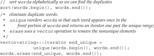
Our input vector contains a copy of every word used in each story. We start by sorting this vector. The sort algorithm takes two iterators that denote the range of elements to sort. It uses the < operator to compare the elements. In this call we ask that the entire vector be sorted.
After the call to sort, our vector elements are ordered:
fox jumps over quick red red slow the the turtle
Note that the words red and the are duplicated.
Using unique
Once words is sorted, our problem is to keep only one copy of each word that is used in our stories. The unique algorithm is well suited to this problem. It takes two iterators that denote a range of elements. It rearranges the elements in the input range so that adjacent duplicated entries are eliminated and returns an iterator that denotes the end of the range of the unique values.
After the call to unique, the vector holds
words
Note that the size of words is unchanged. It still has ten elements; only the order of these elements has changed. The call to unique “removes” adjacent duplicates. We put remove in quotes because unique doesn’t remove any elements. Instead, it overwrites adjacent duplicates so that the unique elements are copied into the front of the sequence. The iterator returned by unique denotes one past the end of the range of unique elements.
Using Container Operations to Remove Elements
If we want to eliminate the duplicate items, we must use a container operation, which we do in the call to erase. This call erases the elements starting with the one to which end_unique refers through the end of words. After this call, words contains the eight unique words from the input.
Algorithms never directly change the size of a container. If we want to add or remove elements, we must use a container operation.
It is worth noting that this call to erase would be safe even if there were no duplicated words in our vector. If there were no duplicates, then unique would return words.end(). Both arguments in the call to erase would have the same value, words.end(). The fact that the iterators are equal would mean that the range to erase would be empty. Erasing an empty range has no effect, so our program is correct even if the input has no duplicates.
Defining Needed Utility Functions
Our next subproblem is to count how many words are of length six or greater. To solve this problem, we’ll use two additional generic algorithms: stable_sort and count_if. To use each of these algorithms we’ll need a companion utility function, known as a predicate. A predicate is a function that performs some test and returns a type that can be used in a condition to indicate success or failure.
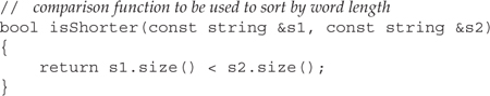
The first predicate we need will be used to sort the elements based on size. To do this sort, we need to define a predicate function that compares two strings and returns a bool indicating whether the first is shorter in length than the second:
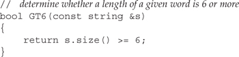
The other function we need will determine whether a given string is of length six or greater:
Although this function solves our problem, it is unnecessarily limited—the function hardwires the size into the function itself. If we wanted to find out how many words were of another length, we’d have to write another function. We could easily write a more general comparison function that took two parameters, the string and the size. However, the function we pass to count_if takes a single argument, so we cannot use the more general approach in this program. We’ll see a better way to write this part of our solution in Section 14.8.1 (p. 531).
Sorting Algorithms
The library defines four different sort algorithms, of which we’ve used the simplest, sort, tosort words into alphabetical order. In addition to sort, the library also defines a stable_sort algorithm. A stable_sort maintains the original order among equal elements. Ordinarily, we don’t care about the relative order of equal elements in a sorted sequence. After all, they’re equal. However, in this case, we have defined “equal” to mean “the same length.” Elements that have the same length can still be distinct when viewed alphabetically. By calling stable_sort, we maintain alphabetic order among those elements that have the same length.
Both sort and stable_sort are overloaded functions. One version uses the < operator for the element type to do the comparison. We used this version of sort to sort words before looking for duplicate elements. The second version takes a third parameter: the name of a predicate to use when comparing elements. That function must take two arguments of the same type as the element type and return a value that can be tested in a condition. We will use this second version, passing our isShorter function to compare elements:
// sort words by size, but maintain alphabetic order for words of the same size
stable_sort(words.begin(), words.end(), isShorter);
After this call, words is sorted by element size, but the words of each length are also still in alphabetical order:
![]()
Counting Words of Length Six or More
Now that we’ve reordered our vector by word size, our remaining problem is to count how many words are of length six or greater. The count_if algorithm handles this problem:
![]()
count_if executes by reading the range denoted by its first two parameters. It passes each value that it reads to the predicate function represented by its third argument. That function must take a single argument of the element type and must return a value that can be tested as a condition. The algorithm returns a count of the number of elements for which the function succeeded. In this case, count_if passes each word to GT6, which returns the bool value true if the word’s length is six or more.
Putting It All Together
Having looked at the program in detail, here is the program as a whole:
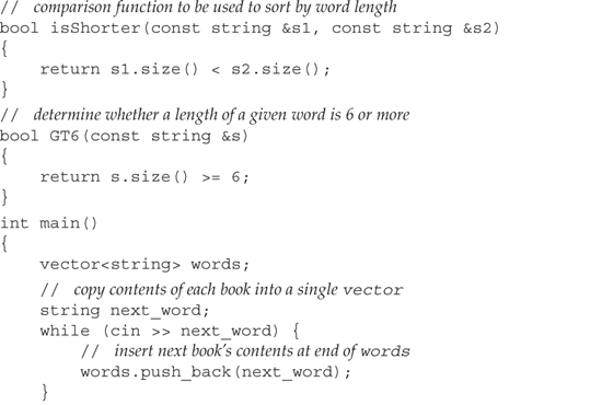
We leave as an exercise the problem of printing the words in size order.
11.3 Revisiting Iterators
In Section 11.2.2 (p. 398) we saw that the library defines iterators that are independent of a particular container. In fact, there are three additional kinds of iterators:
• insert iterators: These iterators are bound to a container and can be used to insert elements to the container.
• iostream iterators: These iterators can be bound to input or output streams and used to iterate through the associated IO stream.
• reverse iterators: These iterators move backward, rather than forward. Each container type defines its own reverse_iterator types, which are retuned by the rbegin and rend functions.
These iterator types are defined in the iterator header.
This section will look at each of these kinds of iterators and show how they can be used with the generic algorithms. We’ll also take a look at how and when to use the container const_iterators.
11.3.1 Insert Iterators
In Section 11.2.2 (p. 398) we saw that we can use back_inserter to create an iterator that adds elements to a container. The back_inserter function is an example of an inserter. An inserter is an iterator adaptor (Section 9.7, p. 348) that takes a container and yields an iterator that inserts elements into the specified container. When we assign through an insert iterator, the iterator inserts a new element. There are three kinds of inserters, which differ as to where elements are inserted:
• back_inserter, which creates an iterator that uses push_back.
• front_inserter, which uses push_front.
• inserter, which uses insert. In addition to a container, inserter takes a second argument: an iterator indicating the position ahead of which insertion should begin.
front_inserter Requires push_front
front_inserter operates similarly to back_inserter: It creates an iterator that treats assignment as a call to push_front on its underlying container.
We can use front_inserter only if the container has a push_front operation. Using front_inserter on a vector, or other container that does not have push_front, is an error.
inserter Yields an Iterator that Inserts at a Given Place
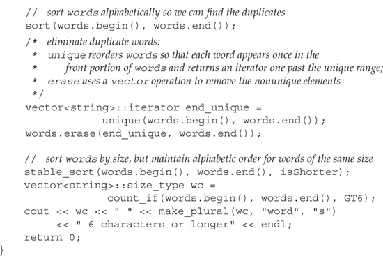
The inserter adaptor provides a more general form. This adaptor takes both a container and an iterator denoting a position at which to do the insertion:
We start by using find to locate an element in ilst. The call to replace_copy uses an inserter that will insert elements into ilst just before of the element denoted by the iterator returned from find. The effect of the call to replace_copy is to copy the elements from ivec, replacing each value of 100 by 0. The elements are inserted just ahead of the element denoted by it.
When we create an inserter, we say where to insert new elements. Elements are always inserted in front of the position denoted by the iterator argument to inserter.
We might think that we could simulate the effect of front_inserter by using inserter and the begin iterator for the container. However, an inserter behaves quite differently from front_inserter. When we use front_inserter, the elements are always inserted ahead of the then first element in the container. When we use inserter, elements are inserted ahead of a specific position. Even if that position initially is the first element, as soon as we insert an element in front of that element, it is no longer the one at the beginning of the container:

When we copy into ilst2, elements are always inserted ahead of any other element in the list. When we copy into ilst3, elements are inserted at a fixed point. That point started out as the head of the list, but as soon as even one element is added, it is no longer the first element.
Recalling the discussion in Section 9.3.3 (p. 318), it is important to understand that using front_inserter results in the elements appearing in the destination in reverse order.
11.3.2 iostream Iterators
Even though the iostream types are not containers, there are iterators that can be used with iostream objects: An istream_iterator reads an input stream, and an ostream_iterator writes an output stream. These iterators treat their corresponding stream as a sequence of elements of a specified type. Using a stream iterator, we can use the generic algorithms to read (or write) data to (or from) stream objects.
The stream iterators define only the most basic of the iterator operations: increment, dereference, and assignment. In addition, we can compare two istream iterators for equality (or inequality). There is no comparison for ostream iterators.
Defining Stream Iterators
The stream iterators are class templates: An istream_iterator can be defined for any type for which the input operator (the >> operator) is defined. Similarly, an ostream_iterator can be defined for any type that has an output operator (the << operator).
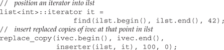
Table 11.1. iostream Iterator Constructors
When we create a stream iterator, we must specify the type of objects that the iterator will read or write:

We must bind an ostream_iterator to a specific stream. When we create an istream_iterator, we can bind it to a stream. Alternatively, we can supply no argument, which creates an iterator that we can use as the off-the-end value. There is no off-the-end iterator for ostream_iterator.
When we create an ostream_iterator, we may (optionally) provide a second argument that specifies a delimiter to use when writing elements to the output stream. The delimiter must be a C-style character string. Because it is a C-style string, it must be null-terminated; otherwise, the behavior is undefined.
Operations on istream_iterators
Constructing an istream_iterator bound to a stream positions the iterator so that the first dereference reads the first value from the stream.
Table 11.2. istream_iterator Operations
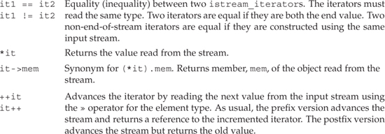
As an example, we could use an istream_iterator to read the standard input into a vector:
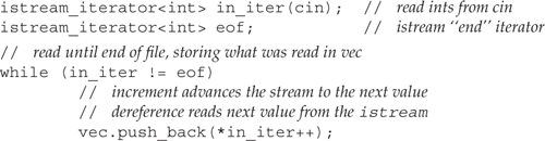
This loop reads ints from cin, and stores what was read in vec. On each trip the loop checks whether in_iter is the same as eof. That iterator was defined as the empty istream_iterator, which is used as the end iterator. An iterator bound to a stream is equal to the end iterator once its associated stream hits end-of-file or encounters another error.
The hardest part of this program is the argument to push_back, which uses the dereference and postfix increment operators. Precedence rules (Section 5.5, p. 163) say that the result of the increment is the operand to the dereference. Incrementing an istream_iterator advances the stream. However, the expression uses the postfix increment, which yields the old value of the iterator. The effect of the increment is to read the next value from the stream but return an iterator that refers to the previous value read. We dereference that iterator to obtain that value.
What is more interesting is that we could rewrite this program as:
![]()
Here we construct vec from a pair of iterators that denote a range of elements. Those iterators are istream_iterators, which means that the range is obtained by reading the associated stream. The effect of this constructor is to read cin until it hits end-of-file or encounters an input that is not an int. The elements that are read are used to construct vec.
Using ostream_iterators and istream_iterators
We can use an ostream_iterator to write a sequence of values to a stream in much the same way that we might use an iterator to assign a sequence of values to the elements of a container:
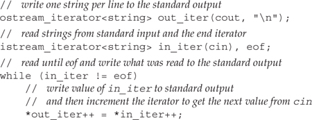
This program reads cin, writing each word it reads on separate line on cout.
We start by defining an ostream_iterator to write strings to cout, following each string by a newline. We define two istream_iterators that we’ll use to read strings from cin. The while loop works similarly to our previous example. This time, instead of storing the values we read into a vector, we print them to cout by assigning the values we read to out_iter.
The assignment works similarly to the one in the program on page 205 that copied one array into another. We dereference both iterators, assigning the right-hand value into the left, incrementing each iterator. The effect is to write what was read to cout and then increment each iterator, reading the next value from cin.
Using istream_iterators with Class Types
We can create an istream_iterator for any type for which an input operator (>>) exists. For example, we might use an istream_iterator to read a sequence of Sales_item objects to sum:

This program binds item_iter to cin and says that the iterator will read objects of type Sales_item. The program next reads the first record into sum:
sum = *item_iter++; // read first transaction into sum and get next record
This statement uses the dereference operator to fetch the first record from the standard input and assigns that value to sum. It increments the iterator, causing the stream to read the next record from the standard input.
The while loop executes until we hit end-of-file on cin. Inside the while, we compare the isbn of the record we just read with sum’s isbn. The first statement in the while uses the arrow operator to dereference the istream iterator and obtain the most recently read object. We then run the same_isbn member on that object and the object in sum.
If the isbns are the same, we increment the totals in sum. Otherwise, we print the current value of sum and reset it as a copy of the most recently read transaction. The last step in the loop is to increment the iterator, which in this case causes the next transaction to be read from the standard input. The loop continues until an error or end-of-file is encountered. Before exiting we remember to print the values associated with the last ISBN in the input.
Limitations on Stream Iterators
The stream iterators have several important limitations:
• It is not possible to read from an ostream_iterator, and it is not possible to write to an istream_iterator.
• Once we assign a value to an ostream_iterator, the write is committed. There is no way to subsequently change a value once it is assigned. Moreover, each distinct value of an ostream_iterator is expected to be used for output exactly once.
• There is no -> operator for ostream_iterator.
Using Stream Iterators with the Algorithms
As we know, the algorithms operate in terms of iterator operations. And as we’ve seen, stream iterators define at least some of the iterator operations. Because the stream iterators support iterator operations, we can use them with at least some of the generic algorithms. As an example, we could read numbers from the standard input and write the unique numbers we read on the standard output:

If the input to this program is
23 109 45 89 6 34 12 90 34 23 56 23 8 89 23
6 8 12 23 34 45 56 89 90 109
The program creates vec from the iterator pair, input and end_of_stream. The effect of this initializer is to read cin until end-of-file or an error occurs. The values read are stored in vec.
Once the input is read and vec initialized, we call sort to sort the input. Duplicated items from the input will be adjacent after the call to sort.
The program uses unique_copy, which is a copying version of unique. It copies the unique values in its input range to the destination iterator. This call uses our output iterator as the destination. The effect is to copy the unique values from vec to cout, following each value by a space.
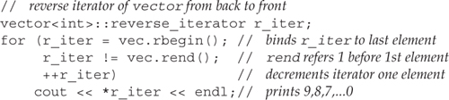
11.3.3 Reverse Iterators
A reverse iterator is an iterator that traverses a container backward. That is, it traverses from the last element toward the first. A reverse iterator inverts the meaning of increment (and decrement): ++ on a reverse iterator accesses the previous element; -- accesses the next element.
Recall that each container defines begin and end members. These members return respectively an iterator to the first element of the container and an iterator one past the last element of the container. The containers also define rbegin and rend, which return reverse iterators to the last element in the container and one “past” (that is, one before) the beginning of the container. As with ordinary iterators, there are both const and nonconst reverse iterators. Figure 11.1 on the facing page illustrates the relationship between these four iterators on a hypothetical vector named vec.
Figure 11.1. Comparing begin/end and rbegin/rend Iterators
Given a vector that contains the numbers from 0 to 9 in ascending order
![]()
the following for loop prints the elements in reverse order:
Although it may seem confusing to have the meaning of the increment and decrement operators reversed, doing so lets us use the algorithms transparently to process a container forward or backward. For example, we could sort our vector in descending order by passing sort a pair of reverse iterators:

Reverse Iterators Require Decrement Operators
Not surprisingly, we can define a reverse iterator only from an iterator that supports -- as well as ++. After all, the purpose of a reverse iterator is to move the iterator backward through the sequence. The iterators on the standard containers all support decrement as well as increment. However, the stream iterators do not, because it is not possible to move backward through a stream. Therefore, it is not possible to create a reverse iterator from a stream iterator.
Relationship between Reverse Iterators and Other Iterators
Suppose we have a string named line that contains a comma-separated list of words, and we want to print the first word in line. Using find, this task is easy:

If there is a comma in line, then comma refers to that comma; otherwise it is line.end(). When we print the string from line.begin() to comma we print characters up to the comma, or the entire string if there is no comma.
If we wanted the last word in the list, we could use reverse iterators instead:

Because we pass rbegin() and rend(), this call starts with the last character in line and searches backward. When find completes, if there is a comma, then rcomma refers to the last comma in the line—that is it refers to the first comma found in the backward search. If there is no comma, then rcomma is line.rend().
The interesting part comes when we try to print the word we found. The direct attempt
// wrong: will generate the word in reverse order
cout << string(line.rbegin(), rcomma) << endl;
generates bogus output. For example, had our input been
FIRST,MIDDLE,LAST
then this statement would print TSAL!
Figure 11.2 illustrates the problem: We are using reverse iterators, and such iterators process the string backward. To get the right output, we need to transform the reverse iterators line.rbegin() and rcomma into normal iterators that go forward. There is no need to transform line.rbegin() as we already know that the result of that transformation would be line.end(). We can transform rcomma by calling base, which is a member of each reverse iterator type:
Figure 11.2. Relationship between Reverse and Ordinary Iterators

// ok: get a forward iterator and read to end of line
cout << string(rcomma.base(), line.end()) << endl;
Given the same preceeding input, this statement prints LAST as expected.
The objects shown in Figure 11.2 visually illustrate the relationship between ordinary and reverse iterators. For example, rcomma and rcomma.base() refer to different elements, as do line.rbegin() and line.end(). These differences are needed to ensure that the range of elements whether processed forward or backward is the same. Technically speaking, the relationship between normal and reverse iterators is designed to accommodate the properties of a left-inclusive range (Section 9.2.1, p. 314), so that [line.rbegin(), rcomma) and [rcomma.base(), line.end()) refer to the same elements in line.
The fact that reverse iterators are intended to represent ranges and that these ranges are asymmetric has an important consequence. When we initialize or assign a reverse iterator from a plain iterator, the resulting iterator does not refer to the same element as the original.
11.3.4 const Iterators
Careful readers will have noted that in the program on page 392 that used find, we defined result as a const_iterator. We did so because we did not intend to use the iterator to change a container element.
On the other hand, we used a plain, nonconst iterator to hold the return from find_first_of on page 397, even though we did not intend to change any container elements in that program either. The difference in treatment is subtle and deserves an explanation.
The reason is that in the second case, we use the iterator as an argument to find_first_of:
![]()
The input range for this call is specified by it and the iterator returned from a call to roster1.end(). Algorithms require the iterators that denote a range to have exactly the same type. The iterator returned by roster1.end() depends on the type of roster1. If that container is a const object, then the iterator is const_iterator; otherwise, it is the plain iterator type. In this program, roster1 was not const, and so end returns an iterator.
If we defined it as a const_iterator, the call to find_first_of would not compile. The types of the iterators used to denote the range would not have been identical. it would have been a const_iterator, and the iterator returned by roster1.end() would be iterator.
11.3.5 The Five Iterator Categories
Iterators define a common set of operations, but some iterators are more powerful than other iterators. For example, ostream_iterators support only increment, dereference, and assignment. Iterators on vectors support these operations and the decrement, relational, and arithmetic operators as well. As a result, we can classify iterators based on the set of operations they provide.
Similarly, we can categorize algorithms by the kinds of operations they require from their iterators. Some, such as find, require only the ability to read through the iterator and to increment it. Others, such as sort, require the ability to read, write, and randomly access elements. The iterator operations required by the algorithms are grouped into five categories. These five categories correspond to five categories of iterators, which are summarized in Table 11.3.
Table 11.3. Iterator Categories
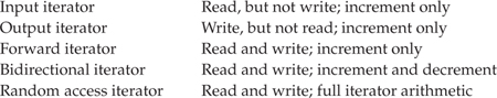
- Input iterators can read the elements of a container but are not guaranteed to be able to write into a container. An input iterator must provide the following minimum support:
• Equality and inequality operators (
==, !=) to compare two iterators.• Prefix and postfix increment (
++) to advance the iterator.• Dereference operator (
*) to read an element; dereference may appear only on the right-hand side of an assignment.• The arrow operator (
->) as a synonym for(*it).member—that is, dereference the iterator and fetch a member from the underlying object.Input iterators may be used only sequentially; there is no way to examine an element once the input iterator has been incremented. Generic algorithms requiring only this level of support include
findandaccumulate. The libraryistream_iteratortype is an input iterator. - Output iterators can be thought of as having complementary functionality to input iterators; An output iterator can be used to write an element but it is not guaranteed to support reading. Output iterators require:
• Prefix and postfix increment (
++) to advance the iterator.• Dereference (
*), which may appear only as the left-hand side of an assignment. Assigning to a dereferenced output iterator writes to the underlying element.Output iterators may require that each iterator value must be written exactly once. When using an output iterator, we should use
*once and only once on a given iterator value. Output iterators are generally used as a third argument to an algorithm and mark the position where writing should begin. For example, thecopyalgorithm takes an output iterator as its third parameter and copies elements from its input range to the destination indicated by the output iterator. Theostream_iteratortype is an output iterator. - Forward iterators read from and write to a given container. They move in only one direction through the sequence. Forward iterators support all the operations of both input iterators and output iterators. In addition, they can read or write the same element multiple times. We can copy a forward iterator to remember a place in the sequence so as to return to that place later. Generic algorithms that require a forward iterator include
replace. - Bidirectional iterators read from and write to a container in both directions. In addition to supporting all the operations of a forward iterator, a bidirectional iterator also supports the prefix and postfix decrement (
--) operators. Generic algorithms requiring a bidirectional iterator includereverse. All the library containers supply iterators that at a minimum meet the requirements for a bidirectional iterator. - Random-access iterators provide access to any position within the container in constant time. These iterators support all the functionality of bidirectional iterators. In addition, random-access iterators support:
• The relational operators
<, <=, >, and>=to compare the relative positions of two iterators.• Addition and subtraction operators
+, +=, -, and-=between an iterator and an integral value. The result is the iterator advanced (or retreated) the integral number of elements within the container.• The subtraction operator
-when applied to two iterators, which yields the distance between two iterators.• The subscript operator
iter[n]as a synonym for*(iter + n).Generic algorithms requiring a random-access iterator include the
sortalgorithms. Thevector, deque, andstringiterators are random-access iterators, as are pointers when used to access elements of a built-in array.
With the exception of output iterators, the iterator categories form a sort of hierarchy: Any iterator of a higher category can be used where an iterator of lesser power is required. We can call an algorithm requiring an input iterator with an input iterator or a forward, bidirectional, or random-access iterator. Only a random-access iterator may be passed to an algorithm requiring a random-access iterator.
The map, set, and list types provide bidirectional iterators. Iterators on string, vector, and deque are random-access iterators, as are pointers bound to arrays. An istream_iterator is an input iterator, and an ostream_iterator is an output iterator.
Key Concept: Associative Containers and the Algorithms
Although the map and set types provide bidirectional iterators, we can use only a subset of the algorithms on associative containers. The problem is that the key in an associative container is const. Hence, any algorithm that writes to elements in the sequence cannot be used on an associative container. We may use iterators bound to associative containers only to supply arguments that will be read.

The C++ standard specifies the minimum iterator category for each iterator parameter of the generic and numeric algorithms. For example, find—which implements a one-pass, read-only traversal over a container—minimally requires an input iterator. The replace function requires a pair of iterators that are at least forward iterators. The first two iterators to replace_copy must be at least forward. The third, which represents a destination, must be at least an output iterator.
For each parameter, the iterator must be at least as powerful as the stipulated minimum. Passing an iterator of a lesser power results in an error; passing an stronger iterator type is okay.
Errors in passing an invalid category of iterator to an algorithm are not guaranteed to be caught at compile-time.
Exercises Section 11.3.5
Exercise 11.23: List the five iterator categories and the operations that each supports.
Exercise 11.24: What kind of iterator does a list have? What about a vector?
Exercise 11.25: What kinds of iterators do you think copy requires? What about reverse or unique?
Exercise 11.26: Explain why each of the following is incorrect. Identify which errors should be caught during compilation.

11.4 Structure of Generic Algorithms
Just as there is a consistent design pattern behind the containers, there is a common design underlying the algorithms. Understanding the design behind the library makes it easier to learn and easier to use the algorithms. Because there are more than 100 algorithms, it is much better to understand their structure than to memorize the whole list of algorithms.
The most fundamental property of any algorithm is the kind(s) of iterators it expects. Each algorithm specifies for each of its iterator parameters what kind of iterator can be supplied. If a parameter must be a random-access iterator, then we can provide an iterator for a vector or a deque, or we can supply a pointer into an array. Iterators on the other containers cannot be used with such algorithms.
A second way is to classify the algorithms is as we did in the beginning of this chapter. We can categorize them by what actions they take on the elements:
• Some are read-only and leave element values and ordering unchanged.
• Others assign new values to specific elements.
• Others move values from one element to another.
As we’ll see in the remainder of this section, there are two additional patterns to the algorithms: One pattern is defined by the parameters the algorithms take; the other is defined by two function naming and overloading conventions.
11.4.1 Algorithm Parameter Patterns
Superimposed on any other classification of the algorithms is a set of parameter conventions. Understanding these parameter conventions can aid in learning new algorithms—by knowing what the parameters mean, you can concentrate on understanding the operation the algorithm performs. Most of algorithms take one of the following four forms:
alg (beg, end, other parms);
alg (beg, end, dest, other parms);
alg (beg, end, beg2, other parms);
alg (beg, end, beg2, end2, other parms);
where alg is the name of the algorithm, and beg and end denote the range of elements on which the algorithm operates. We typically refer to this range as the “input range” of the algorithm. Although nearly all algorithms take an input range, the presence of the other parameters depends on the work being performed. The common ones listed here—dest, beg2 and end2—are all iterators. When used, these iterators fill similar roles. In addition to these iterator parameters, some algorithms take additional, noniterator parameters that are algorithm-specific.
Algorithms with a Single Destination Iterator
A dest parameter is an iterator that denotes a destination used to hold the output. Algorithms assume that it is safe to write as many elements as needed.
When calling these algorithms, it is essential to ensure that the output container is sufficiently large to hold the output, which is why they are frequently called with insert iterators or ostream_iterators. If we call these algorithms with a container iterator, the algorithm assumes there are as many elements as needed in that container.
If dest is an iterator on a container, then the algorithm writes its output to existing elements within the container. More commonly, dest is bound to an insert iterator (Section 11.3.1, p. 406) or an ostream_iterator. An insert iterator adds elements to the container, ensuring that there is enough space. An ostream_iterator writes to an output stream, again presenting no problem regardless of how many elements are written.
Algorithms with a Second Input Sequence
Algorithms that take either beg2 alone or beg2 and end2 use these iterators to denote a second input range. These algorithms typically use the elements from the second range in combination with the input range to perform a computation. When an algorithm takes both beg2 and end2, these iterators are used to denote the entire second range. That is, the algorithm takes two completely specified ranges: the input range denoted by beg and end, and a second input range denoted by beg2 and end2.
Algorithms that take beg2 but not end2 treat beg2 as the first element in the second input range. The end of this range is not specified. Instead, these algorithms assume that the range starting at beg2 is at least as large as the one denoted by beg, end.
As with algorithms that write to dest, algorithms that take beg2 alone assume that the sequence beginning at beg2 is as large as the range denoted by beg and end.
11.4.2 Algorithm Naming Conventions
The library uses a set of consistent naming and overload conventions that can simplify learning the library. There are two important patterns. The first involves algorithms that test the elements in the input range, and the second applies to those that reorder elements within the input range.
Distinguishing Versions that Take a Value or a Predicate
Many algorithms operate by testing elements in their input range. These algorithms typically use one of the standard relational operators, either == or <. Most of the algorithms provide a second version that allows the programmer to override the use of the operator and instead to supply a comparison or test function.
Algorithms that reorder the container elements use the < operator. These algorithms define a second, overloaded version that takes an additional parameter representing a different operation to use to order the elements:
![]()
Algorithms that test for a specific value use the == operator by default. These algorithms provide a second named—not overloaded—version with a parameter that is a predicate (Section 11.2.3, p. 402). Algorithms that take a predicate have the suffix _if appended:
![]()
These algorithms both find the first instance of a specific element in the input range. The find algorithm looks for a specific value; the find_if algorithm looks for a value for which pred returns a nonzero value.
The reason these algorithms provide a named version rather than an over-loaded one is that both versions take the same number of parameters. In the case of the ordering algorithms, it is easy to disambiguate a call based solely on the number of parameters. In the case of algorithms that look for a specific element, the number of parameters is the same whether testing for a value or testing a predicate. Overloading ambiguities (Section 7.8.2, p. 269) would therefore be possible, albeit rare, and so the library provides two named versions for these algorithms rather than relying on overloading.
Distinguishing Versions that Copy from Those that Do Not
Independently of whether an algorithm tests its elements, the algorithm may re-arrange elements within the input range. By default, such algorithms write the rearranged elements back into their input range. These algorithms also provide a second, named version that writes to a specified output destination. These algorithms append _copy to their names:
reverse(beg, end);
reverse_copy(beg, end, dest);
The reverse function does what its name implies: It reverses the order of the elements in the input sequence. The first version reverses the elements in the input sequence itself. The second version, reverse_copy, makes a copy of the elements, placing them in reverse order in the sequence that begins at dest.
11.5 Container-Specific Algorithms
The iterators on list are bidirectional, not random access. Because the list container does not support random access, we cannot use the algorithms that require random-access iterators. These algorithms include the sort-related algorithms. There are other algorithms, defined generically, such as merge, remove, reverse, and unique, that can be used on lists but at a cost in performance. These algorithms can be implemented more efficiently if they can take advantage of how lists are implemented.
Exercises Section 11.4.2
Exercise 11.27: The library defines the following algorithms:

Based only on the names and parameters to these functions, describe the operation that these algorithms perform.
Exercise 11.28: Assume lst is a container that holds 100 elements. Explain the following program fragment and fix any bugs you think are present.
vector<int> vec1;
reverse_copy(lst.begin(), lst.end(), vec1.begin());
It is possible to write much faster algorithms if the internal structure of the list can be exploited. Rather than relying solely on generic operations, the library defines a more elaborate set of operations for list than are supported for the other sequential containers. These list-specific operations are described in Table 11.4 on the next page. Generic algorithms not listed in the table that take bidirectional or weaker iterators execute equally efficiently on lists as on other containers.
Table 11.4. list-Specific Operations
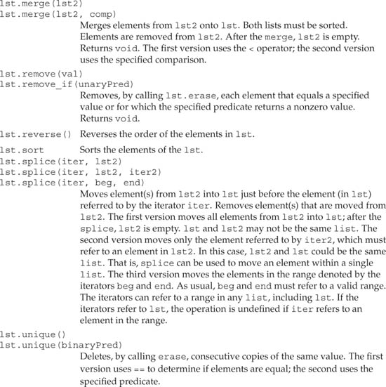

The list member versions should be used in preference to the generic algorithms when applied to a list object.
Most of the list-specific algorithms are similar—but not identical—to their counterparts that we have already seen in their generic forms:
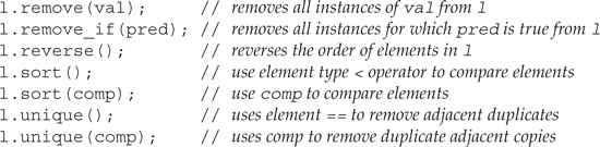
There are two crucially important differences between the list-specific operations and their generic counterparts. One difference is that the list versions of remove and unique change the underlying container; the indicated elements are actually removed. For example, second and subsequent duplicate elements are removed from the list by list::unique.
Unlike the corresponding generic algorithms, the list-specific operations do add and remove elements.
The other difference is that the list operations, merge and splice, are destructive on their arguments. When we use the generic version of merge, the merged sequence is written to a destination iterator, and the two input sequences are left unchanged. In the case of the merge function that is a member of list, the argument list is destroyed—elements are moved from the argument and removed as they are merged into the list object on which merge was called.
Chapter Summary
One of the more important contributions from the standardization process for C++ was the creation and expansion of the standard library. The containers and algorithms libraries are a cornerstone of the standard library. The library defines more than 100 algorithms. Fortunately, the algorithms have a consistent architecture, which makes learning and using them easier.
The algorithms are type independent: They generally operate on a sequence of elements that can be stored in a library container type, a built-in array, or even a generated sequence, such as by reading or writing to a stream. Algorithms achieve their type independence by operating in terms of iterators. Most algorithms take a pair of iterators denoting a range of elements as the first two arguments. Additional iterator arguments might include an output iterator denoting a destination, or another iterator or iterator pair denoting a second input sequence.
Iterators can be categorized by the operations that they support. There are five iterator categories: input, output, forward, bidirectional, and random access. An iterator belongs to a particular category if it supports the operations required for that iterator category.
Just as iterators are categorized by their operations, iterator parameters to the algorithms are categorized by the iterator operations they require. Algorithms that only read their sequences often require only input iterator operations. Those that write to a destination iterator often require only the actions of an output iterator, and so on.
Algorithms that look for a value often have a second version that looks for an element for which a predicate returns a nonzero value. For such algorithms, the name of the second version has the suffix _if. Similarly, many algorithms provide so-called copying versions. These write the (transformed) elements to an output sequence rather than writing back into the input range. Such versions have names that end with _copy.
A third pattern is whether algorithms read, write, or reorder elements. Algorithms never directly change the size of the sequences on which they operate. (If an argument is an insert iterator, then that iterator might add elements, but the algorithm does not do so directly.) They may copy elements from one position to another but cannot directly add or remove elements.
Defined Terms
Iterator adaptor that takes a reference to a container and generates an insert iterator that uses push_back to add elements to the specified container.
Same operations as forward iterators plus the ability to use to move backward through the sequence.
Iterator that can read and write elements, but does not support --.
Iterator adaptor that given a container, generates an insert iterator that uses push_front to add elements to the beginning of that container.
Type-independent algorithms.
Iterator that can read but not write elements.
Iterator that uses a container operation to insert elements rather than overwrite them. When a value is assigned to an insert iterator, the effect is to insert the element with that value into the sequence.
Iterator adaptor that takes an iterator and a reference to a container and generates an insert iterator that uses insert to add elements just ahead of the element referred to by the given iterator.
Stream iterator that reads an input stream.
Conceptual organization of iterators based on the operations that an iterator supports. Iterator categories form a hierarchy, in which the more powerful categories offer the same operations as the lesser categories. The algorithms use iterator categories to specify what operations the iterator arguments must support. As long as the iterator provides at least that level of operation, it can be used. For Example, some algorithms require only input iterators. Such algorithms can be called on any iterator other than one that meets only the output iterator requirements. Algorithms that require random-access iterators can be used only on iterators that support random-access operations.
An iterator that marks the end of a range of elements in a sequence. The off-the-end iterator is used as a sentinel and refers to an element one past the last element in the range. The off-the-end iterator may refer to a nonexistent element, so it must never be dereferenced.
Iterator that writes to an output stream.
Iterator that can write but not read elements.
Function that returns a type that can be converted to bool. Often used by the generic algorithms to test elements. Predicates used by the library are either unary (taking one argument) or binary (taking two).
Same operations as bidirectional iterators plus the ability to use the relational operators to compare iterator values and the ability to do arithmetic on iterators, thus supporting random access to elements.
Iterator that moves backward through a sequence. These iterators invert the meaning of ++ and --.
Iterator that can be bound to a stream.