Appendix A. The Library
CONTENTS
Section A.1 Library Names and Headers 810
Section A.2 A Brief Tour of the Algorithms 811
Section A.3 The IO Library Revisited 825
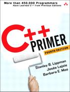
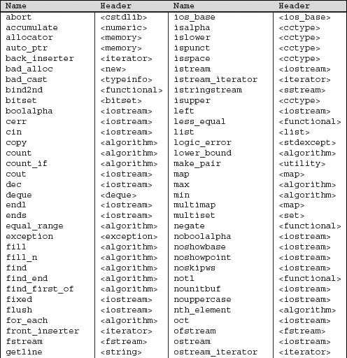
This appendix presents additional useful details about the library. We’ll start by collecting in one place the names we used from the standard library. Table A.1 on the next page lists each name and the header that defines that name.
Chapter 11 covered the library algorithms. That chapter illustrated how some of the more common algorithms are used, and described the architecture that underlies the algorithms library. In this Appendix, we list all the algorithms, organized by the kinds of operations they perform.
We close by examining some additional IO library capabilities: format control, unformatted IO, and random access on files. Each IO type defines a collection of format states and associated functions to control those states. These format states give us finer control over how input and output works. The IO we’ve done has all been formatted—the input and output routines know about the types we use and format the data on input or output accordingly. There are also unformatted IO functions that deal with the stream at the char level, doing no interpretation of the data. In Chapter 8 we saw that the fstream type can read and write the same file. In this Appendix, we’ll see how to do so.
A.1 Library Names and Headers
Our programs mostly did not show the actual #include directives needed to compile the program. As a convenience to our readers, Table A.1 lists the library names our programs used and the header in which they may be found.
Table A.1. Standard Library Names and Headers
A.2 A Brief Tour of the Algorithms
Chapter 11 introduced the generic algorithms and outlined their underlying architecture. The library defines more than 100 algorithms. Learning to use them requires understanding their structure rather than memorizing the details of each algorithm. In this section we describe each of the algorithms. In it, we organize the algorithms by the type of action the algorithm performs.
A.2.1 Algorithms to Find an Object
The find and count algorithms search the input range for a specific value. find returns an iterator to an element; count returns the number of matching elements.
Simple Find Algorithms
These algorithms require input iterators. The find and count algorithms look for specific elements. The find algorithms return an iterator referring to the first matching element. The count algorithms return a count of how many times the element occurs in the input sequence.
find(beg, end, val)
count(beg, end, val)
Looks for element(s) in input range equal to val. Uses the equality (==) operator of the underlying type. find returns an iterator to the first matching element or end if no such element exists. count returns a count of how many times val occurs.
find_if(beg, end, unaryPred)
count_if(beg, end, unaryPred)
Looks for element(s) in input range for which unaryPred is true. The predicate must take a single parameter of the value_type of the input range and return a type that can be used as a condition.
find returns an iterator to first element for which unaryPred is true, or end if no such element exists. count applies unaryPred to each element and returns the number of elements for which unaryPred was true.
Algorithms to Find One of Many Values
These algorithms require two pairs of forward iterators. They search for the first (or last) element in the first range that is equal to any element in the second range. The types of beg1 and end1 must match exactly, as must the types of beg2 and end2.
There is no requirement that the types of beg1 and beg2 match exactly. However, it must be possible to compare the element types of the two sequences. So, for example, if the first sequence is a list<string>, then the second could be a vector<char*>.
Each algorithm is overloaded. By default, elements are tested using the == operator for the element type. Alternatively, we can specify a predicate that takes two parameters and returns a bool indicating whether the test between these two elements succeeds or fails.
find_first_of(beg1, end1, beg2, end2)
Returns an iterator to the first occurrence in the first range of any element from the second range. Returns end1 if no match found.
find_first_of(beg1, end1, beg2, end2, binaryPred)
Uses binaryPred to compare elements from each sequence. Returns an iterator to the first element in the first range for which the binaryPred is true when applied to that element and an element from the second sequence. Returns end1 if no such element exits.
find_end(beg1, end1, beg2, end2)
find_end(beg1, end1, beg2, end2, binaryPred)
Operates like find_first_of, except that it searches for the last occurrence of any element from the second sequence.
As an example, if the first sequence is 0,1,1,2,2,4,0,1 and the second sequence is 1,3,5,7,9, then find_end would return an iterator denoting the last element in the input range, and find_first_of would return an iterator to the second element—in this example, it returns the first 1 in the input sequence.
Algorithms to Find a Subsequence
These algorithms require forward iterators. They look for a subsequence rather than a single element. If the subsequence is found, an iterator is returned to the first element in the subsequence. If no subsequence is found, the end iterator from the input range is returned.
Each function is overloaded. By default, the equality (==) operator is used to compare elements; the second version allows the programmer to supply a predicate to test instead.
adjacent_find(beg, end)
adjacent_find(beg, end, binaryPred)
Returns an iterator to the first adjacent pair of duplicate elements. Returns end if there are no adjacent duplicate elements. In the first case, duplicates are found by using ==. In the second, duplicates are those for which the binaryPred is true.
search(beg1, end1, beg2, end2)
search(beg1, end1, beg2, end2, binaryPred)
Returns an iterator to the first position in the input range at which the second range occurs as a subsequence. Returns end1 if the subsequence is not found. The types of beg1 and beg2 may differ but must be compatible: It must be possible to compare elements in the two sequences.
search_n(beg, end, count, val)
search_n(beg, end, count, val, binaryPred)
Returns an iterator to the beginning of a subsequence of count equal elements. Returns end if no such subsequence exists. The first version looks for count occurrences of the given value; the second version count occurrences for which the binaryPred is true.
A.2.2 Other Read-Only Algorithms
These algorithms require input iterators for their first two arguments. The equal and mismatch algorithms also take an additional input iterator that denotes a second range. There must be at least as many elements in the second sequence as there are in the first. If there are more elements in the second, they are ignored. If there are fewer, it is an error and results in undefined run-time behavior.
As usual, the types of the iterators denoting the input range must match exactly. The type of beg2 must be compatible with the type of beg1. That is, it must be possible to compare elements in both sequences.
The equal and mismatch functions are overloaded: One version uses the element equality operator (==) to test pairs of elements; the other uses a predicate.
for_each(beg, end, f)
Applies the function (or function object (Section 14.8, p. 530)) f to each element in its input range. The return value, if any, from f is ignored. The iterators are input iterators, so the elements may not be written by f. Typically, for_each is used with a function that has side effects. For example, f might print the values in the range.
mismatch(beg1, end1, beg2)
mismatch(beg1, end1, beg2, binaryPred)
Compares the elements in two sequences. Returns a pair of iterators denoting the first elements that do not match. If all the elements match, then the pair returned is end1, and an iterator into beg2 offset by the size of the first sequence.
equal(beg1, end1, beg2)
equal(beg1, end1, beg2, binaryPred)
Determines whether two sequences are equal. Returns true if each element in the input range equals the corresponding element in the sequence that begins at beg2.
For example, given the sequences meet and meat, a call to mismatch would return a pair containing iterators referring to the second e in the first sequence and to the element a in the second sequence. If, instead, the second sequence were meeting, and we called equal, then the pair returned would be end1 and an iterator denoting the element i in the second range.
A.2.3 Binary-Search Algorithms
Although these algorithms may be used with forward iterators, they offer specialized versions that are much faster when used with random-access iterators.
These algorithms perform a binary search, which means that the input sequence must be sorted. These algorithms behave similarly to the associative container members of the same name (Section 10.5.2, p. 377). The equal_range, lower_bound, and upper_bound algorithms return an iterator that refers to the positions in the container at which the given element could be inserted while still preserving the container’s ordering. If the element is larger than any other in the container, then the iterator that is returned might be the off-the-end iterator.
Each algorithm provides two versions: The first uses the element type’s less-than operator (<) to test elements; the second uses the specified comparison.
lower_bound(beg, end, val)
lower_bound(beg, end, val, comp)
Returns an iterator to the first position in which val can be inserted while preserving the ordering.
upper_bound(beg, end, val)
upper_bound(beg, end, val, comp)
Returns an iterator to the last position in which val can be inserted while preserving the ordering.
equal_range(beg, end, val)
equal_range(beg, end, val, comp)
Returns an iterator pair indicating the subrange in which val could be inserted while preserving the ordering.
binary_search(beg, end, val)
binary_search(beg, end, val, comp)
Returns a bool indicating whether the sequence contains an element that is equal to val. Two values x and y are considered equal if x < y and y <x both yield false.
A.2.4 Algorithms that Write Container Elements
Many algorithms write container elements. These algorithms can be distinguished both by the kinds of iterators on which they operate and by whether they write elements in the input range or write to a specified destination.
The simplest algorithms read elements in sequence, requiring only input iterators. Those that write back to the input sequence require forward iterators. Some read the sequence backward, thus requiring bidirectional iterators. Algorithms that write to a separate destination, as usual, assume the destination is large enough to hold the output.
Algorithms that Write but do Not Read Elements
These algorithms require an output iterator that denotes a destination. They take a second argument that specifies a count and write that number of elements to the destination.
fill_n(dest, cnt, val)
generate_n(dest, cnt, Gen)
Write cnt values to dest. The fill_n function writes cnt copies of the value val; generate_n evaluates the generator Gen() cnt times. A generator is a function (or function object (Section 14.8, p. 530)) that is expected to produce a different return value each time it is called.
Algorithms that Write Elements Using Input Iterators
Each of these operations reads an input sequence and writes to an output sequence denoted by dest. They require dest to be an output iterator, and the iterators denoting the input range must be input iterators. The caller is responsible for ensuring that dest can hold as many elements as necessary given the input sequence. These algorithms return dest incremented to denote one past the last element written.
copy(beg, end, dest)
Copies the input range to the sequence beginning at iterator dest.
transform(beg, end, dest, unaryOp)
transform(beg, end, beg2, dest, binaryOp)
Applies the specified operation to each element in the input range, writing the result to dest. The first version applies a unary operation to each element in the input range. The second applies a binary operation to pairs of elements. It takes the first argument to the binary operation from the sequence denoted by beg and end and takes the second argument from the sequence beginning at beg2. The programmer must ensure that the sequence beginning at beg2 has at least as many elements as are in the first sequence.
replace_copy(beg, end, dest, old_val, new_val)
replace_copy_if(beg, end, dest, unaryPred, new_val)
Copies each element to dest, replacing specified elements by the new_val. The first version replaces those elements that are == to old_val. The second version replaces those elements for which unaryPred is true.
merge(beg1, end1, beg2, end2, dest)
merge(beg1, end1, beg2, end2, dest, comp)
Both input sequences must be sorted. Writes a merged sequence to dest. The first version compares elements using the < operator; the second version uses the given comparison.
Algorithms that Write Elements Using Forward Iterators
These algorithms require forward iterators because they write elements in their input sequence.
swap(elem1, elem2)
iter_swap(iter1, iter2)
Parameters to these functions are references, so the arguments must be writable. Swaps the specified element or elements denoted by the given iterators.
swap_ranges(beg1, end1, beg2)
Swaps the elements in the input range with those in the second sequence beginning at beg2. The ranges must not overlap. The programmer must ensure that the sequence starting at beg2 is at least as large as the input sequence. Returns beg2 incremented to denote the element just after the last one swapped.
fill(beg, end, val)
generate(beg, end, Gen)
Assigns a new value to each element in the input sequence. fill assigns the value val; generate executes Gen() to create new values.
replace(beg, end, old_val, new_val)
replace_if(beg, end, unaryPred, new_val)
Replace each matching element by new_val. The first version uses == to compare elements with old_val; the second version executes unaryPred on each element, replacing those for which unaryPred is true.
Algorithms that Write Elements Using Bidirectional Iterators
These algorithms require the ability to go backward in the sequence, and so they require bidirectional iterators.
copy_backward(beg, end, dest)
Copies elements in reverse order to the output iterator dest. Returns dest incremented to denote one past the last element copied.
inplace_merge(beg, mid, end)
inplace_merge(beg, mid, end, comp)
Merges two adjacent subsequences from the same sequence into a single, ordered sequence: The subsequences from beg to mid and from mid to end are merged into beg to end. First version uses < to compare elements; second version uses a specified comparison. Returns void.
A.2.5 Partitioning and Sorting Algorithms
The sorting and partitioning algorithms provide various strategies for ordering the elements of a container.
A partition divides elements in the input range into two groups. The first group consists of those elements that satisfy the specified predicate; the second, those that do not. For example, we can partition elements in a container based on whether the elements are odd, or on whether a word begins with a capital letter, and so forth.
Each of the sorting and partitioning algorithms provides stable and unstable versions. A stable algorithm maintains the relative order of equal elements. For example, given the sequence
{ "pshew", "Honey", "tigger", "Pooh" }
a stable partition based on whether a word begins with a capital letter generates the sequence in which the relative order of the two word categories is maintained:
{ "Honey", "Pooh", "pshew", "tigger" }
The stable algorithms do more work and so may run more slowly and use more memory than the unstable counterparts.
Partitioning Algorithms
These algorithms require bidirectional iterators.
stable_partition(beg, end, unaryPred)
partition(beg, end, unaryPred)
Uses unaryPred to partition the input sequence. Elements for which unaryPred is true are put at the beginning of the sequence; those for which the predicate is false are at the end. Returns an iterator just past the last element for which unaryPred is true.
Sorting Algorithms
These algorithms require random-access iterators. Each of the sorting algorithms provides two overloaded versions. One version uses element operator < to compare elements; the other takes an extra parameter that specifies the comparison. These algorithms require random-access iterators. With one exception, these algorithms return void; partial_sort_copy returns an itertor into the destination.
The partial_sort and nth_element algorithms do only part of the job of sorting the sequence. They are often used to solve problems that might otherwise be handled by sorting the entire sequence. Because these operations do less work, they typically are faster than sorting the entire input range.
sort(beg, end)
stable_sort(beg, end)
sort(beg, end, comp)
stable_sort(beg, end, comp)
Sorts the entire range.
partial_sort(beg, mid, end)
partial_sort(beg, mid, end, comp)
Sorts a number of elements equal to mid – beg. That is, if mid – beg is equal to 42, then this function puts the lowest-valued elements in sorted order in the first 42 positions in the sequence. After partial_sort completes, the elements in the range from beg up to but not including mid are sorted. No element in the sorted range is larger than any element in the range after mid. The order among the unsorted elements is unspecified.
As an example, we might have a collection of race scores and want to know what the first-, second- and third-place scores are but don’t care about the order of the other times. We might sort such a sequence as follows:
![]()
partial_sort_copy(beg, end, destBeg, destEnd)
partial_sort_copy(beg, end, destBeg, destEnd, comp)
Sorts elements from the input range and puts as much of the sorted sequence as fits into the sequence denoted by the iterators destBeg and destEnd. If the destination range is the same size or has more elements than the input range, then the entire input range is sorted and stored starting at destBeg. If the destination size is smaller, then only as many sorted elements as will fit are copied.
Returns an iterator into the destination that refers just after the last element that was sorted. The returned iterator will be destEnd if that destination sequence is smaller or equal in size to the input range.
nth_element(beg, nth, end)
nth_element(beg, nth, end, comp)
The argument nth must be an iterator positioned on an element in the input sequence. After nth_element, the element denoted by that iterator has the value that would be there if the entire sequence were sorted. The elements in the container are also partitioned around nth: Those before nth are all smaller than or equal to the value denoted by nth, and the ones after it are greater than or equal to it. We might use nth_element to find the value closest to the median:
![]()
A.2.6 General Reordering Operations
Several algorithms reorder the elements in a specified way. The first two, remove and unique, reorder the container so that the elements in the first part of the sequence meet some criteria. They return an iterator marking the end of this subsequence. Others, such as reverse, rotate, and random_shuffle rearrange the entire sequence.
These algorithms operate “in place;” they rearrange the elements in the input sequence itself. Three of the reordering algorithms offer “copying” versions. These algorithms, remove_copy, rotate_copy, and unique_copy, write the reordered sequence to a destination rather than rearranging elements directly.
Reordering Algorithms Using Forward Iterators
These algorithms reorder the input sequence. They require that the iterators be at least forward iterators.
remove(beg, end, val)
remove_if(beg, end, unaryPred)
“Removes” elements from the sequence by overwriting them with elements that are to be kept. The removed elements are those that are == to val or for which unaryPred is true. Returns an iterator just past the last element that was not removed.
For example, if the input sequence is hello world and val is o, then a call to remove will overwrite the two elements that are the letter 'o' by shifting the sequence to the left twice. The new sequence will be hell wrldld. The returned iterator will denote the element after the first d.
unique(beg, end)
unique(beg, end, binaryPred)
“Removes” all but the first of each consecutive group of matching elements. Returns an iterator just past the last unique element. First version uses == to determine whether two elements are the same; second version uses the predicate to test adjacent elements.
For example, if the input sequence is boohiss, then after the call to unique, the first sequence will contain bohisss. The iterator returned will point to the element after the first s. The value of the remaining two elements in the sequence is unspecified.
rotate(beg, mid, end)
Rotates the elements around the element denoted by mid. The element at mid becomes the first element; those from mid + 1 through end come next, followed by the range from beg to mid. Returns void.
For example, given the input sequence hissboo, if mid denotes the character b, then rotate would reorder the sequence as boohiss.
Reordering Algorithms Using Bidirectional Iterators
Because these algorithms process the input sequence backward, they requre bidirectional iterators.
reverse(beg, end)
reverse_copy(beg, end, dest)
Reverses the elements in the sequence. reverse operates in place; it writes the rearranged elements back into the input sequence. reverse_copy copies the elements in reverse order to the output iterator dest. As usual, the programmer must ensure that dest can be used safely. reverse returns void; reverse_copy returns an iterator just past the last element copied into the destination.
Reordering Algorithms Writing to Output Iterators
These algorithms require forward iterators for the input sequence and an output iterator for the destination.
Each of the preceding general reordering algorithms has an _copy version. These _copy versions perform the same reordering but write the reordered elements to a specified destination sequence rather than changing the input sequence. Except for rotate_copy, which requires forward iterators, the input range is specified by input iterators. The dest iterator must be an output iterator and, as usual, the programmer must guarantee that the destination can be written safely. The algorithms return the dest iterator incremented to denote one past the last element copied.
remove_copy(beg, end, dest, val)
remove_copy_if(beg, end, dest, unaryPred)
Copies elements except those matching val or for which unaryPred return true into dest.
unique_copy(beg, end, dest)
unique_copy(beg, end, dest, binaryPred)
Copies unique elements to dest.
rotate_copy(beg, mid, end, dest)
Like rotate except that it leaves its input sequence unchanged and writes the rotated sequence to dest. Returns void.
Reordering Algorithms Using Random-Access Iterators
Because these algorithms rearrange the elements in a random order, they require random-access iterators.
random_shuffle(beg, end)
random_shuffle(beg, end, rand)
Shuffles the elements in the input sequence. The second version takes a random-number generator. That function must take and return a value of the iterator’s difference_type. Both versions return void.
A.2.7 Permutation Algorithms
Consider the following sequence of three characters: abc. There are six possible permutations on this sequence: abc, acb, bac, bca, cab, and cba. These permutations are listed in lexicographical order based on the less-than operator. That is, abc is the first permutation because its first element is less than or equal to the first element in every other permutation, and its second element is smaller than any permutation sharing the same first element. Similarly, acb is the next permutation because it begins with a, which is smaller than the first element in any remaining permutation. Those permutations that begin with b come before those that begin with c.
For any given permutation, we can say which permutation comes before it and which after it. Given the permutation bca, we can say that its previous permutation is bac and that its next permutation is cab. There is no previous permutation of the sequence abc, nor is there a next permutation of cba.
The library provides two permutation algorithms that generate the permutations of a sequence in lexicographical order. These algorithms reorder the sequence to hold the (lexicographically) next or previous permutation of the given sequence. They return a bool that indicates whether there was a next or previous permutation.
The algorithms each have two versions: One uses the element type < operator, and the other takes an extra argument that specifies a comparison to use to compare the elements. These algorithms assume that the elements in the sequence are unique. That is, the algorithms assume that no two elements in the sequence have the same value.
Permutation Algorithms Require Bidirectional Iterators
To produce the permutation, the sequence must be processed both forward and backward, thus requiring bidirectional iterators.
next_permutation(beg, end)
next_permutation(beg, end, comp)
If the sequence is already in the last permutation, then next_permutation reorders the sequence to be the lowest permutation and returns false. Otherwise, it transforms the input sequence into the next permutation, which is the lexicographically next ordered sequence and returns true. The first version uses the element < operator to compare elements; the second version uses specified comparison.
prev_permutation(beg, end)
prev_permutation(beg, end, comp)
Like next_permutation, but transforms the sequence to form the previous permutation. If this is the smallest permutation, then it reorders the sequence to be the largest permutation and returns false.
A.2.8 Set Algorithms for Sorted Sequences
The set algorithms implement general set operations on a sequence that is in sorted order.

These algorithms are distinct from the library set container and should not be confused with operations on sets. Instead, these algorithms provide setlike behavior on an ordinary sequential container (vector, list, etc.) or other sequence, such as an input stream.
With the exception of includes, they also take an output iterator. As usual, the programmer must ensure that the destination is large enough to hold the generated sequence. These algorithms return their dest iterator incremented to denote the element just after the last one that was written to dest.
Each algorithm provides two forms: The first uses the < operator for the element type to compare elements in the two input sequences. The second takes a comparison, which is used to compare the elements.
Set Algorithms Require Input Iterators
These algorithms process elements sequentially, requiring input iterators.
includes(beg, end, beg2, end2)
includes(beg, end, beg2, end2, comp)
Returns true if every element in the second sequence is contained in the input sequence. Returns false otherwise.
set_union(beg, end, beg2, end2, dest)
set_union(beg, end, beg2, end2, dest, comp)
Creates a sorted sequence of the elements that are in either sequence. Elements that are in both sequences occur in the output sequence only once. Stores the sequence in dest.
set_intersection(beg, end, beg2, end2, dest)
set_intersection(beg, end, beg2, end2, dest, comp)
Creates a sorted sequence of elements present in both sequences. Stores the sequence in dest.
set_difference(beg, end, beg2, end2, dest)
set_difference(beg, end, beg2, end2, dest, comp)
Creates a sorted sequence of elements present in the first container but not in the second.
set_symmetric_difference(beg, end, beg2, end2, dest)
set_symmetric_difference(beg, end, beg2, end2, dest, comp)
Creates a sorted sequence of elements present in either container but not in both.
A.2.9 Minimum and Maximum Values
The first group of these algorithms are unique in the library in that they operate on values rather than sequences. The second set takes a sequence that is denoted by input iterators.
min(val1, val2)
min(val1, val2, comp)
max(val1, val2)
max(val1, val2, comp)
Returns the minimum/maximum of val1 and val2. The arguments must have exactly the same type as each other. Uses either < operator for the element type or the specified comparison. Arguments and the return type are both const references, meaning that objects are not copied.
min_element(beg, end)
min_element(beg, end, comp)
max_element(beg, end)
max_element(beg, end, comp)
Returns an iterator referring to the smallest/largest element in the input sequence. Uses either < operator for the element type or the specified comparison.
Lexicographical Comparison
Lexicographical comparison examines corresponding elements in two sequences and determines the comparison based on the first unequal pair of elements. Because the algorithms process elements sequentially, they require input iterators. If one sequence is shorter than the other and all its elements match the corresponding elements in the longer sequence, then the shorter sequence is lexicographically smaller. If the sequences are the same size and the corresponding elements match, then neither is lexicographically less than the other.
lexicographical_compare(beg1, end1, beg2, end2)
lexicographical_compare(beg1, end1, beg2, end2, comp)
Does an element by element comparison of the elements in the two sequences. Returns true if the first sequence is lexicographically less than the second sequence. Otherwise, returns false. Uses either < operator for the element type or the specified comparison.
A.2.10 Numeric Algorithms
Numeric algorithms require input iterators; if the algorithm writes output, it uses an output iterator for the destination
These functions perform simple arithmetic manipulations of their input sequence. To use the numeric algorithms, the numeric header must be included.
accumulate(beg, end, init)
accumulate(beg, end, init, BinaryOp)
Returns the sum of all the values in the input range. The summation starts with the initial value specified by init. The return type is the same type as the type of init.
Given the sequence 1,1,2,3,5,8 and an initial value of 0, the result is 20. The first version applies the + operator for the element type; second version applies the specified binary operation.
inner_product(beg1, end1, beg2, init)
inner_product(beg1, end1, beg2, init, BinOp1, BinOp2)
Returns the sum of the elements generated as the product of two sequences. The two sequences are examined in step, and the elements from each sequence are multiplied. The product of that multiplication is summed. The initial value of the sum is specified by init. The second sequence beginning at beg2 is assumed to have at least as many elements as are in the first sequence; any elements in the second sequence beyond the size of the first sequence are ignored. The type of init determines the return type.
The first version uses the element’s multiplication (*) and addition (+) operators: Given the two sequences 2,3,5,8 and 1,2,3,4,5,6,7, the result is the sum of the initial value plus the following product pairs:
initial_value + (2 * 1) + (3 * 2) + (5 * 3) + (8 * 4)
If we provide an initial value of 0, then the result is 55.
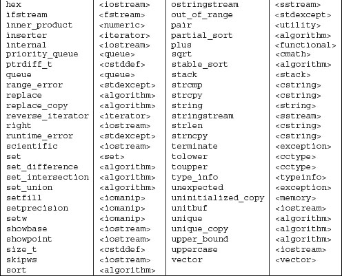
The second version applies the specified binary operations, using the first operation in place of addition and the second in place of multiplication. As an example, we might use inner_product to produce a list of parenthesized name–value pairs of elements, where the name is taken from the first input sequence and the corresponding value is in the second:
If the first sequence contains if, string, and sort, and the second contains keyword, library type, and algorithm, then the output would be
(if, keyword), (string, library type), (sort, algorithm)
partial_sum(beg, end, dest)
partial_sum(beg, end, dest, BinaryOp)
Writes a new sequence to dest in which the value of each new element represents the sum of all the previous elements up to and including its position within the input range. The first version uses the + operator for the element type; the second version applies the specified binary operation. The programmer must ensure that dest is at least as large as the input sequence. Returns the dest iterator incremented to refer just after the last element written.
Given the input sequence 0,1,1,2,3,5,8, the destination sequence will be 0,1,2,4,7,12,20. The fourth element, for example, is the partial sum of the three previous values (0,1,1) plus its own( 2), yielding a value of 4.
adjacent_difference(beg, end, dest)
adjacent_difference(beg, end, dest, BinaryOp)
Writes a new sequence to dest in which the value of each new element other than the first represents the difference of the current and previous element. The first version uses the element type’s - operation; the second version applies the specified binary operation. The programmer must ensure that dest is at least as large as the input sequence.
Given the sequence 0,1,1,2,3,5,8, the first element of the new sequence is a copy of the first element of the original sequence: 0. The second element is the difference between the first two elements: 1. The third element is the difference between the second and third element, which is 0, and so on. The new sequence is 0,1,0,1,1,2,3.
A.3 The IO Library Revisited
In Chapter 8 we introduced the basic architecture and most commonly used parts of the IO library. This Appendix completes our coverage of the IO library.
A.3.1 Format State
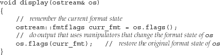
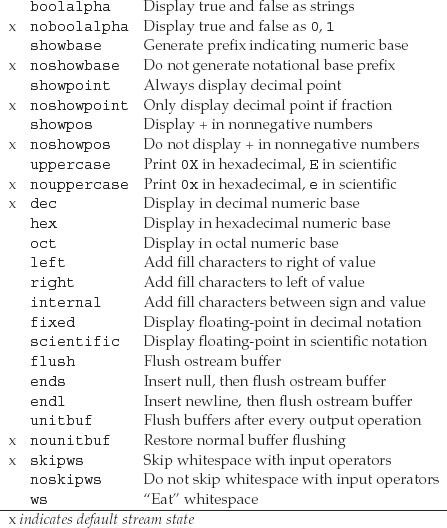
In addition to a condition state (Section 8.2, p. 287), each iostream object also maintains a format state that controls the details of how IO is formatted. The format state controls aspects of formatting such as the notational base for an integral value, the precision of a floating-point value, the width of an output element, and so on. The library also defines a set of manipulators (listed in Tables A.2 (p. 829) and A.3 (p. 833) for modifying the format state of an object. Simply speaking, a manipulator is a function or object that can be used as an operand to an input or output operator. A manipulator returns the stream object to which it is applied, so we can output multiple manipulators and data in a single statement.
When we read or write a manipulator, no data are read or written. Instead, an action is taken. Our programs have already used one manipulator, endl, which we “write” to an output stream as if it were a value. But endl isn’t a value; instead, it performs an operation: It writes a newline and flushes the buffer.
A.3.2 Many Manipulators Change the Format State
Many manipulators change the format state of the stream. They change the format of how floating-pointer numbers are printed or whether a bool is displayed as a numeric value or using the bool literals, true or false, and so forth.
Manipulators that change the format state of the stream usually leave the format state changed for all subsequent IO.
Most of the manipulators that change the format state provide set/unset pairs; one manipulator sets the format state to a new value and the other unsets it, restoring the normal default formatting.
The fact that a manipulator makes a persistent change to the format state can be useful when we have a set of IO operations that want to use the same formatting. Indeed, some programs take advantage of this aspect of manipulators to reset the behavior of one or more formatting rules for all its input or output. In such cases, the fact that a manipulator changes the stream is a desirable property.
However, many programs (and, more importantly, programmers) expect the state of the stream to match the normal library defaults. In these cases, leaving the state of the stream in a nonstandard state can lead to errors.

It is usually best to undo any state change made by a manipulator. Ordinarily, a stream should be in its ordinary, default state after every IO operation.
Using flags Operation to Restore the Format State
An even better approach to managing changes to format state uses the flags operations. The flags operations are similar to the rdstate and setstate operations that manage the condition state of the stream. In this case, the library defines a pair of flags functions:
• flags() with no arguments returns the stream’s current format state. The value returned is a library defined type named fmtflags.
• flags(arg) takes a fmtflags argument and sets the stream’s format as indicated by the argument.
We can use these functions to remember and restore the format state of either an input or output stream:
A.3.3 Controlling Output Formats
Many of the manipulators allow us to change the appearance of our output. There are two broad categories of output control: controlling the presentation of numeric values and controlling the amount and placement of padding.
Controlling the Format of Boolean Values
One example of a manipulator that changes the formatting state of its object is the boolalpha manipulator. By default, bool values print as 1 or 0. A true value is written as the integer 1 and a false value as 0. We can override this formatting by applying the boolalpha manipulator to the stream:
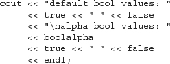
When executed, the program generates the following:
default bool values: 1 0
alpha bool values: true false
Once we “write” boolalpha on cout, we’ve changed how cout will print bool values from this point on. Subsequent operations that print bools will print them as either true or false.
To undo the format state change to cout, we must apply noboolalpha:
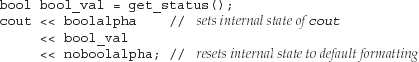
Now we change the formatting of bool values only to print of bool_val and immediately reset the stream back to its initial state.
Specifying the Base for Integral Values
By default, integral values are written and read in decimal notation. The programmer can change the notational base to octal or hexadecimal or back to decimal (the representation of floating-point values is unaffected) by using the manipulators hex, oct, and dec:

When compiled and executed, the program generates the following output:
default: ival = 15 jval = 1024
printed in octal: ival = 17 jval = 2000
printed in hexadecimal: ival = f jval = 400
printed in decimal: ival = 15 jval = 1024
Notice that like boolalpha, these manipulators change the format state. They affect the immediately following output, and all subsequent integral output, until the format is reset by invoking another manipulator.
Indicating Base on the Output
By default, when we print numbers, there is no visual cue as to what notational base was used. Is 20, for example, really 20, or an octal representation of 16? When printing numbers in decimal mode, the number is printed as we expect. If we need to print octal or hexadecimal values, it is likely that we should also use the showbase manipulator. The showbase manipulator causes the output stream to use the same conventions as used for specifying the base of an integral constant:
• A leading 0x indicates hexadecimal
• A leading 0 indicates octal
• The absence of either indicates decimal
Here is the program revised to use showbase:

The revised output makes it clear what the underlying value really is:
default: ival = 15 jval = 1024
printed in octal: ival = 017 jval = 02000
printed in hexadecimal: ival = 0xf jval = 0x400
printed in decimal: ival = 15 jval = 1024
The noshowbase manipulator resets cout so that it no longer displays the notational base of integral values.
By default, hexadecimal values are printed in lowercase with a lowercase x. We could display the X and the hex digits a—f as uppercase by applying the uppercase manipulator.
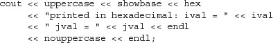
The preceding program generates the following output:
printed in hexadecimal: ival = 0XF jval = 0X400
To revert back to the lowercase x, we apply the nouppercase manipulator.
Controlling the Format of Floating-Point Values
There are three aspects of formatting floating-point values that we can control:
• Precision: how many digits are printed
• Notation: whether to print in decimal or scientific notation
• Handling of the decimal point for floating-point values that are whole numbers
By default, floating-point values are printed using six digits of precision. If the value has no fractional part, then the decimal point is omitted. Whether the number is printed using decimal or scientific notation depends on the value of the floating-point number being printed. The library chooses a format that enhances readability of the number. Very large and very small values are printed using scientific notation. Other values use fixed decimal.
Specifying How Much Precision to Print
By default, precision controls the total number of digits that are printed. When printed, floating-point values are rounded, not truncated, to the current precision. Thus, if the current precision is four, then 3.14159 becomes 3.142; if the precision is three, then it is printed as 3.14.
We can change the precision through a member function named precision or by using the setprecision manipulator. The precision member is overloaded (Section 7.8, p. 265): One version takes an int value and sets the precision to that new value. It returns the previous precision value. The other version takes no arguments and returns the current precision value. The setprecision manipulator takes an argument, which it uses to set the precision.
Table A.2. Manipulators Defined in iostream
The following program illustrates the different ways we can control the precision use when printing floating point values:
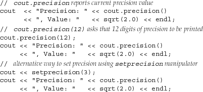
When compiled and executed, the program generates the following output:
Precision: 6, Value: 1.41421
Precision: 12, Value: 1.41421356237
Precision: 3, Value: 1.41
This program calls the library sqrt function, which is found in the cmath header. The sqrt function is overloaded and can be called on either a float, double, or long double argument. It returns the square root of its argument.

The setprecision manipulators and other manipulators that take arguments are defined in the iomanip header.
Controlling the Notation
By default, the notation used to print floating-point values depends on the size of the number: If the number is either very large or very small, it will be printed in scientific notation; otherwise, fixed decimal is used. The library chooses the notation that makes the number easiest to read.
When printing a floating-point number as a plain number (as opposed to printing money, or a percentage, where we want to control the appearance of the value), it is usually best to let the library choose the notation to use. The one time to force either scientific or fixed decimal is when printing a table in which the decimal points should line up.
If we want to force either scientific or fixed notation, we can do so by using the appropriate manipulator: The scientific manipulator changes the stream to use scientific notation. As with printing the x on hexadecimal integral values, we can also control the case of the e in scientific mode through the uppercase manipulator. The fixed manipulator changes the stream to use fixed decimal.
These manipulators change the default meaning of the precision for the stream. After executing either scientific or fixed, the precision value controls the number of digits after the decimal point. By default, precision specifies the total number of digits—both before and after the decimal point. Using fixed or scientific lets us print numbers lined up in columns. This strategy ensures that the decimal point is always in a fixed position relative to the fractional part being printed.
Reverting to Default Notation for Floating-Point Values
Unlike the other manipulators, there is no manipulator to return the stream to its default state in which it chooses a notation based on the value being printed. Instead, we must call the unsetf member to undo the change made by either scientific or fixed. To return the stream to default handling of float values we pass unsetf function a library-defined value named floatfield:
// reset to default handling for notation
cout.unsetf(ostream::floatfield);
Except for undoing their effect, using these manipulators is like using any other manipulator:
![]()
produces the following output:
1.41421
scientific: 1.414214e+00
fixed decimal: 1.414214
scientific: 1.414214E+00
fixed decimal: 1.414214
1.41421
Printing the Decimal Point
By default, when the fractional part of a floating-point value is 0, the decimal point is not displayed. The showpoint manipulator forces the decimal point to be printed:
![]()
The noshowpoint manipulator reinstates the default behavior. The next output expression will have the default behavior, which is to suppress the decimal point if the floating-point value has a 0 fractional part.
Padding the Output
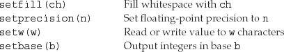
When printing data in columns, we often want fairly fine control over how the data are formatted. The library provides several manipulators to help us accomplish the control we might need:
• setw to specify the minimum space for the next numeric or string value.
• left to left-justify the output.
right to right-justfiy the output. Output is right-justified by default.
• internal controls placement of the sign on negative values. internal left-justifies the sign and right-justifies the value, padding any intervening space with blanks.
• setfill lets us specify an alternative character to use when padding the output. By default, the value is a space.
setw, like endl, does not change the internal state of the output stream. It determines the size of only the next output.
The following program illustrates these manipulators

When executed, this program generates
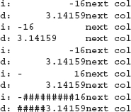
Table A.3. Manipulators Defined in iomanip
A.3.4 Controlling Input Formatting
By default, the input operators ignore whitespace (blank, tab, newline, formfeed, and carriage return). The following loop
![]()
given the input sequence
![]()
executes four times to read the characters a through d, skipping the intervening blanks, possible tabs, and newline characters. The output from this program is
abcd
The noskipws manipulator causes the input operator to read, rather than skip, whitespace. To return to the default behavior, we apply skipws manipulator:
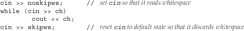
Given the same input as before, this loop makes seven iterations, reading white-space as well as the characters in the input. This loop generates
![]()
A.3.5 Unformatted Input/Output Operations
So far, our programs have used only formatted IO operations. The input and output operators (<< and >>) format the data they read or write according to the data type being handled. The input operators ignore whitespace; the output operators apply padding, precision, and so on.
The library also provides a rich set of low-level operations that support unformatted IO. These operations let us deal with a stream as a sequence of uninterpreted bytes rather than as a sequence of data types, such as char, int, string, and so on.
A.3.6 Single-Byte Operations
Several of the unformatted operations deal with a stream one byte at a time. They read rather than ignore whitespace. For example, we could use the unformatted IO operations get and put to read the characters one at a time:
![]()
This program preserves the whitespace in the input. Its output is identical to the input. Given the same input as read by the previous program that used noskipws, this program generates the same output:
![]()
Table A.4. Single-Byte Low-Level IO Operations
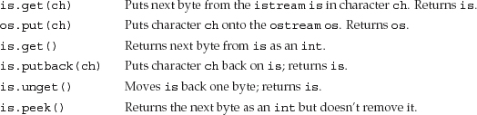
Putting Back onto an Input Stream
Sometimes we need to read a character in order to know that we aren’t ready for it yet. In such cases, we’d like to put the character back onto the stream. The library gives us three ways to do so, each of which has subtle differences from the others:
• peek returns a copy of the next character on the input stream but does not change the stream. The value returned by peek stays on the stream and will be the next one retrieved.
• unget backs up the input stream so that whatever value was last returned is still on the stream. We can call unget even if we do not know what value was last taken from the stream.
• putback is a more specialized version of unget: It returns the last value read from the stream but takes an argument that must be the same as the one that was last read. Few programs use putback because the simpler unget does the same job with fewer constraints.
In general, we are guaranteed to be able to put back at most one value before the next read. That is, we are not guaranteed to be able to call putback or unget successively without an intervening read operation.
int Return Values from Input Operations
The version of get that takes no argument and the peek function return a character from the input stream as an int. This fact can be surprising; it might seem more natural to have these functions return a char.
The reason that these functions return an int is to allow them to return an end-of-file marker. A given character set is allowed to use every value in the char range to represent an actual character. Thus, there is no extra value in that range to use to represent end-of-file.
Instead, these functions convert the character to unsigned char and then promote that value to int. As a result, even if the character set has characters that map to negative values, the int returned from these operations will be a positive value (Section 2.1.1, p. 36). By returning end-of-file as a negative value, the library guarantees that end-of-file will be distinct from any legitimate character value. Rather than requiring us to know the actual value returned, the iostream header defines a const named EOF that we can use to test if the value returned from get is end-of-file. It is essential that we use an int to hold the return from these functions:
This program operates identically to one on page 834, the only difference being the version of get that is used to read the input.
A.3.7 Multi-Byte Operations
Other unformatted IO operations deal with chunks of data at a time. These operations can be important if speed is an issue, but like other low-level operations they are error-prone. In particular, these operations require us to allocate and manage the character arrays (Section 4.3.1, p. 134) used to store and retrieve data.
The multi-byte operations are listed in Table A.5 (p. 837). It is worth noting that the get member is overloaded; there is a third version that reads a sequence of characters.
Caution: Low-Level Routines Are Error-Prone
In general, we advocate using the higher-level abstractions provided by the library. The IO operations that return int are a good example of why.
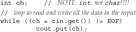
It is a common programming error to assign the return from get or one of the other int returning functions to a char rather than an int. Doing so is an error but an error the compiler will not detect. Instead, what happens depends on the machine and on the input data. For example, on a machine in which chars are implemented as unsigned chars, this loop will run forever:

The problem is that when get returns EOF, that value will be converted to an unsigned char value. That converted value is no longer equal to the integral value of EOF, and the loop will continue forever.
At least that error is likely to be caught in testing. On machines for which chars are implemented as signed chars, we can’t say with confidence what the behavior of the loop might be. What happens when an out-of-bounds value is assigned to a signed value is up to the compiler. On many machines, this loop will appear to work, unless a character in the input matches the EOF value. While such characters are unlikely in ordinary data, presumably low-level IO is necessary only when reading binary values that do not map directly to ordinary characters and numeric values. For example, on our machine, if the input contains a character whose value is ’377’ then the loop terminates prematurely. ’377’ is the value on our machine to which -1 converts when used as a signed char. If the input has this value, then it will be treated as the (premature) end-of-file indicator.
Such bugs do not happen when reading and writing typed values. If you can use the more type-safe, higher-level operations supported by the library, do so.
The get and getline functions take the same parameters, and their actions are similar but not identical. In each case, sink is a char array into which the data are placed. The functions read until one of the following conditions occurs:
• size - 1 characters are read
• End-of-file is encountered
• The delimiter character is encountered
Following any of these conditions, a null character is put in the next open position in the array. The difference between these functions is the treatment of the delimiter. get leaves the delimiter as the next character of the istream. getline reads and discards the delimiter. In either case, the delimiter is not stored in sink.
Table A.5. Multi-Byte Low-Level IO Operations

Determining How Many Characters Were Read
Several of the read operations read an unknown number of bytes from the input. We can call gcount to determine how many characters the last unformatted input operation read. It is esssential to call gcount before any intervening unformatted input operation. In particular, the single-character operations that put characters back on the stream are also unformatted input operations. If peek, unget, or putback are called before calling gcount, then the return value will be 0!
A.3.8 Random Access to a Stream
The various stream types generally support random access to the data in their associated stream. We can reposition the stream so that it skips around, reading first the last line, then the first, and so on. The library provides a pair of functions to seek to a given location and to tell the current location in the associated stream.
Random IO is an inherently system-dependent. To understand how to use these features, you must consult your system’s documentation.
Seek and Tell Functions
To support random access, the IO types maintain a marker that determines where the next read or write will happen. They also provide two functions: One repositions the marker by seeking to a given position; the second tells us the current position of the marker. The library actually defines two pairs of seek and tell functions, which are described in Table A.6. One pair is used by input streams, the other by output streams. The input and output versions are distinguished by a suffix that is either a g or a p. The g versions indicate that we are “getting” (reading) data, and the p functions indicate that we are “putting” (writing) data.
Table A.6. Seek and Tell Functions
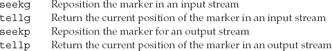
Logically enough, we can use only the g versions on an istream or its derived types ifstream, or istringstream, and we can use only the p versions on an ostream or its derived types ofstream, and ostringstream. An iostream, fstream, or stringstream can both read and write the associated stream; we can use either the g or p versions on objects of these types.
There Is Only One Marker
The fact that the library distinguishes between the “putting” and “getting” versions of the seek and tell functions can be misleading. Even though the library makes this distinction, it maintains only a single marker in the file—there is not a distinct read marker and write marker.
When we’re dealing with an input-only or output-only stream, the distinction isn’t even apparent. We can use only the g or only the p versions on such streams. If we attempt to call tellp on an ifstream, the compiler will complain. Similarly, it will not let us call seekg on an ostringstream.
When using the fstream and stringstream types that can both read and write, there is a single buffer that holds data to be read and written and a single marker denoting the current position in the buffer. The library maps both the g and p positions to this single marker.
Because there is only a single marker, we must do a seek to reposition the marker whenever we switch between reading and writing.
Plain iostreams Usually Do Not Allow Random Access
The seek and tell functions are defined for all the stream types. Whether they do anything useful depends on the kind of object to which the stream is bound. On most systems, the streams bound to cin, cout, cerr and clog do not support random access—after all, what would it mean to jump ten places back when writing directly to cout? We can call the seek and tell functions, but these functions will fail at run time, leaving the stream in an invalid state.
Because the istream and ostream types usually do not support random access, the remainder of this section should be considered as applicable to only the fstream and sstream types.
Repositioning the Marker
The seekg and seekp functions are used to change the read and write positions in a file or a string. After a call to seekg, the read position in the stream is changed; a call to seekp sets the position at which the next write will take place.
There are two versions of the seek functions: One moves to an “absolute” address within the file; the other moves to a byte offset from a given position:
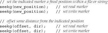
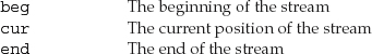
The first version sets the current position to a given location. The second takes an offset and an indicator of where to offset from. The possible values for the offset are listed in Table A.7.
Table A.7. Offset From Argument to seek
The argument and return types for these functions are machine-dependent types defined in both istream or ostream. The types, named pos_type and off_type, represent a file position and an offset from that position, respectively. A value of type off_type can be positive or negative; we can seek forward or backward in the file.
Accessing the Marker
The current position is returned by either tellg or tellp, depending on whether we’re looking for the read or write position. As before, the p indicates putting (writing) and the g indicates getting (reading). The tell functions are usually used to remember a location so that we can subsequently seek back to it:
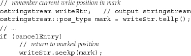
The tell functions return a value that indicates the position in the associated stream. As with the size_type of a string or vector, we do not know the actual type of the object returned from tellg or tellp. Instead, we use the pos_type member of the appropriate stream class.
A.3.9 Reading and Writing to the Same File
Let’s look at a programming example. Assume we are given a file to read. We are to write a new line at the end of the file that contains the relative position at which each line begins. For example, given the following file,
abcd
efg
hi
j
the program should produce the following modified file:
abcd
efg
hi
j
5 9 12 14
Note that our program need not write the offset for the first line—it always occurs at position 0. It should print the offset that corresponds to the end of the data portion of the file. That is, it should record the position after the end of the input so that we’ll know where the original data ends and where our output begins.
We can write this program by writing a loop that reads a line at a time:

This program opens the fstream using the in, out, and ate modes. The first two modes indicate that we intend to both read and write to the same file. By also opening it in ate mode, the file starts out positioned at the end. As usual, we check that the open succeeded, and exit if it did not.
Initial Setup
The core of our program will loop through the file a line at a time, recording the relative position of each line as it does so. Our loop should read the contents of the file up to but not including the line that we are adding to hold the line offsets. Because we will be writing to the file, we can’t just stop the loop when it encounters end-of-file. Instead, the loop should end when it reaches the point at which the original input ended. To do so, we must first remember the original end-of-file position.
We opened the file in ate mode, so it is already positioned at the end. We store the initial end position in end_mark. Of course, having remembered the end position, we must reposition the read marker at the beginning of the file before we attempt to read any data.
Main Processing Loop
Our while loop has a three-part condition.
We first check that the stream is valid. Assuming the first test on inOut succeeds, we then check whether we’ve exhausted our original input. We do this check by comparing the current read position returned from tellg with the position we remembered in end_mark. Finally, assuming that both tests succeeded, we call getline to read the next line of input. If getline succeeds, we perform the body of the loop.
The job that the while does is to increment the counter to determine the offset at which the next line starts and write that marker at the end of the file. Notice that the end of the file advances on each trip through the loop.
We start by remembering the current position in mark. We need to keep that value because we have to reposition the file in order to write the next relative offset. The seekp call does this repositioning, resetting the file pointer to the end of the file. We write the counter value and then restore the file position to the value we remembered in mark. The effect is that we return the marker to the same place it was after the last read. Having restored the marker, we’re ready to repeat the condition in the while.
Completing the File
Once we exit the loop, we have read each line and calculated all the starting offsets. All that remains is to print the offset of the last line. As with the other writes, we call seekp to position the file at the end and write the value of cnt. The only tricky part is remembering to clear the stream. We might exit the loop due to an end-of-file or other input error. If so, inOut would be in an error state, and both the seekp and the output expression would fail.