
Chapter 6
Transforming Pricing Management in a Chemical Supplier
Six Sigma is often assumed to be the prerogative of black belts, quality engineers, or continuous improvement professionals working in manufacturing environments where the culture and approach are amenable to the rigor and discipline of statistically based data analysis. This case study illustrates how Visual Six Sigma may be successfully applied in the world of sales and marketing, a world conventionally seen as being driven more by art and intuition than by data analysis and science. Specifically, we will see how Visual Six Sigma is used to drive a new way of conceptualizing and managing the pricing process of a multinational chemicals supplier.
Your employer, Polymat Ltd., is a manufacturer of polymeric materials that are sold into a range of commodity and specialty applications. Recently, Polymat has been facing growing competition from new manufacturing facilities, primarily in China and India. Market prices have declined steadily over a period of several years. Given your reputation as a skilled black belt, you are enlisted to help arrest the steady price decline.
You assemble a small team and construct what turns out to be a useful set of data. These data capture information from two sales campaigns that attempted to renegotiate prices so as to meet at least a 5 percent price increase. The campaigns cover two very different periods, one where Polymat's product was in undersupply and one where it was in oversupply. In addition to the actual percentage price increase that the sales representative was able to negotiate for each sale, the data set also includes ratings of the experience levels of the sales representative and buyer, as well as a classification of the value of each sale as seen from the buyer's point of view.
The two experience levels, together with the perceived value of the sale and a few other variables, constitute your Xs. Your Ys are percentage price increase and a nominal variable that reflects whether the target 5 percent increase was met. Failure to meet the 5 percent target defines a defect in the negotiating process.
Together with your team you explore these data, first assessing the capability of the pricing process and then uncovering relationships between the Xs and Ys. Given that one Y is continuous and the other is nominal, you use traditional modeling techniques as well as recursive partitioning to explore relationships with the Xs.
Guided by your data exploration, you identify several key areas for improvement: training of sales representatives, negotiating sales based on the knowledge of the product's value to the buyer, providing appropriate guidelines for sales managers, and accounting for the prevailing supply/demand balance when setting pricing targets. Addressing these areas leads to improvements in the pricing process, which your team continues to monitor over a period of time.
You and your team work through all of the steps of the Visual Six Sigma Data Analysis Process. Exhibit 6.1 lists the JMP platforms and options that you use in your analysis. The data sets are available at http://support.sas.com/visualsixsigma. This case study illustrates how Visual Six Sigma can lead to substantial improvements in sales and marketing.
Exhibit 6.1 Platforms and Options Illustrated in This Case Study
| Menus | Platforms and Options |
| Rows | Clear Row States |
| Color or Mark by Column | |
| Cols | Column Info |
| Column Properties | |
| Analyze | Distribution |
| Histogram | |
| Frequency Distribution | |
| Fit Y by X | |
| Contingency | |
| Oneway | |
| Means Diamonds | |
| Compare Means | |
| Fit Model | |
| Standard Least Squares | |
| Macros—Factorial to Degree | |
| Effect Summary | |
| Modeling | |
| Partition | |
| Decision Tree | |
| Quality and Process | Control Chart Builder |
| Diagram (Ishikawa C&E) | |
| Other | Local Data Filter |
SETTING THE SCENE
Polymat Ltd., headquartered in England, is a manufacturer of polymeric materials that are sold into a range of commodity and specialty applications. A leader in a steadily growing market, Polymat faces increased competition owing to large-scale competitive investments in new manufacturing facilities, primarily in China and India. As a consequence of the growing availability of product from these far eastern factories, market prices have shown a steady decline over a period of several years.
Bill Roberts is the recently appointed commercial director for Polymat. He has an excellent track record of business turnaround and has been appointed specifically to reverse Polymat's steady decline in profitability. During his first three months, Bill carries out a major review of each part of the Polymat business. He finds many things that concern him, but is particularly worried about the possibility of further price decline, because he knows that further significant cost cutting is not possible. In reviewing the situation with his colleagues, Bill realizes that despite several recent attempts to impose price increases, both margin and profitability have continued to be eroded.
Bill is aware that the market ultimately defines the price. However, having visited a number of customers, he has a hunch that his sales representatives are leaving money on the table in their price negotiations. Motivated by his recent attendance at an exciting conference on process management, Bill is determined to apply process thinking to this difficult challenge. He knows that new perspectives in sales and marketing are required to help Polymat halt or reverse the price decline. So he decides to go out and hire the best Six Sigma black belt he can find.
Being a highly experienced black belt trained in Visual Six Sigma, you are Bill's first choice and you quickly find yourself working for Polymat. Bill gives you very clear instructions: “Go out and fix my pricing process—it's broken!”
FRAMING THE PROBLEM: UNDERSTANDING THE CURRENT STATE PRICING PROCESS
You have a few key ideas in mind that help you focus your initial efforts. You realize that you need to form a team in order to have the relevant expertise available. You also need data in order to identify the root causes that will direct you to solutions. Your initial thinking is to design a data set using historical data.
In a previous project for another employer, you employed an approach based on a Product Categorization Matrix. This tool is based on the idea that the seller should view the product from the perspective of the buyer. You feel strongly that such a tool could put sales representatives in a stronger negotiating position for certain products. Consequently, you plan to integrate product categorization data into your team's investigation.
Defining the Process
Quickly, you pull together a small team consisting of two sales representatives, a sales clerk, and a Polymat financial analyst familiar with the IT system who knows how to access invoice and sales data. The team members agree that they should focus on improving the pricing management process—that is, the process that consists of setting price targets, negotiating prices with customers, and invoicing and tracking orders after a successful sale. To define the scope and focus of the initial work, the team starts by drawing a high-level map of this process (see Exhibit 6.2).

Exhibit 6.2 Process Map of Polymat's Price Management Process
When you review this scope with Bill, he confirms that this is the right place to start. His management team is already undertaking a strategic review of the market planning process and is looking to simplify Polymat's product range. Bill makes it clear that he expects you to help drive improvement in the operational implementation of the stipulated market plans and pricing strategies. This is where he believes a Six Sigma approach will be most beneficial.
Based on discussions with Bill and other members of the management team, you also realize that recent attempts to renegotiate prices with customers have by and large been unsuccessful. Working with the financial analyst on your team, you uncover data connected to four separate attempts to increase prices over the last two years. Each of these was directed at achieving a 5 percent price increase across Polymath's customer base. None of the four attempts were successful in meeting this target.
Constructing an Analysis Data Set
In thinking about your analysis data set, you decide that your primary Y will be a measure of the price increase. For each sale, you define this as the difference between the price charged for the product after the negotiated increase and the price that would have been charged before the increase, divided by the price before the increase. This measure eliminates any currency exchange rate fluctuations that might otherwise complicate the analysis.
You also realize that prevailing market conditions have a pronounced effect on price. The market for Polymat products is highly volatile and can change from demand exceeding supply (a shortage) to supply exceeding demand (an oversupply) in just six to twelve months, depending on a number of factors:
- Cyclical characteristics of end user markets (e.g., packaging, electronics)
- Fluctuating oil prices (a key raw material)
- New polymer supply factories coming online (mainly in China and the Far East)
Based simply on market forces, you expect that when demand exceeds supply, a higher price should be viable (and vice versa). However, you need to verify that this expectation is supported by the data. So, to better understand the situation, you decide to baseline the capability of the current pricing management process using a detailed assessment of two of the recent attempts to impose a unilateral price increase.
After intensive planning and some brainstorming with the team to identify useful data for this investigation, it becomes clear that information on the experience of the sales representative and on the sophistication of the buyer involved in each sale will be vital. With this in mind, you realize that it does not make sense simply to use a large set of unstructured and possibly uninformative sales data. Instead, you decide to retroactively design and assemble a data set for your baseline assessment. This will both ensure that you have data on the relevant background variables and minimize the time you spend researching and constructing the values of related variables.
You construct the data set for the baseline assessment as follows:
- Products. Working with a member of the Polymat marketing department, you select 20 products as the basis for the study. These products represent a range of both commodity and specialty product types as defined in the Polymat marketing plan. The products are sold in volume and have a respectable (>30 percent) combined market share.
- Customers. Polymat is the market leader in four territories: the United Kingdom, France, Germany, and Italy. You want to ensure that the study includes a range of customers from each of these territories. To that end, for each of the 20 products, 3 customers representing a range of different sizes are chosen from each of the 4 regions. Here, customer size is defined as the annual volume in sales made by Polymat to that customer. A total of 240 customers are represented: three customers for each of 20 products for each of four regions.
- Supply/Demand Balance. To include the effect of market conditions in the analysis, you identify two price increase campaigns that were run under different conditions. In the first case, the market was tight; that is, demand was close to exceeding supply, and there was a relative shortage of polymer product. In the second case, 12 months later, the market had shifted to a point where, owing to new factories coming online, there was oversupply.
Based on this retroactive design, you construct a data table whose rows are defined by all possible combinations of the 20 products, the 12 customers (three in each of the four regions), and the two supply/demand balance periods. This leads to 20 × 12 × 2 = 480 records. For each of the combinations of product, customer, and supply/demand balance period, you obtain the following information for a sale:
- Sales Representative Experience. You believe that the experience of the sales representative is a factor of interest, because at Polymat there is no fixed price for each product. Sales representatives have the responsibility of negotiating the best price based on general guidelines and pricing targets set by their sales manager. Consequently, the price that a customer pays for a product depends on the outcome of the negotiation with the buyer. The sales manager helps you to classify the sales representatives into three categories of experience: high, medium, and low. The classification is based on each representative's number of years of general sales experience and his or her industry-specific knowledge. For example, a sales representative designated with high experience has more than ten years of sales experience and in excess of five years selling at Polymat or a similar business.
- Buyer Sophistication. Because negotiation is a two-way undertaking, you want to explore the relationship between the experience of the sales representative and the experience of the buyer. You expect that price negotiations will differ based on whether an inexperienced sales representative is selling to an experienced and skilled buyer, or vice versa. You sit down with the sales manager to categorize the buyer sophistication for each customer that bought one of the 20 products under consideration. High buyer sophistication is allocated to customers whose buyers are highly professional and highly trained, whereas low buyer sophistication is assigned to customers whose buyers are less highly trained or skilled.
- Product Category. This is a categorization of a product and customer into one of four classes, based on how the buying organization views and uses the product. The Product Categorization Matrix section that follows describes this categorization and your use of it.
- Annual Volume Purchased. This is the total amount spent by each customer for this product over the year in which the supply/demand balance period falls.
- % Price Increase (Y). This is computed by taking the difference between the price charged for the product after the negotiated increase and the price that would have been charged before the increase, and dividing this difference by the price before the increase.
Product Categorization Matrix
You are concerned about the simple specialty–commodity split that marketing uses to describe Polymat's products. Luckily, in a previous role, you were responsible for a project in which purchasing operations were redesigned. As part of that project, you developed a simple tool to encourage buyers to think differently about what they did, where they spent their time, and where they should focus to reduce the costs of the products they bought.
You decide to turn this thinking on its head and apply the same idea to Polymat's pricing process. “After all,” you reflect, “if you are selling a product and want to get the best price, it's certainly a good idea to think of the product and its value in the same way that a customer would.”
You pull the team members together over lunch for a discussion of your proposed approach. You explain that the Product Categorization Matrix will help everyone to see the product from the buyer's viewpoint, and so should be more informative than the specialty–commodity split that just sees things from the seller's point of view. You go on to say that each sale (of a product to a customer) can be placed into a two-by-two grid based on the requirements of the buying organization (Exhibit 6.3).

Exhibit 6.3 The Product Categorization Matrix
The vertical axis, Alternative Sources of Product, represents the buyer's supply vulnerability relative to the product in question. The axis is scaled from Few to Many, referring to the number of potential suppliers. It represents the buyer's risk, posing the question, “What happens if the current seller cannot provide the product?” For example, if the buyer cannot obtain an equivalent product elsewhere, or if the product is specific to the buyer's process, then that sale's value on Alternative Sources of Product is Few.
The horizontal axis, Product Volume Purchased, represents the product's relative cost to the buyer. This axis is scaled from Low to High. If a product represents a high proportion of the buyer's spend, the Product Volume Purchased rating of the sale is High.
The four quadrants of the matrix are:
- Strategic Security. This quadrant contains products for which the buyer has few alternatives. These products may be unique or specific to the customer's process but represent a low proportion of the buyer's spending. These products should be able to command a high price and the buyer should be relatively insensitive to price increases. The key task of the buyer is to ensure the security of his business by guaranteeing a supply of these strategic products almost at any cost.
- Strategic Critical. This quadrant contains products for which the buyer's spending is very high. Small changes in price will have a high impact on the buyer's overall spending. Therefore, the buyer will typically be more sensitive to price. The critical task of the buyer is to purchase these strategic products at minimal cost.
- Tactical Profit. For products in this quadrant, the buyer has several options, as there are competitive products with similar characteristics available from alternative vendors. The product in this category represents a high proportion of the buyer's spending, so the buyer will make tactical purchasing decisions based on maximizing his profit. In marketing terms, products in this category are typical commodity products. There is little differentiation and high price sensitivity—hence, it will be very difficult to increase the price for these products. Any attempt to do so will encourage the buyer to purchase from a competitor and the business will be lost.
- Non Critical. Products in this quadrant are commodity products that represent small-volume purchases for the buyer. There are many equivalent products available, and the products represent a small overall cost. Decisions regarding the purchase of these products will be based on criteria other than price, such as ease of doing business, lead time, and similar factors.
The buyer will typically expend effort in two areas of the matrix: the Strategic Security products and the Strategic Critical products. The buyer will be sensitive to price in two areas: Strategic Critical and Tactical Profit. The buyer's ultimate strategy is to move all of his products to the Tactical Profit quadrant, where he can play one supplier against another, or at least to make his suppliers believe that their products are in this quadrant!
As you emphasize, this product categorization is based on the use of the product. A particular product may be Strategic Security for customer A because alternative products do not give the same consistency of performance in customer A's manufacturing process, whereas for customer B, that same product may be Non Critical, being one of several alternatives that can deliver the consistency that customer B requires.
As the team quickly realizes, this approach to thinking about price sensitivity is situational—it is quite different from simply setting a list price for each product—and will give Polymat's sales representatives greater insight into the price increase a specific transaction may bear. With the team's support, you hold a series of meetings with the appropriate sales and marketing personnel to apply their account knowledge in categorizing the transactions included in the baseline data set. When this work is completed, you are happy to see that all four types of sale are broadly represented in the baseline data.
COLLECTING BASELINE DATA
Now you and your team embark on the process of obtaining the historical data and verifying its integrity. Once this is done, you will compute some baseline measures.
Obtaining the Data
From the two periods during which 5 percent price increases were targeted, you have identified 20 products and, for each product, 12 customers representing various sizes and regional locations (three customers per region). Each of these product and customer combinations had sales in each of two periods: oversupply and shortage. This results in 480 different product-by-customer-by-period combinations.
The invoice figures for these sales are directly downloaded from Polymat's data warehouse into a standard database. After entering the Product Categorization Matrix categories determined earlier, along with the sales representative experience and buyer sophistication rankings, you load the data from the two pricing intervention periods into JMP for further investigation. The raw data are given in the first ten columns in the 480-row data table BaselinePricing.jmp (Exhibit 6.4).

Exhibit 6.4 Partial View of Baseline Pricing Data Table
You have heard some members of the management team refer to a failure to achieve a 5 percent increase as a pricing defect. This makes sense to you, so you add an 11th column to the data table that indicates whether the given sale has this defect. For your current purposes, you will consider any sale that exhibits a pricing defect to be defective.
You call your new column Defective, and you define it using a formula. Once you have defined the column using JMP's Formula Editor, a plus sign (+) appears next to the column name in the Columns panel to the left of the data grid. Clicking on the plus sign shows you the formula. You foresee using this column as an easy categorization of whether the price obtained for the given sale met the mandated increase.
The columns in the data table are described in Exhibit 6.5. Note that only the last two variables are Ys. The rest are Xs that you believe may be useful in your understanding of the resulting price increases. You assign appropriate data modeling types to your variables: Most are nominal, but Sales Rep Experience and Buyer Sophistication are ordinal while Annual Volume Purchased and % Price Increase are continuous.
Exhibit 6.5 Description of Columns in the Baseline Pricing.jmp Data Table
| Column | Description |
Product Code |
Product identifier |
Region |
Region of facility making the purchase |
Customer ID |
Customer identifier |
Supply Demand Balance |
Prevailing market conditions when a price increase was made (Shortage or Oversupply) |
Sales Rep |
Name of sales representative |
Sales Rep Experience |
Sales representative's experience level |
Buyer Sophistication |
Customer's level of buying sophistication |
Product Category |
Category of product when sold to a particular customer |
Annual Volume Purchased |
Total amount spent by the customer for this product over the year in which the supply/demand balance period falls |
% Price Increase |
Percentage price increase defined as 100 x (Price After – Price Before)/Price Before, where Price After = invoiced price after the price increase was implemented, and Price Before = invoiced price before the price increase was implemented |
Defective |
Categorization as defective when the % Price Increase is <= 5% and not defective otherwise |
Verification of Data Integrity
You begin your analysis with a quick check to make sure that the data you have imported into JMP are what you expect. You also want to check that the incidence of the categories in your nominal variables is large enough to allow useful analysis. For example, if only 2 percent of records were not defective, then the data would be of questionable value in helping to determine which Xs affect the response Defective. There would simply not be sufficiently many records with a nondefective outcome.
To take a quick look at your data, you use the Distribution platform to analyze all of your columns.
From the first four reports, you verify that your 20 product codes, 4 regions, 240 customers, and 2 periods of supply/demand balance are represented in equal proportions. You look at the remaining reports to learn that:
Sales Rep: A reasonable number of sales representatives are represented.Sales Rep Experience: The experience levels of these sales representatives span the three categories, with reasonable representation in each.Buyer Sophistication: Buyers of various sophistication levels are represented in almost equal proportions.Product Category: Each of the four product categories is well-represented, with the smallest having a 17.5 percent representation.Annual Volume Purchased: The distribution of volume purchased for these products is consistent with what you expected.% Price Increase: This shows a slightly right-skewed distribution, which is to be expected, with a mean of 3.7 percent—you will analyze this Y further once you finish verifying the data.Defective: This shows that about 72 percent of all records are defective (according to the 5 percent cutoff) and that 28 percent are not. This representation in the two groupings is adequate to allow further analysis.
Just in passing, you notice that JMP does something very nice in ordering the categories for nominal variables. The default is for JMP to list these in alphabetical order in plots; for example, the Sales Rep names are listed in reverse alphabetical order in the plot and in direct order in the frequency table in Exhibit 6.6. But JMP uses some intelligence in ordering the categories of Sales Rep Experience and Buyer Sophistication. Both have Low, Medium, and High categories, which JMP places in their context-based, rather than alphabetical order.
You conclude from this analysis that your data are consistent with your intended design and that the distributions of the nondesigned variables make sense and provide reasonable representation of the categories of interest. Now you initiate your baseline analysis.
Baseline Analysis
The purpose of your baseline analysis is to understand the capability of the current pricing management process under the two different market conditions of Oversupply and Shortage. You have already seen that the overall defect rate is about 0.72. An easy way to break this down by the two Supply Demand Balance conditions is to construct a mosaic plot and contingency table (Exhibit 6.7).

Exhibit 6.7 Contingency Report for Defective
You see immediately that the percentage of defective sales is much larger in periods of Oversupply than in periods of Shortage, as represented by the areas in the Mosaic Plot (these appear blue on a computer screen). Click in the report and then place your cursor over each rectangular area in the mosaic plot to see the percentage (called Frequency) of sales represented by the rectangle.
The Contingency Table below the plot gives the Count of records in each of the classifications as well as the Row %. You see that in periods of Oversupply, about 86 percent (specifically, 85.83 percent) of the sales in your data table are defective, while in periods of Shortage, about 58 percent (specifically, 57.92 percent) are defective.
This finding makes sense. However, if you relate what you see to the expectation of Polymat's leadership team, you start to understand some of Bill Roberts's frustrations. Even in times of Shortage, when the account managers are in a strong negotiating position, Polymat suffers a high pricing defect rate—an estimated 58 percent of the sales negotiations are defective.
Recreate the Distribution report for % Price Increase by running the script Distributions. Select the option Display Options > Horizontal Layout from the red triangle menu next to % Price Increase to obtain the layout shown in Exhibit 6.8. The Summary Statistics report shows a mean overall increase of 3.7 percent. The Quantiles report indicates that the price increases vary quite a bit, from 0 percent to about 9.3 percent.

Exhibit 6.8 Distribution Report for % Price Increase
But what about the breakdown by Supply Demand Balance? Again, you want to see the relationship between a Y, % Price Increase, and an X, Supply Demand Balance (Exhibit 6.9).

Exhibit 6.9 Oneway Report for % Price Increase by Supply Demand Balance
The plot shows that % Price Increase is higher in periods of Shortage than in periods of Oversupply. This is not unexpected. The range of % Price Increase is fairly large in both periods. The Means and Standard Deviations report shows that, in periods of Oversupply, the mean % Price Increase is about 2.7 percent while in periods of Shortage it is 4.7 percent. Both means are below the desired 5 percent increase, with a much lower mean during periods of Oversupply.
Yet this is an exciting initial finding. There is a high potential for improvement if the business can increase prices when market conditions are advantageous. You immediately use your baseline analysis to entice Polymat's senior staff to increase their commitment to the project. Recognizing the power of appropriate language to change behavior, you also start to reinforce the concept of a pricing defect within the leadership team. You are pleasantly surprised by how quickly Bill starts to use this language to drive a new way of thinking.
UNCOVERING RELATIONSHIPS
You are anxious to embark on the task of identifying Hot Xs. But first, you take a little time to think through how you will structure the analysis of your data. You think back to the Visual Six Sigma Data Analysis Process (Exhibit 3.29) and observe that you are now at the Uncover Relationships step, which, if necessary, is followed by the Model Relationships step. Referring to the Visual Six Sigma Roadmap (Exhibit 3.30), you decide to do the following:
- Use the
Distributionplatform and dynamic visualization to better understand potential relationships among the variables. - Plot the variables two at a time to determine if any of the Xs might have an effect on the Ys.
- Use multivariate visualization techniques to explore higher-dimensional relationships among the variables.
If you find evidence of relationships using these exploratory techniques, and if you can corroborate this evidence with contextual knowledge, you could stop your analysis here. You would then proceed directly to proposing and verifying improvement actions as part of the Revise Knowledge step. However, since your data set is not very large, you decide that before moving to Revise Knowledge you will follow up with the Model Relationships step to try to confirm the hypotheses that you obtain from data exploration.
Dynamic Visualization of Variables Using Distribution
To explore which Xs might be influencing the Ys, you rerun your Distributions script. Now you use dynamic linking in the Distribution platform to identify the Xs that might influence the success or the lack of success of the two historical price increases under investigation.
In the Distribution plot for Defective, click in the No bar. (See Exhibit 6.10.) This has the effect of selecting all those rows in the data table where Defective has the value No. In turn, this highlights the areas that represent these points in all of the other Distribution plots. Note that the graph for Customer ID is only partially shown in Exhibit 6.10, as it involves 240 bars.

Exhibit 6.10 Highlighted Portions of Distributions Linked to Defective = No
As you toggle between the Yes and No bars for Defective you see that Supply Demand Balance, Buyer Sophistication, and Product Category have different distributions based on whether Defective is Yes or No. It also appears that Defective may be related to Product Code and Customer ID. This raises the question of how, in terms of root causes, these last two variables might affect pricing defects. You believe that the causal link relates to how the customer views the product. The root cause may be related to the Product Category as assigned using the Product Categorization Matrix.
By interacting with the Defective bar chart in this way, you also learn that price increase has little or no association with:
Region. Whether a price increase is defective does not appear to depend on region.Sales Rep. There is some variation in how sales representatives perform, but there is no indication that some are strikingly better than others at achieving the target price increases.Sales Rep Experience. Interestingly, the highly experienced account managers appear to be no more effective in increasing the price than those who are less experienced. (This is much to everyone's surprise.)Annual Volume Purchased. Sales representatives appear to be no better at raising prices with small customers than with large customers.
You also want to see the impact of Product Category on pricing defects. In the Product Category plot, you want to highlight both the Strategic Security and Strategic Critical bars. To do this, first click in the Strategic Security bar. Then hold the Control key while you click in the Strategic Critical bar. The impact on Defective is shown in Exhibit 6.11.

Exhibit 6.11 Impact of Strategic Product Categories on Defective
Note that almost all of the sales that met the price increase target, namely, where Defective has the value No, come from these two categories. Alternatively, clicking on the No bar in the Defective graph shows that almost all of these sales are either Strategic Security or Strategic Critical. This supports your belief that Product Category captures the effect of Product Code and Customer ID.
However, the most interesting X appears to be Buyer Sophistication. Select High values of Buyer Sophistication by clicking on the appropriate Distribution plot bar. After examining the other plots, click on the Medium and Low values. With highly sophisticated buyers, the proportion of pricing defects is much higher than for buyers who have Medium or Low sophistication. You conclude that these buyers use highly effective price negotiations to keep prices low (Exhibit 6.12).

Exhibit 6.12 Impact of High Buyer Sophistication on Defective
To date, your exploratory analysis leaves you suspecting that the main Xs of interest are Supply Demand Balance, Buyer Sophistication, and Product Category. Although you have simply run Distribution analyses for your variables, you have used dynamic linking to study your variables two at a time by viewing the highlighted or conditional distributions. In the next section, you use Fit Y by X to continue viewing your data two variables at a time.
Dynamic Visualization of Variables Two at a Time
You have already used the Fit Y by X platform, found under Analyze, in your baseline analysis. As you know, Fit Y by X provides reports that help identify relationships between pairs of variables. You want to get a better look at how Supply Demand Balance, Buyer Sophistication, and Product Category are related to Defective.
In the report window the contingency tables that are shown by default include Total % and Col %. But you are only interested in Count and Row %. You would like to remove Total % and Col % from all three analyses. You also would prefer not to have to go through the keystrokes to do this individually for all three reports.
In most report windows, JMP allows you to run through the keystrokes once and have the commands broadcast to all similar reports. Simply hold the Control key while selecting the desired menu options. This applies your selections to all other similar objects in the report.
The plots and contingency tables show:
Supply Demand Balance. Not surprisingly, there are fewer defective sales in periods of Shortage than in periods of Oversupply: 58 percent versus 86 percent, respectively. (Note that this is the same plot as in Exhibit 6.7.)Buyer Sophistication. There are more defective sales when dealing with highly sophisticated buyers (90 percent) than when dealing with buyers of medium or low sophistication (about 61 percent for each group). In fact, there appears to be little difference between low- and medium-sophistication buyers relative to defective sales, although other variables might differentiate these categories.Product Category. This has a striking impact on defective sales. The defective rates for Strategic Critical and Strategic Security are 56 percent and 47 percent, respectively, compared to Non Critical and Tactical Profit, with defective rates of 92 percent and 94 percent, respectively.
This analysis is conducted with the nominal response, Defective. You realize that the variable Defective is simply a coarsened version of the continuous variable % Price Increase. Will these results carry through for the continuous response, % Price Increase?
Exhibit 6.14 shows you the distributions across the levels of each variable. You see what appear to be differences across the levels of each X.

Exhibit 6.14 Three Oneway Reports for % Price Increase
But you would also like a statistical guide to determine which levels differ. You know that the Compare Means option, obtained from the red triangle menu, constructs Comparison Circles. These provide a visual representation of a statistical test for significant differences among the levels of the Xs.
When you choose Compare Means you will notice four options. The two most often used are Each Pair, Student's t and All Pairs, Tukey HSD. The difference between these two procedures is that the Each Pair option controls the risk of incorrectly concluding that two specific groups differ, whereas the All Pairs option controls this risk for all possible comparisons of two groups. The default level for both risks is 5 percent. The All Pairs, Tukey HSD option is the more conservative, and for this reason, you choose to use this option. (It generally makes sense to use the All Pairs, Tukey HSD option unless you have good reason not to.)
The resulting report, except for the coloring of the comparison circles, is shown in Exhibit 6.15. The report shows plots with means diamonds overlaid on the jittered points. The central horizontal line in each of these diamonds is plotted at the level of the sample mean for % Price Increase for that category. The top and bottom of each diamond defines a 95 percent confidence interval for the true category mean. Looking at these, you realize that there are probably a number of statistically significant differences. For each variable, a table of means and standard deviations for each grouping is given below the plot.

Exhibit 6.15 Reports Showing Means Diamonds and Comparison Circles
The plot in Exhibit 6.15 shows an area to the right of the points containing comparison circles. These circles are a graphical way to test for differences in the means of the levels of each predictor.
For example, take Product Category, which has four levels. There is one circle corresponding to each level. The top two circles in the plot for Product Category in Exhibit 6.15 correspond to the levels Strategic Security and Strategic Critical.
Click on the smaller of the two top circles. The Strategic Security label on the horizontal axis changes to red (given the default JMP settings) and is given in boldface type. Meanwhile, the circle for Strategic Critical changes to red but is not bolded. (See Exhibit 6.15.)

Exhibit 6.16 Initial Partition Report with Split Probabilities and Counts
Since both circles are red, this means that the mean % Price Increase does not differ significantly for these two levels. However, the circles for Non Critical and Tactical Profit are gray. This means that the mean % Price Increase for each of these two categories differs significantly from the mean % Price Increase for Strategic Security, the bolded category.
Now click on the larger of the two top circles. This selects the Strategic Critical circle and its label appears in boldface text, while the label for Strategic Security is not bolded. This again indicates that these two groups do not differ statistically. The other two labels, Non Critical and Tactical Profit, are in non-boldface, italicized text, indicating that these two do differ statistically from Strategic Critical.
For Supply Demand Balance, Oversupply is selected in Exhibit 6.15. The two circles corresponding to Oversupply and Undersupply do not overlap. This indicates that the two groups differ statistically in their effect on % Price Increase.
For Buyer Sophistication, High-sophistication buyers are selected in Exhibit 6.15. High-sophistication buyers differ statistically in their effect on % Price Increase from Medium- and Low-sophistication buyers. By clicking on the circle for Medium-sophistication buyers, you see that the Medium- and Low-sophistication groups do not differ statistically.
Continuing your analysis, you click on circles corresponding to other levels of variables in Exhibit 6.15 one by one to see which differ relative to % Price Increase. Recalling that two categories differ with statistical significance only if, when you click on one of the circles, the other changes to gray, you conclude that:
- The mean
% Price Increasediffers significantly based on theSupply Demand Balance, with higher increases in periods of Shortage. - The mean
% Price Increasefor HighBuyer Sophisticationis significantly lower than for Medium- or Low-sophistication levels, whereas these last two do not differ significantly. - The mean
% Price Increasefor the Strategic Critical and Strategic SecurityProduct Categorylevels are significantly higher than for the Non Critical and Tactical Profit levels, although the means for Strategic Critical and Strategic Security do not differ significantly. - The mean
% Price Increasefor the Non Critical products is significantly higher than for the Tactical Profit products.
The Means Comparisons reports, whose disclosure icons are closed in Exhibit 6.15, are analytic reports containing the results that give rise to the comparison circles. For exploratory purposes, it suffices to examine the comparison circles.
You realize that you have identified which X category levels differ with statistical significance. Practical importance is quite another matter. In the report (Exhibit 6.15), you study the actual means and their confidence intervals. For example, relative to Buyer Sophistication, you note that High-sophistication buyers had mean % Price Increase values of about 2.7 percent, with a confidence interval for the true mean ranging from about 2.4 to 2.9 percent (Lower 95% and Upper 95% refer to the confidence interval limits). For less sophisticated buyers, these increases are much higher—about 4.3 percent for Medium- and 4.4 percent for Low-sophistication levels. In a similar fashion, you study the means and confidence intervals for the other Xs.
This exploratory Fit Y by X analysis provides you with evidence that there are differences in % Price Increase based on a number of levels of these three Xs. Given this evidence, you are comfortable thinking of Supply Demand Balance, Buyer Sophistication, and Product Category as Hot Xs for the continuous Y, % Price Increase. Of course, you need to verify that these are indeed Hot Xs. You realize that there may well be interactions among the potential Xs and that these will not be evident without a multivariate analysis. To that end, you now proceed to explore multivariate relationships among these variables.
Dynamic Visualization of Several Variables at a Time
The Initial Partition Report
Your Fit Y by X analysis looks at one X at a time in relation to the Ys. This means that your conclusions to date may overlook joint relationships among the Xs and a Y. You have a nominal Y, Defective, and a continuous Y, % Price Increase. You could explore Defective using logistic regression or a partition analysis. But because of its ease of interpretation and the fact that you have several nominal Xs, some of which have many levels, you decide to use the Partition platform.
Your use of Partition will be for exploration rather than modeling. There will be no statistical hypothesis tests, so validation of any conclusions you reach will need to rely on contextual knowledge of the process and on data that you collect in the future. (Note that later on, to study % Price Increase, you will use a multiple linear regression model, using Fit Model. This will provide some confirmatory analysis from modeling, and also reveals a new insight.)
Changing Colors
“But wait a minute,” you think. “This coloring sends the wrong message: Points corresponding to nondefective sales are colored red (a color associated with danger), while the points corresponding to defective sales are colored blue.” You decide it would be better, especially for the purpose of presenting your results, if the points corresponding to nondefective sales were always colored green and those corresponding to defective sales were always colored red.
To make this happen, you define a Column Property, namely a property associated with a column or variable. The property you will define is called a Value Colors column property.
In the data table, the rows have the red or green row state indicators to the left of the row numbers. Also, the cells in the column Defective are colored red and green. The plot in the partition report shows the new colors.
Splitting
Now you are ready to start splitting your data into groups or nodes that differentiate between defective and nondefective sales. At each split step, the partition algorithm finds the variable that best explains the difference between the two levels of Defective. The two groupings of values that best explain this difference are added as nodes to the diagram, so that repeated splits of the data produce a tree-like structure.
You realize that you can split as many times as you like, with the only built-in constraint being the minimum size split. This is the size of the smallest split grouping that is allowed. To see where this is set by default, click on the red triangle at the top of the report and select Minimum Size Split. The dialog window that appears indicates that the minimum size is set at five.
With 480 records, you think this might be small. It could allow for overfitting the data, namely, modeling noise rather than structure. After some thought, you decide to specify a minimum size of 25 for your splits. This should help ensure that your analysis reveals true structure, rather than just the vagaries of this specific data set. So you enter 25 as the Minimum Size Split in the dialog window and click OK.
Note that you could also use a Validation Portion, which is an option on the launch window, to avoid overfitting. This would be the better approach if you were interested in a predictive model. However, in this case study, you are interested in data exploration, so controlling splitting with a minimum size split is a reasonable approach.
Now you are ready to begin splitting. Click once on the Split button to obtain the report in Exhibit 6.18. The first split is on the variable Customer ID. You see that for a large group of customers all sales are defective, while for the other group of customers only about 33 percent of sales are defective.

Exhibit 6.18 Partition with One Split on Customer ID
However, the variable Customer ID, in its current state, is not useful for understanding the root causes of defective sales. Perhaps if you had combined customer IDs into broad categories, the binned version of Customer ID might be useful. For this reason, you regret having included Customer ID as a predictor. But, you do not need to start your analysis over. Instead, click on the top red triangle and select Lock Columns. The tooltip for the option points out that this will allow you to lock the Customer ID column out of your analysis.
Selecting Lock Columns inserts a list of the Xs to the right of the plot at the top of the report. In this list, check Customer ID. Then click the Prune button to remove the split on Customer ID from the report (Exhibit 6.19).

Exhibit 6.19 Locking Out Customer ID
Now you are ready to split once more. Clicking Split once provides a split on Product Category (Exhibit 6.20). You see that the two categories Tactical Profit and Non Critical result in a 93 percent defective rate (the node on the left). The Strategic Critical and Strategic Security categories have a 50 percent defective rate (the node on the right). These proportions are reflected in the plot above the tree. You hope that further splits will help explain more of the variation currently left unexplained, especially within the node on the right.

Exhibit 6.20 Partition with First Split on Product Category
A second split brings Buyer Sophistication into play (Exhibit 6.21). For the Strategic Critical and Strategic Security product categories, High-sophistication buyers are associated with an 82 percent rate of defective sales, while Medium- and Low-sophistication buyers are associated with a 30 percent rate. This is fantastic information, reinforcing the notion that for high-profile product categories, Polymat's sales representatives need to be better equipped to deal with highly sophisticated buyers.

Exhibit 6.21 Partition with Two Splits
At this point, you decide to split until the stopping rule, a minimum node size of 25, ends the splitting process. Repeatedly click on Split as you monitor the Number of Splits in the information panel to the right of the Split and Prune buttons. As a result of the specified minimum size split, splitting stops after nine splits.
The tree is now so big that it no longer fits on your screen. You have to navigate to various parts of it to see what is going on.
Click the top red triangle menu and select Small Tree View. A small tree (Exhibit 6.22) appears to the right of the plot and Lock Columns list. This small tree allows you to see the columns where splits have occurred, but it does not give the node detail. However, with the exception of Region (bottom, middle), the splits are on the three variables that you have been thinking of as your Hot Xs.
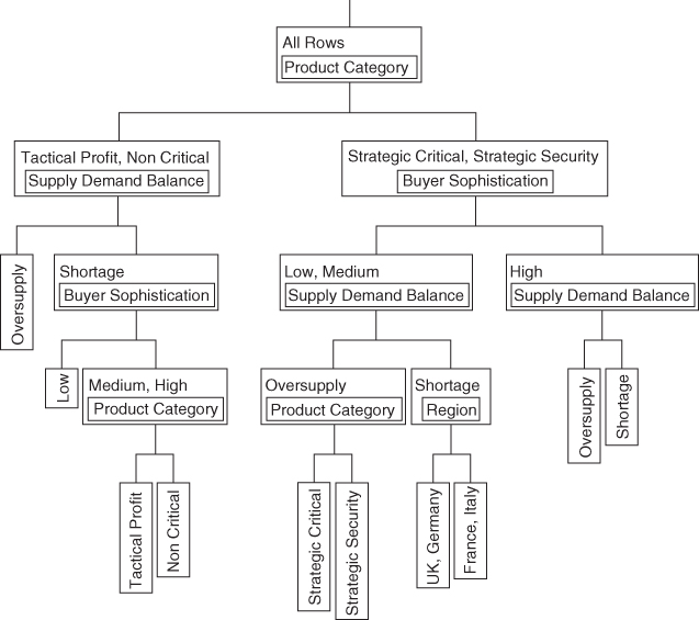
Exhibit 6.22 Small Tree View after Nine Splits
To better understand the split on Region, navigate to that split in your large tree (see Exhibit 6.23). The split on Region is a split of the 72 records that fall into the Supply Demand Balance(Shortage) node at this point in the tree (note that there are three splits on Supply Demand Balance). The Supply Demand Balance(Shortage) node contains relatively few records (2.78 percent) reflecting defective sales. The further split into the two groupings of regions attempts to explain the Yes values, using the fact that there are no defective sales in France or Italy at that point in the tree. But the proportions of Yes values in the two nodes are not very different (0.06 and 0.00).

Exhibit 6.23 Nodes Relating to Split on Region
You do not see this as useful information. You suspect this was one of the last splits. Click the Prune button once. Looking at the Small Tree View, you see that this split has been removed, indicating that it was indeed the ninth split. You are content to proceed with your analysis based on the tree with eight splits. The script for this analysis is Partition—Eight Splits.
Partition Conclusions
Studying your large tree, you see evidence of several local interactions. For example, Exhibit 6.24 shows that for Tactical Profit and Non Critical products, Buyer Sophistication explains variation in times of Shortage but not necessarily in times of Oversupply, with the Low-sophistication buyers resulting in substantially fewer defects (66.67 percent) than High- and Medium-sophistication buyers (96.25). Again the message surfaces that sales representatives need to know how to negotiate with sophisticated buyers.

Exhibit 6.24 Example of a Local Interaction
You can obtain a summary of all the terminal nodes by selecting Leaf Report from the red triangle menu at the top of the report. The resulting Leaf Report describes all nine terminal nodes and gives their response probabilities (proportions) and counts. See Exhibit 6.25.

Exhibit 6.25 Leaf Report
You would like to see the listing of the node descriptions in decreasing order of proportion defective, in other words, with the proportions under the Yes heading in the Response Prob table listed in descending order.
Study both the Leaf Report and the large tree carefully to arrive at these conclusions:
Product Categoryis the key determining factor for pricing defects. Pricing defects are generally less likely with Strategic Critical or Strategic Security products. However, with High-sophistication buyers, a high defective rate can result even for these products, both in Oversupply (93.48 percent) and Shortage (69.57 percent) situations.Buyer Sophisticationinteracts in essential ways withProduct CategoryandSupply Demand Balance. The general message is that for Strategic Critical and Strategic Security sales, pricing defects are much more likely with buyers of High sophistication (81.52 percent) than for those with Low and Medium sophistication (29.86 percent). In periods of Shortage, sales of these products to Low- and Medium-sophistication buyers result in very few defects (2.78 percent), but sales to High-sophistication buyers have a high defective rate (69.57 percent).Supply Demand Balancealso interacts in a complex way withProduct CategoryandBuyer Sophistication. The general message is that for Strategic Critical and Strategic Security sales involving Low- and Medium-sophistication buyers, pricing defects are less likely when there is a Shortage rather than an Oversupply.
When you review this analysis with the team, your team members concur that these conclusions make sense to them. Their lively discussion supports the suggestion that sales representatives are not equipped with tools to deal effectively with sophisticated buyers. Team members believe that sophisticated buyers exploit their power in the negotiation much more effectively than do the sellers. In fact, regardless of buyer sophistication, sales representatives may not know how to exploit their negotiating strength to its fullest potential in times of oversupply.
Also, the experiences of the team members are consistent with the partition analysis' conclusion that the only occasions when sales representatives are almost guaranteed to achieve at least a 5 percent price increase is when they are selling products for which buyers have few other options for purchase (Strategic Critical and Strategic Security) and dealing with less sophisticated buyers (Low and Medium) in times of product shortage. However, the team members do express some surprise that Sales Rep Experience did not surface as a factor of interest.
At this point, you take stock of where you are relative to the Visual Six Sigma Data Analysis Process (Exhibit 6.27). You have successfully completed the Uncover Relationships step, having performed some fine detective work in uncovering actionable relationships among the Xs and Ys. Although all of your work to this point has been exploratory, given the amount of corroboration of your exploratory results by team members who know the sales area intimately, you feel that you could skip the Model Relationships step and move directly to the Revise Knowledge step. This would have the advantage of keeping your analysis lean. But you reflect that your data set is not large. So a quick modeling step using traditional confirmatory analysis might be good insurance. You proceed to undertake this analysis.

Exhibit 6.27 Visual Six Sigma Data Analysis Process
MODELING RELATIONSHIPS
For a traditional confirmatory analysis, you need to use an analysis method that permits hypothesis testing. You could use logistic regression, with Defective as your nominal response. However, the partition analysis provided a good examination of this response and, besides, the continuous variable % Price Increase should be more informative. For this reason, you decide to model % Price Increase as a function of the Xs using Fit Model.
But which Xs should you include? And what about interactions, which the partition analysis clearly indicated were of importance? Fit Model fits a multiple linear regression. You realize that for a regression model, nominal variables with too many values can cause issues relative to estimating model coefficients. So you need to be selective relative to which nominal variables to include. In particular, there is no reason to include Customer ID or Sales Rep, as these variables would not easily help you address root causes even if they were significant.
Now, Region is an interesting variable. There could well be interactions between Region and the other Xs, but you are not sure these would be helpful in addressing root causes. The sales representatives need to be able to sell in all regions. You decide to include Region in the model to verify whether there is a Region effect (your exploratory work has suggested that there is not), but not to include any interactions with Region. You will include all other interactions in your model.
Click Run to fit the model. The report in Exhibit 6.29 appears. (The script is Fit Model—% Price Increase.) The Actual by Predicted plot shows that the data appear randomly spread about the solid line that describes the model. There are no apparent patterns or outliers. (We will not delve into the details of residual analysis or, more generally, multiple regression at this time; there are many good texts that cover this topic.) You conclude that the model provides a reasonable fit to the data.

Exhibit 6.29 Fit Least Squares Report
The Analysis of Variance table shows a Prob > F value that is less than 0.0001. This indicates that the model successfully explains variability in the response.
The Effect Summary report at the top lists the model effects and gives p-values (PValue column) for each. The effects are listed in order of increasing p-values. This places the most significant effects closest to the top. You will consider any effect with a p-value less than or equal to 0.05 to be significant. The significant effects are:
Product CategoryBuyer SophisticationBuyer Sophistication*Product CategorySupply Demand BalanceSales Rep Experience*Product Category
What is very interesting is that Sales Rep Experience has appeared in the list. On its own, it is not significant, but it is influential through its interaction with Product Category. This is an insight that did not appear in your exploratory analyses. In fact, your exploratory results led you to believe that Sales Rep Experience did not have an impact on defective sales negotiations. But you need to keep in mind that your multivariate exploratory technique, partition analysis, used a nominal version of the response. Nominal variables tend to carry less information than do their continuous counterparts. Also, partition and multiple linear regression are very different techniques. These two comments may offer an explanation of why this interaction was not seen earlier, which in turn reinforces the need to use complementary approaches to analysis rather than simply relying on one method in isolation.
These two plots show the means predicted by the model (Exhibit 6.30).

Exhibit 6.30 LSMeans Plot for Two Significant Interactions
From the first plot, you conclude that there is some evidence that High-experience sales representatives tend to get slightly higher price increases than do Medium- and Low-experience sales representatives for Strategic Security products. (Open the Least Squares Means Table to see that they average about 0.8 percent more.) You wonder, “Do they know something that could be shared?”
In the second plot, you see the effect of High-sophistication buyers—they negotiate lower price increases across all categories, but especially for Strategic Security products (about 3 percent lower than do Low- or Medium-sophistication buyers for those products). For Tactical Profit products, Medium-sophistication buyers get lower price increases than do Low-sophistication buyers. For other product categories, there is little difference between Medium- and Low-sophistication buyers. Clearly, there would be much to gain by addressing High-sophistication buyers, especially when dealing with Strategic Security products.
These findings are consistent with and extend the conclusions that you drew earlier from your exploratory analyses. You are ready to move on to addressing the problem of too many pricing defects.
REVISING KNOWLEDGE
At this point, you are confident that you have identified a number of Hot Xs. You are ready to move on to the Revise Knowledge step of the Visual Six Sigma Data Analysis Process.
To find conditions that will optimize the pricing process, as well as to ensure that no significant Xs have been overlooked, you involve your team members and a larger group of sales representatives in discussing your observations and conclusions and in suggesting ways to improve the pricing process. After all, the sales representatives are the ones working with the pricing management process on a daily basis, and you know that their knowledge and support will be critical when you move into the imminent improvement phase of this project.
Once this is accomplished, you will meet with Bill to formulate an improvement plan. You intend to monitor pricing over a short pilot period in a limited market segment to verify that the improvement plan will lead to sustainable benefits before changes are institutionalized.
Identifying Optimal Strategies
You organize a number of workshops where you present the findings of your data analysis. You are delighted and even surprised by the enthusiastic feedback that you receive. Typical comments are:
- “I really like what you showed me…. It's simple to understand and tells a really clear story.”
- “I've been frustrated for a while. Now at last I can see what is going on.”
- “At last—someone prepared to listen to us—we've been saying for some time that we need sales managers to understand some of our problems.”
- “It really looks like we are being out-negotiated. If we focus on our strengths and exploit the great products we have, then I'm sure we can win.”
- “We've allowed our competition to drive prices down for too long. We need to do something quickly, and this gives us some really good ideas.”
Specifically, the sales representatives highlight:
- The need for more training in negotiation skills.
- The need for more realistic sales management guidelines and price targets through a tailored price management process. A target 5 percent price increase across the board is seen by them as a very blunt instrument. They want a more finely tuned approach that aims for higher increases where Polymat has strong competitive advantage (as in the Strategic Security and Strategic Critical product categories), but lower target increases in commodity areas (as in the Tactical Profit product category). They strongly feel that this would allow them to focus their time and negotiating energy where the return on their investment is the highest.
You capture all the Xs that might lead to effective price increases, both from your analyses and ideas generated by the sales representatives, in a cause-and-effect diagram (Exhibit 6.31). You construct the cause-and-effect diagram in JMP, using Analyze > Quality and Process > Diagram.

Exhibit 6.31 Cause-and-Effect Diagram for Price Increase
Using boldface, italicized text, you highlight potential causes that are identified as important based on your data analysis and the sales representatives' discussions. The data are in the table CauseAndEffectTable.jmp and the script is Cause-and-Effect Diagram.
We encourage you to consult the Help files to see how the cause-and-effect diagram is constructed: Go to Help > Books > Quality and Process Methods and find the chapter called “Cause-and-Effect Diagrams.”
You now consolidate your findings for a summary meeting with Bill. You summarize the Xs identified from a combination of the data analysis and the sales representatives' input in an Impact and Control Matrix, shown in Exhibit 6.32. From your experience, you find this to be a powerful tool for crystallizing findings and directing an improvement strategy.

Exhibit 6.32 Impact and Control Matrix
The Impact axis is the relative size of the impact that an X has on overall process performance. For those Xs for which you have quantitative information, you use this information to help make decisions on their degree of impact. However, for Xs where you have only qualitative information from the sales representatives, this assignment is necessarily more subjective.
The Control axis relates to the degree of control or influence that can be exercised on this X through process redesign. Environmental factors, such as Buyer Sophistication, are not things that can be influenced (absent unethical business practices)—sales representatives have to deal with the buyers who are facing them in the negotiation. However, the training of sales representatives, such as the type of training, frequency of training, and appropriateness of training, is within the control of Polymat.
You decide to place Supply Demand Balance in the Medium Control category despite its appearance as an environmental factor outside Polymat's control. The reasoning behind this is that although Supply Demand Balance itself cannot be directly controlled, Polymat's leadership team can control the timing of any price increase in response to market conditions. You believe that this timing could be better managed to ensure that price increases are only attempted when the overall supply/demand balance is favorable, such as in periods of relative shortage.
The Xs toward the top right of the Impact and Control Matrix are clearly the ones on which you and your team should focus in the Improve phase of DMAIC. These Xs have a big impact and can be strongly influenced or controlled by better process design.
Improvement Plan
After his sponsor review meeting with you and your team, Bill is delighted. “I told you that I thought we were leaving money on the table in our pricing negotiations. Now, thanks to your fine work, I have the analysis that really convinces me!”
Moreover, Bill is extremely enthusiastic about the visual capabilities of JMP. He admits privately to you that he was concerned that he might not be able to convince his colleagues of the need to adopt a Six Sigma approach. His colleagues are not very process-oriented and have little time for what they view as the “statistical complexity of the Six Sigma approach.” Bill can see that by using Visual Six Sigma he is able to tell a simple but compelling story that shows a clear direction for Polymat's pricing efforts.
With your help and input, Bill pulls together an improvement plan focusing on four key areas:
- Product Category. The analysis has illustrated the power of your product categorization method for Polymat. Because this work used only sample products and customers, Bill agrees to convene workshops to classify all of the significant products in Polymat's portfolio in this way. You work with Bill to develop a review process to keep this classification current.
-
Sales Representative Training. The analysis highlighted the relative weakness of sales representatives in the price negotiation process. Sophisticated buyers are much more successful in keeping prices low than are sales representatives in negotiating prices up. This was reinforced by the sales representatives themselves, who requested more training in this area.
Consequently, Bill agrees to focused training sessions to improve negotiation skills. These are to be directly linked to the new product categorization matrix to ensure that sales representatives fully exploit the negotiating strength provided by Polymat's Strategic Critical and Strategic Security products.
-
New Rules for Supply/Demand Balance Decisions. Recognizing the need to understand the prevailing supply/demand balance before adjusting pricing targets, Bill allocates one of his senior market managers to join your team.
His role is to develop a monitoring process using trade association data to track market dynamics by quarter. This process will be designed to take account of fluctuations in demand and also to track imports, exports, and the startup of new suppliers. Business rules will flag when price increases are likely to be successful, and Polymat's leadership team will trigger the price management process to make an appropriate response.
- Price Management Process Redesign. Bill agrees that a total reengineering of the price management process is needed. You and Bill set up a workshop to begin the process redesign, and, during an intensive two-day offsite meeting, the workshop team develops a redesign with the following features:
- Step 1. Based on a target-setting worksheet, Polymat sales managers will review each key customer and product combination and agree to the percent price increase target for that particular product at that customer. This replaces the blanket 5 percent increase that has been used up to now. Typically, the targeted increase will be in the range of 0–10 percent.
- Step 2. Using the worksheet, price negotiations will be tracked at weekly account reviews. The current status will be flagged using red-yellow-green traffic signals, so that sales managers can support the sales representatives' negotiations as needed.
- Step 3. At the agreed date of the price increases, the newly mandated price targets are input into the order entry system for subsequent transactions.
- Step 4. Following the price increases, the actual invoiced prices will be downloaded from the order entry system and checked against the new target. Any remaining pricing defects can then be remediated as necessary. A dashboard of summary reports will allow the Polymat business leadership team to track planned versus actual performance.
The leadership team agrees to take a phased approach to implementing the new process design, starting with a six-month pilot in one market segment. Unfortunately, the market seems to be switching from Oversupply to Shortage just as the pilot starts.
Verifying Improvement
About six months later, you sit down with Bill to review some new data. The market did switch from Oversupply to Shortage, so this data reflects a Supply Demand Balance period of Shortage.
Your new data table is called PilotPricing.jmp. It consists of data on all of the product and company combinations used in the previous study that had activity during the pilot period. Over the period of the pilot study, only three companies did not purchase the product that they had purchased during the baseline study. Consequently, the data table consists of 237 rows.
You are interested in comparing the current level of % Price Increase with your baseline. However, since Polymat is in a Supply Demand Balance period of Shortage, you need to compare you pilot study data with baseline data for Shortage periods.
The new pricing management process has delivered a mean price increase of about 5.8 percent.
You would like to see the histograms for % Price Increase during the pilot period and for % Price Increase during the baseline period of Shortage next to each other. You also want the histograms plotted with the same axis settings to facilitate comparing the two histograms.
Exhibit 6.33 shows the Distribution report for the pilot period (top plot) and the Distribution report for the baseline period when Supply Demand Balance is Shortage (bottom plot).

Exhibit 6.33 Distribution Reports for % Price Increase during Pilot Study and during Baseline Shortage Period
The improvement is obvious. The % Price Increase histogram for the pilot period (top, in Exhibit 6.33) is shifted to the right of the histogram for the baseline in the period of shortage. The mean increase in the pilot period is 5.8 percent, compared with a mean increase of 4.7 percent for the baseline data when there was a supply shortage. Although an approximate 1 percent gain in % Price Increase does not appear dramatic, you calculate that for the complete Polymat portfolio this is worth in excess of 2 million British pounds per year.
Next you delve a little more deeply into the data to see the nature of underlying changes. You are particularly interested in your Hot Xs and how they relate to % Price Increase.
You explore the data by clicking on bars in the graphs, just as you did when exploring the baseline data. You are intrigued by the following: In the Product Category bar plot, when you shift-click on the Strategic Security and Strategic Critical bars, you see a noticeable impact on % Price Increase (Exhibit 6.34).

Exhibit 6.34 Distribution Report Showing Product Category Impact
You would like to compare the mean % Price Increase for these two categories to the % Price Increase during the baseline period of shortage.
The mean % Price Increase for these two categories during the pilot period is 8.12 percent. You go back to your BaselinePricing.jmp data table and conduct a similar analysis using the Local Data Filter. This analysis shows that for the baseline data, in the Shortage period, the % Price Increase for these two categories was only 5.88 percent.
You remind Bill that, for these product categories, sales representatives have a relatively strong negotiating position due to the small number of alternative options available to the buyer. After the improvements were put in place, the price increase for these products is strongly skewed to markedly higher levels, suggesting much more effective and targeted negotiations during the pilot period.
You want to further study the impact of Product Category and Buyer Sophistication on % Price Increase over the pilot period.
The report shown in Exhibit 6.37 appears. The comparison circles (and associated tests) show no evidence of a Buyer Sophistication effect on % Price Increase. As expected, though, the Product Category effect is present. The means for all four categories are given in this report: Strategic Security and Strategic Critical sales average an increase of 7.68 percent and 8.37 percent respectively while the other two categories average increases of 4.87 percent and 2.64 percent.

Exhibit 6.37 Oneway Reports for % Price Increase
You take the data, these reports, and a summary of your key findings from the pilot to a review meeting with Bill and the Polymat leadership team. Convinced by this study, the leadership team immediately gives the go-ahead to implement the new pricing management process as rapidly as possible across all operations.
UTILIZING KNOWLEDGE: SUSTAINING THE BENEFITS
Your pricing project was initiated by Bill in response to frustration over a consistent Polymat price decline during an extended period due to:
- Increasing commoditization of products
- Increasing competition from low-cost, Far Eastern suppliers
Bill had a hunch that sales representatives were weak in pricing negotiations, and you were able to clearly show that this was the case. You were also able to target specific areas where those negotiation skills could be improved. Exploiting the insights from a Visual Six Sigma analysis of failed attempts to increase price unilaterally, you adapted and promoted a practical and simple tool that was better able to capture the value proposition of products to customers.
Using this tool allowed sales representatives to become better prepared for specific price negotiations and to receive support if necessary. The pricing management process was redesigned as an ongoing, data-driven, business process to be triggered periodically when market or business conditions were deemed conducive to price changes. The results from the pilot indicate yearly revenue increases on the order of 2 million British pounds for Polymat's current operations.
In line with the price management process redesign, Bill now wants a monitoring mechanism that allows the Polymat leadership team to easily track what is happening to their prices over time, picking up early shifts and patterns that might give another means to trigger their pricing review activity. So, as the final step in the project, you are asked to provide Bill with a simple way to visually track shifts and trends in Polymat's prices, ideally using leading rather than lagging indicators, so that Polymat can react appropriately.
To do this, you draw inspiration from the idea of the Retail Price Index. You create a Polymat Price Index based on a collection of Polymat products. This index is based on the price of a fixed volume of these selected products and is corrected for currency exchange fluctuations and inflation. It will be monitored quarterly by the leadership team. The leadership team hopes to see the Polymat Price Index rise over time.
You write a JMP script to calculate the Polymat Price Index by quarter. You calculate the index by quarter for the year preceding the pilot and for the pilot period itself. The data are given in PriceIndex1.jmp. Your plan is to monitor this Price Index using an individual measurement chart.
The resulting chart is shown in Exhibit 6.38. The upper and lower horizontal lines shown here for each level of Stage are control limits (they appear red on a computer screen). You are somewhat disappointed because, although there may be a trend forming over the project period, there is no statistical evidence that that trend is anything more than random variation. Still the index has increased relative to the Historical period. However, the early part of the Historical period saw oversupply and that might explain the lower values. You realize that it may take time for the improvements to reveal themselves.

Exhibit 6.38 Control Chart for Polymat Price Index over Historical and Pilot Periods
You continue to update your chart with quarterly data over the next three years. Now you are able to calculate the Polymat Price Index over three Stage periods:
- Historical—the year prior to the initiation of the project
- Project—the year during which the project was conducted and tested
- Post-Project—the three subsequent years
The data table containing your data is PriceIndex2.jmp. You construct a three-phase control chart using instructions identical to those used to construct the control chart in Exhibit 6.38. The control chart is shown in Exhibit 6.39 and data table script is Control Chart Builder.

Exhibit 6.39 Control Chart for Polymat Price Index over Five Years
Bill and the Polymat management team realize that control charts, such as Exhibit 6.39, are powerful tools for tracking long-term trends in Polymat pricing. Clearly the improvement work is having an impact in halting and reversing the historical downward trend. Once the process stabilizes, control limits based on that stable period can be used as objective decision limits to flag changes in pricing.
CONCLUSION
This case study illustrates how Visual Six Sigma can be exploited beyond the traditional data-driven manufacturing and engineering areas. Almost any business involved in selling products or services generates data in their transactional activities, but such data are often used exclusively for accounting, rather than for improvement. In process terms, pricing and price management generally remain something of an art.
Pricing data are a very rich source of information about dynamics of the market and the relationship between suppliers and their customers. In our case study, using Visual Six Sigma reveals some dramatic insights. In response to these findings, a simple and pragmatic value analysis tool is developed to help sales representatives focus their price negotiations more effectively. In addition, new measurement tools are developed that enable the supplier to better align its price adjustments with shifts in market conditions.
Using Visual Six Sigma, the messages that were contained in Polymat's historical price change data revealed themselves as clear and unambiguous. These findings could be presented in ways that were not clouded in statistical language and that told a compelling story leading quickly to improvement opportunities. Although access to subject matter expertise was vital, Visual Six Sigma allowed you to make rapid progress with only the need for periodic consultations with other Polymat personnel.
These findings led to the development of simple but powerful approaches founded on measurements that were easily implemented. The sales representatives, sales managers, and Polymat's leadership team readily adopted these approaches because they were practical, gave new insights, and delivered visible and measurable benefits.