Overview
This chapter introduces the concept of regularization for neural networks. Regularization aims to prevent the model from overfitting the training data during the training process and provides more accurate results when the model is tested on new unseen data. You will learn to utilize different regularization techniques—L1 and L2 regularization and dropout regularization—to improve model performance. Regularization is an important component as it prevents neural networks from overfitting the training data and helps us build robust, accurate models that perform well on new, unseen data. By the end of this chapter, you will be able to implement a grid search and random search in scikit-learn and find the optimal hyperparameters.
Introduction
In the previous chapter, we continued to develop our knowledge of creating accurate models with neural networks by experimenting with cross-validation as a method to test how various hyperparameters perform in an unbiased manner. We utilized leave-one-out cross-validation, in which we leave one record out of the training process for use in validation and repeat this for every record in the dataset. Then, we looked at k-fold cross-validation, in which we split the training dataset into k folds, train the model on k-1 folds, and use the final fold for validation. These cross-validation methods allow us to train models with different hyperparameters and test their performance on unbiased data.
Deep learning is not only about building neural networks, training them using an available dataset, and reporting the model accuracy. It involves trying to understand your model and the dataset, as well as moving beyond a basic model by improving it in many aspects. In this chapter, you will learn about two very important groups of techniques for improving machine learning models in general, and deep learning models in particular. These techniques are regularization methods and hyperparameter tuning.
This chapter will further cover regularization methods—specifically, why we need them and how they help. Then, we'll introduce two of the most important and most commonly used regularization techniques. Here, you'll learn about parameter regularization and its two variations, L1 and L2 norm regularizations, in great detail. You will then learn about a regularization technique that was specifically designed for neural networks called dropout regulation. You will also practice implementing each of these techniques on Keras models by completing activities that involve real-life datasets. We'll end our discussion of regularization by briefly introducing some other regularization techniques that you may find helpful later in your work.
Then, we will talk about the importance of hyperparameter tuning, especially for deep learning models, by exploring how tuning the values of hyperparameters can dramatically affect model accuracy, as well as the challenge of tuning the many hyperparameters that require it when building deep neural networks. You will learn two very helpful methods in scikit-learn that you can use for performing hyperparameter tuning on Keras models, the benefits and drawbacks of each method, and how to combine them to gain the most from both. Lastly, you will practice implementing hyperparameter tuning for Keras models using scikit-learn optimizers by completing an activity.
Regularization
Since deep neural networks are highly flexible models, overfitting is an issue that can often arise when training them. Therefore, one very important part of becoming a deep learning expert is knowing how to detect overfitting, and subsequently how to address the overfitting problem in your model. Overfitting in your models will be clear if your model performs excellently on the training data but performs poorly on new, unseen data.
For example, if you build a model to classify images of dogs and cats into their respective classes and your image classifier performs with high accuracy during the training process but does not perform well on new examples, then this is an indication that your model has overfitted the training data. Regularization techniques are an important group of methods specifically aimed at reducing overfitting in machine learning models.
Understanding regularization techniques thoroughly and being able to apply them to your deep neural networks is an essential step toward building deep neural networks in order to solve real-life problems. In this section, you will learn about the underlying concepts of regularization, which will provide you with the foundation that's required for the following sections, where you will learn how to implement various types of regularization methods using Keras.
The Need for Regularization
The main goal of machine learning is to build models that perform well, not only on the examples they are trained on but also on new examples that were not included in the training. A good machine learning model is one that finds the form and the parameters of the true underlying process/function that's producing the training examples but does not capture the noise associated with individual training examples. Such a machine learning model can generalize well to new data that's produced by the same process later.
The approaches we discussed previously—such as splitting a dataset into a training set and a test set, and cross-validation—were all designed to estimate the generalization ability of a trained model. In fact, the term that's used to refer to a test set error and cross-validation error is "generalization error." This simply means the error rate on examples that were not used in training. Once again, the main goal of machine learning is to build models with low generalization error rates.
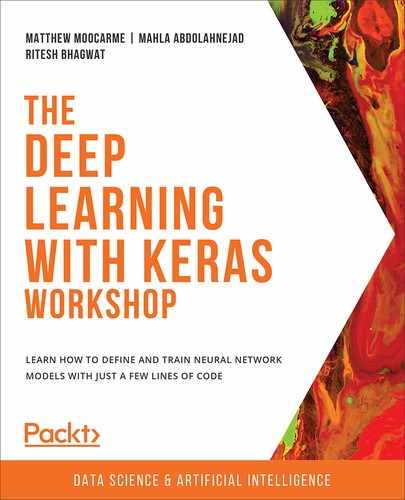
In Chapter 3, Deep Learning with Keras, we discussed two very important issues with machine learning models: overfitting and underfitting. We stated that underfitting is the scenario where the estimated model is not flexible or complex enough to capture all the relations and patterns associated with the true process. This is a model with high bias and is detected when the training error is high. On the other hand, overfitting is the scenario where the model that's used for estimating the true process is too flexible or complex. This is a model with high variance and is diagnosed when there is a large gap between the training error and the generalization error. An overview of these scenarios for a binary classification problem can be seen in the following images:

Figure 5.1: Underfitting
As you can see above, Underfitting is a less problematic issue than overfitting. In fact, underfitting can be fixed easily by making the model more flexible/complex. In deep neural networks, this means changing the architecture of the network, making the network larger by adding more layers to it or increasing the number of units in the layers.
Now let's look at overfitting image below:

Figure 5.2: Overfitting
Similarly, there are simple solutions for addressing overfitting, such as making the model less flexible/complex (again, by changing the architecture of the network) or providing the network with more training examples. However, making the network less complex sometimes comes at the cost of a dramatic increase in bias or training error rate. The reason for this is that most of the time, the cause of overfitting is not the flexibility of the model but too few training examples. On the other hand, providing more data examples in order to decrease overfitting is not always possible. As a result, finding ways to reduce the generalization error while keeping model complexity and the number of training examples fixed is both important and challenging.
Now let's look at the Right fit image below:
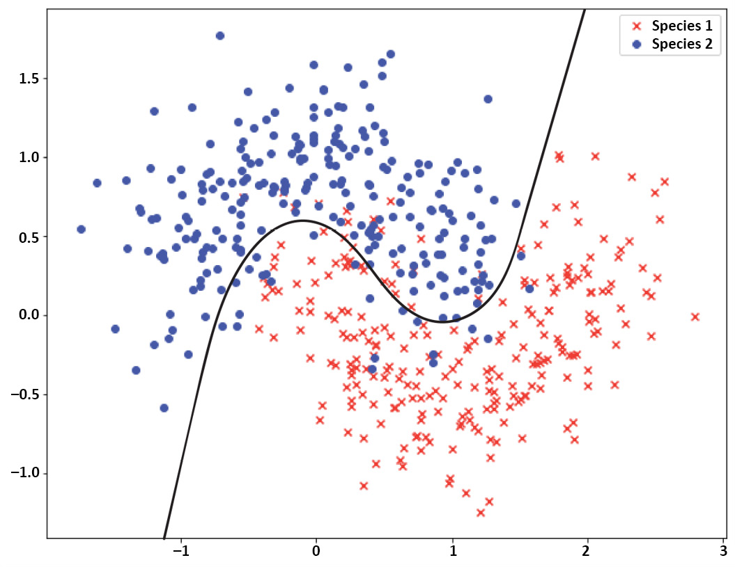
Figure 5.3: Right Fit
That is why we need regularization techniques when building highly flexible machine learning models, such as deep neural networks, to suppress the flexibility of the model so that it cannot overfit to individual examples. In the next section, we will describe how regularization methods reduce the overfitting of models on the training data to reduce the variance in the model.
Reducing Overfitting with Regularization
Regularization methods try to modify the learning algorithm in a way that reduces the variance of the model. By decreasing the variance, regularization techniques intend to reduce the generalization error while not increasing the training error (or, at least, not increasing the training error drastically).
Regularization methods provide some kind of restriction that helps with the stability of the model. There are several ways that this can be achieved. One of the most common ways of performing regularization on deep neural networks is by putting some type of penalizing term on weights to keep the weights small.
Keeping the weights small makes the network less sensitive to noise in individual data examples. Weights in a neural network are, in fact, the coefficients that determine how big or small an effect each processing unit will have on the final output of the network. If the units have large weights, it means that each of them will have a significant influence on the output. Combining all the large influences that are caused by each processing unit will result in many fluctuations in the final output.
On the other hand, keeping the weights small reduces the amount of influence each unit will have on the final output. Indeed, by keeping the weights near zero, some of the units will have almost no effect on the output. Training a large neural network where each unit has little or no effect on the output is the equivalent of training a much simpler network, and so variance and overfitting are reduced. The following figure shows the schematic view of how regularization zeroes out the effect of some units in a large network:

Figure 5.4: Schematic view of how regularization zeroes out the effect of some units in a large network
The preceding diagram is a schematic view of the regularization process. The top network shows a network without regularization, while the bottom network shows an example of a network with regularization in which the white units represent units that have little to no effect on the output because they have been penalized by the regularization process.
So far, we have learned about the concepts behind regularization. In the next section, we will look at the most common methods of regularization for deep learning models—L1, L2, and dropout regularization—along with how to implement them in Keras.
L1 and L2 Regularization
The most common type of regularization for deep learning models is the one that keeps the weights of the network small. This type of regularization is called weight regularization and has two different variations: L2 regularization and L1 regularization. In this section, you will learn about these regularization methods in detail, along with how to implement them in Keras. Additionally, you will practice applying them to real-life problems and observe how they can improve the performance of a model.
L1 and L2 Regularization Formulation
In weight regularization, a penalizing term is added to the loss function. This term is either the L2 norm (the sum of the squared values) of the weights or the L1 norm (the sum of the absolute values) of the weights. If the L1 norm is used, then it will be called L1 regularization. If the L2 norm is used, then it will be called L2 regularization. In each case, the sum is multiplied by a hyperparameter called a regularization parameter (lambda).
Therefore, for L1 regularization, the formula is as follows:
Loss function = Old loss function + lambda * sum of absolute values of the weights
And for L2 regularization, the formula is as follows:
Loss function = Old loss function + lambda * sum of squared values of the weights
Lambda can take any value between 0 and 1, where lambda=0 means no penalty at all (equivalent to a network with no regularization) and lambda=1 means full penalty.
Like every other hyperparameter, the right value for lambda can be selected by trying out different values and observing which value provides a lower generalization error. In fact, it's good practice to start with a network with no regularization and observe the results. Then, you should perform regularization with increasing values of lambda, such as 0.001, 0.01, 0.1, 0.5, …, and observe the results in each case in order to figure out how much penalizing on the weight's values is suitable for a particular problem.
In each iteration of the optimization algorithm with regularization, the weights (w) become smaller and smaller. That is why weight regularization is commonly referred to as weight decay.
So far, we have only discussed regularizing weights in a deep neural network. However, you need to keep in mind that the same procedure can be applied to biases as well. More precisely, we can update the loss function again by adding a bias penalizing term to it as well and therefore keep the values of biases small during the training of a neural network.
Note
If you perform regularization by adding two terms to the loss function (one for penalizing weights and one for penalizing biases), then we call it parameter regularization instead of weight regularization.
However, regularizing bias values is not very common in deep learning. The reason for this is that weights are much more important parameters of neural networks. In fact, usually, adding another term to regularize biases will not change the results dramatically in comparison to only regularizing the weight values.
L2 regularization is the most common regularization technique that's used in machine learning in general. The difference between L1 regularization and L2 regularization is that L1 results in a sparser weights matrix, meaning there are more weights equal to zero, and therefore more nodes that are completely removed from the network. L2 regularization, on the other hand, is more subtle. It decreases the weights drastically, but at the same time leaves you with fewer weights equal to 0. It is also possible to perform both L1 and L2 regularization at the same time.
Now that you have learned about how L1 and L2 regularization work, you are ready to move on to implementing L1 and L2 regularization on deep neural networks in Keras.
L1 and L2 Regularization Implementation in Keras
Keras provides a regularization API that can be used to add penalizing terms to the loss function in order to regularize weights or biases in each layer of a deep neural network. To define the penalty term or regularizer, you need to define the desired regularization method under keras.regularizers.
For example, to define an L1 regularizer with lambda=0.01, you can write this:
from keras.regularizers import l1
keras.regularizers.l1(0.01)
Similarly, to define an L2 regularizer with lambda=0.01, you can write this:
from keras.regularizers import l2
keras.regularizers.l2(0.01)
Finally, to define both L1 and L2 regularizers with lambda=0.01, you can write this:
from keras.regularizers import l1_l2
keras.regularizers.l1_l2(l1=0.01, l2=0.01)
Each of these regularizers can be applied to weights and/or biases in a layer. For example, if we would like to apply L2 regularization (with lambda=0.01) on both the weights and biases of a dense layer with eight nodes, we can write this:
from keras.layers import Dense
from keras.regularizers import l2
model.add(Dense(8, kernel_regularizer=l2(0.01),
bias_regularizer=l2(0.01)))
We will practice implementing L1 and L2 regularization further in Activity 5.01, Weight Regularization on an Avila Pattern Classifier, in which you will apply regularization on the deep learning model for the diabetes dataset and observe how the results change in comparison to previous activities.
Note
All the activities in this chapter will be developed in Jupyter Notebooks. Please download this book's GitHub repository, along with all the prepared templates, from https://packt.live/2OOBjqq.
Activity 5.01: Weight Regularization on an Avila Pattern Classifier
The Avila dataset has been extracted from 800 images of the Avila Bible, a giant 12th-century Latin copy of the Bible. The dataset consists of various features about the images of the text, such as intercolumnar distance and the margins of the text. The dataset also contains a class label that indicates if a pattern of the image falls into the most frequently occurring category or not. In this activity, you will build a Keras model to perform classification on this dataset according to given network architecture and hyperparameter values. The goal is to apply different types of weight regularization on the model and observe how each type changes the result.
In this activity, we will use the training set/test set approach to perform the evaluation for two reasons. First, since we are going to try several different regularizers, performing cross-validation will take a long time. Second, we would like to plot the trends in the training error and the test error in order to understand, in a visual way, how regularization prevents the model from overfitting to data examples.
Follow these steps to complete this activity:
- Load the dataset from the data subfolder of Chapter05 from GitHub using X = pd.read_csv('../data/avila-tr_feats.csv') and y = pd.read_csv('../data/avila-tr_target.csv'). Split the dataset into a training set and a test set using the sklearn.model_selection.train_test_split method. Hold back 20% of the data examples for the test set.
- Define a Keras model with three hidden layers, the first of size 10, the second of size 6, and the third of size 4, to perform the classification. Use these values for the hyperparameters: activation='relu', loss='binary_crossentropy', optimizer='sgd', metrics=['accuracy'], batch_size=20, epochs=100, and shuffle=False.
- Train the model on the training set and evaluate it with the test set. Store the training loss and test loss at every iteration. After training is complete, plot the trends in training error and test error (change the limits of the vertical axis to (0, 1) so that you can observe the changes in losses better). What is the minimum error rate on the test set?
- Add L2 regularizers with lambda=0.01 to the hidden layers of your model and repeat the training. After training is complete, plot the trends in training error and test error. What is the minimum error rate on the test set?
- Repeat the previous step for lambda=0.1 and lambda=0.005, train the model for each value of lambda, and report the results. Which value of lambda is a better choice for performing L2 regularization on this deep learning model and this dataset?
- Repeat the previous step, this time with L1 regularizers for lambda=0.01 and lambda=0.005, train the model for each value of lambda, and report the results. Which value of lambda is a better choice for performing L1 regularization on this deep learning model and this dataset?
- Add L1_L2 regularizers with the L1 lambda=0.005 and the L2 lambda=0.005 to the hidden layers of your model and repeat the training. After training is complete, plot the trends in training error and test error. What is the minimum error rate on the test set?
After implementing these steps, you should get the following expected output:

Figure 5.5: A plot of the training error and validation error during training for the model with L1 lambda equal to 0.005 and L2 lambda equal to 0.005
Note
The solution for this activity can be found on page 398.
In this activity, you practiced implementing L1 and L2 weight regularizations for a real-life problem and compared the results of the regularized model with those of a model without any regularization. In the next section, we will explore the regulation of a different technique, known as dropout regularization.
Dropout Regularization
In this section, you will learn how dropout regularization works, how it helps with reducing overfitting, and how to implement it using Keras. Lastly, you will practice what you have learned about dropout by completing an activity involving a real-life dataset.
Principles of Dropout Regularization
Dropout regularization works by randomly removing nodes from a neural network during training. More precisely, dropout sets up a probability on each node. This probability refers to the chance that the node is included in the training at each iteration of the learning algorithm. Imagine we have a large neural network where a dropout chance of 0.5 is assigned to each node. In such a case, at each iteration, the learning algorithm flips a coin for each node to decide whether that node will be removed from the network or not. An illustration of such a process can be seen in the following diagram:

Figure 5.6: Illustration of removing nodes from a deep neural network using dropout regularization
This process is repeated at each iteration; this means that, at each iteration, randomly selected nodes are removed from the network, which means the parameter-updating process is done on a different smaller network. For example, the network shown at the bottom of the preceding diagram would be used for one iteration of the training only. For the next iteration, some other randomly selected nodes would be crossed out from the top network so the network that results from removing those nodes would be different from the bottom network in the diagram.
When some nodes are chosen to be removed/ignored in an iteration of a learning algorithm, it means that they won't participate in the parameter-updating process at all in that iteration. More precisely, the forward propagation to predict the output, the loss computation, and the backpropagation to compute the derivatives are all to be done on the smaller network with some nodes removed. Consequently, parameter updating will only be done on the nodes that are present in the network in that iteration; the weights and biases of removed nodes won't be updated.
However, it is important to keep in mind that to evaluate the performance of the model on the test set or hold-out set, the original complete network is always used. If we perform the evaluation of a network with random nodes deleted from it, the noise will be introduced to the results, and this is not desirable.
In dropout regularization, training is always performed on the networks that result from randomly selected nodes being removed from the original network. Evaluation is always performed using the original network. In the next section, we will gain an understanding of why dropout regularization helps prevent overfitting.
Reducing Overfitting with Dropout
In this section, we are going to discuss the concepts behind dropout as a regularization method. As we discussed previously, the goal of regularization techniques is to prevent a model from overfitting data. Therefore, we are going to look at how randomly removing a portion of nodes from a neural network helps reduce variance and overfitting.
The most obvious explanation of why removing random nodes from the network prevents overfitting is that by removing nodes from a network, we are performing training on a smaller network in comparison to the original network. As you learned previously, a smaller neural network provides less flexibility, so the chance of the network overfitting to data is lower.
There is another reason why dropout regularization does such a good job of reducing overfitting. By randomly removing inputs at each layer in a deep neural network, the overall network becomes less sensitive to single inputs. We know that, while training a neural network, the weights are updated in a way that the final model will fit to the training examples. By removing some of the weights from the training process at random, dropout forces other weights to participate in learning the patterns related to the training examples at that iteration, and so the final weight values will better spread out more.
In other words, instead of some weights updating too much in order to fit some input values, all the weights learn to participate in learning those input values and, consequently, overfitting decreases. This is why performing dropout results in a much more robust model—performing better on new, unseen data—in comparison to simply using a smaller network. In fact, dropout regularization tends to work better on larger networks.
Now that you have learned all about the underlying procedure of dropout and the reasons behind its effectiveness, we can move on to implementing dropout regularization in Keras.
Exercise 5.01: Dropout Implementation in Keras
Dropout regularization is provided as a core layer in Keras. As such, you can add dropout to your model in the same way that you would add layers to your network. When defining a dropout layer in Keras, you need to provide the rate hyperparameter as an argument. rate can take any value between 0 and 1 and determines the portions of the input units to be removed or ignored. In this exercise, you will learn the step-by-step process of implementing a Keras deep learning model with dropout layers.
Our simulated dataset represents various measurements of trees, such as height, the number of branches, and the girth of the trunk at the base. Our goal is to classify the records into either deciduous (a class value of 1) or coniferous (a class value of 0) type trees based on the measurements given. The dataset consists of 10000 records that consist of two classes, representing the two tree types, and each data example has 10 feature values. Follow these steps to complete this exercise:
- First, execute the following code block to load in the dataset and split the dataset into a training set and a test set:
# Load the data
import pandas as pd
X = pd.read_csv('../data/tree_class_feats.csv')
y = pd.read_csv('../data/tree_class_target.csv')
"""
Split the dataset into training set and test set with a 80-20 ratio
"""
from sklearn.model_selection import train_test_split
seed = 1
X_train, X_test,
y_train, y_test = train_test_split(X, y,
test_size=0.2,
random_state=seed)
- Import all the necessary dependencies. Build a four-layer Keras sequential model without dropout regularization. Build the network with 16 units in the first hidden layer, 12 units in the second hidden layer, 8 units in the third hidden layer, and 4 units in the fourth hidden layer, all with ReLU activation functions. Add an output layer with a sigmoid activation function:
#Define your model
from keras.models import Sequential
from keras.layers import Dense, Activation
import numpy as np
from tensorflow import random
np.random.seed(seed)
random.set_seed(seed)
model_1 = Sequential()
model_1.add(Dense(16, activation='relu', input_dim=10))
model_1.add(Dense(12, activation='relu'))
model_1.add(Dense(8, activation='relu'))
model_1.add(Dense(4, activation='relu'))
model_1.add(Dense(1, activation='sigmoid'))
- Compile the model with binary cross-entropy as the loss function and sgd as the optimizer and train the model for 300 epochs with batch_size=50 on the training set. Then, evaluate the trained model on the test set:
model_1.compile(optimizer='sgd', loss='binary_crossentropy')
# train the model
model_1.fit(X_train, y_train, epochs=300, batch_size=50,
verbose=0, shuffle=False)
# evaluate on test set
print("Test Loss =", model_1.evaluate(X_test, y_test))
Here's the expected output:
2000/2000 [==============================] - 0s 23us/step
Test Loss = 0.1697693831920624
Therefore, the test error rate for predicting the species of tree after training the model for 300 epochs is equal to 16.98%.
- Redefine the model with the same number of layers and same size in each layer as the prior model. However, add a dropout regularization of rate=0.1 to the first hidden layer of your model and repeat the compilation, training, and evaluation steps of the model on the test data:
"""
define the keras model with dropout in the first hidden layer
"""
from keras.layers import Dropout
np.random.seed(seed)
random.set_seed(seed)
model_2 = Sequential()
model_2.add(Dense(16, activation='relu', input_dim=10))
model_2.add(Dropout(0.1))
model_2.add(Dense(12, activation='relu'))
model_2.add(Dense(8, activation='relu'))
model_2.add(Dense(4, activation='relu'))
model_2.add(Dense(1, activation='sigmoid'))
model_2.compile(optimizer='sgd', loss='binary_crossentropy')
# train the model
model_2.fit(X_train, y_train,
epochs=300, batch_size=50,
verbose=0, shuffle=False)
# evaluate on test set
print("Test Loss =", model_2.evaluate(X_test, y_test))
Here's the expected output:
2000/2000 [==============================] - 0s 29us/step
Test Loss = 0.16891103076934816
After adding a dropout regularization of rate=0.1 to the first layer of the network, the test error rate is reduced from 16.98% to 16.89%.
- Redefine the model with the same number of layers and the same size in each layer as the prior model. However, add a dropout regularization of rate=0.2 to the first hidden layer and rate=0.1 to the remaining layers of your model and repeat the compilation, training, and evaluation steps of the model on the test data:
# define the keras model with dropout in all hidden layers
np.random.seed(seed)
random.set_seed(seed)
model_3 = Sequential()
model_3.add(Dense(16, activation='relu', input_dim=10))
model_3.add(Dropout(0.2))
model_3.add(Dense(12, activation='relu'))
model_3.add(Dropout(0.1))
model_3.add(Dense(8, activation='relu'))
model_3.add(Dropout(0.1))
model_3.add(Dense(4, activation='relu'))
model_3.add(Dropout(0.1))
model_3.add(Dense(1, activation='sigmoid'))
model_3.compile(optimizer='sgd', loss='binary_crossentropy')
# train the model
model_3.fit(X_train, y_train, epochs=300,
batch_size=50, verbose=0, shuffle=False)
# evaluate on test set
print("Test Loss =", model_3.evaluate(X_test, y_test))
Here's the expected output:
2000/2000 [==============================] - 0s 40us/step
Test Loss = 0.19390961921215058
By keeping the dropout regularization of rate=0.2 in the first layer while adding dropout regularizations of rate=0.1 to the subsequent layers, the test error rate increased from 16.89% to 19.39%. Like the L1 and L2 regularizations, adding too much dropout can prevent the model from learning the underlying function associated with the training data and leads to higher bias than without dropout regularization.
As you saw in this exercise, you can also apply dropout with different rates to the different layers depending on how much overfitting you think can happen in those layers. Usually, we prefer not to perform dropout on the input layer and the output layer. Regarding the hidden layers, we need to tune the rate values and observe the results in order to decide what value is best suited to a particular problem.
Note
To access the source code for this specific section, please refer to https://packt.live/3iugM7K.
You can also run this example online at https://packt.live/31HlSYo.
In the following activity, you will practice implementing deep learning models along with dropout regularization in Keras on the Traffic Volume dataset.
Activity 5.02: Dropout Regularization on the Traffic Volume Dataset
In Activity 4.03, Model Selection Using Cross-Validation on a Traffic Volume Dataset, of Chapter 4, Evaluating Your Model with Cross-Validation Using Keras Wrappers, you used the Traffic Volume dataset to build a model for predicting the volume of traffic across a city bridge when given various normalized features related to traffic data such as the time of day and the volume on the previous day, among others. The dataset contains 10000 records and for each of them, 10 attributes/features are included in the dataset.
In this activity, you will start with the model from Activity 4.03, Model Selection Using Cross-Validation on a Traffic Volume Dataset, of Chapter 4, Evaluating Your Model with Cross-Validation Using Keras Wrappers. You will use the training set/test set approach to train and evaluate the model, plot the trends in training error and the generalization error, and observe the model overfitting data examples. Then, you will attempt to improve model performance by addressing the overfitting issue through the use of dropout regularization. In particular, you will try to find out which layers you should add dropout regularization to and what rate value will improve this specific model the most. Follow these steps to complete this activity:
- Load the dataset using the pandas read_csv function. The dataset is also stored in the data subfolder of the Chapter05 GitHub repository. Split the dataset into a training set and a test set with an 80-20 ratio.
- Define a Keras model with two hidden layers of size 10 to predict the traffic volume. Use these values for the following hyperparameters: activation='relu', loss='mean_squared_error', optimizer='rmsprop', batch_size=50, epochs=200, and shuffle=False.
- Train the model on the training set and evaluate on the test set. Store the training loss and test loss at every iteration.
- After training is completed, plot the trends in training error and test error. What are the lowest error rates on the training set and the test set?
- Add dropout regularization with rate=0.1 to the first hidden layer of your model and repeat the training process (since training with dropout takes longer, train for 200 epochs). After training is completed, plot the trends in training error and test error. What are the lowest error rates on the training set and the test set?
- Repeat the previous step, this time adding dropout regularization with rate=0.1 to both hidden layers of your model and train the model and report the results.
- Repeat the previous step, this time with rate=0.2 on the first layer and 0.1 on the second layer and train the model and report the results.
- Which dropout regularization has resulted in the best performance on this deep learning model and this dataset so far?
After implementing these steps, you should get the following expected output:

Figure 5.7: A plot of training errors and validation errors while training the model with dropout regularization, with rate=0.2 in the first layer and rate=0.1 in the second layer
Note
The solution for this activity can be found on page 413.
In this activity, you learned how to implement dropout regularization in Keras and practiced using it on a problem involving the Traffic Volume dataset. Dropout regularization is specifically designed for the purpose of reducing overfitting in neural networks and works by randomly removing nodes from a neural network during the training process. This procedure results in a neural network with well spread out weight values, which leads to less overfitting in individual data examples. In the next section, we will discuss other regularization methods that can be applied to prevent a model overfitting the training data.
Other Regularization Methods
In this section, you will briefly learn about some other regularization techniques that are commonly used and have been shown to be effective in deep learning. It is important to keep in mind that regularization is a wide-ranging and active research field in machine learning. As a result, covering all the available regularization methods in one chapter is not possible (and most likely not necessary, especially in a book on applied deep learning). Therefore, in this section, we will briefly cover three more regularization methods, called early stopping, data augmentation, and adding noise. You will learn about their underlying ideas and gain a few tips and recommendations on how to use them.
Early Stopping
Earlier in this chapter, we discussed that the main assumption in machine learning is that there is a true function or process that produces training examples. However, this process is unknown and there is no explicit way to find it. Not only is there no way to find the exact underlying process but choosing a model with the right level of flexibility or complexity for estimating the process is challenging as well. Therefore, one good practice is to select a highly flexible model, such as a deep neural network, to model the process and monitor the training process carefully.
By monitoring the training process, we can train the model just enough for it to capture the form of the process, and we can stop the training right before it starts to overfit to individual data examples. This is the underlying idea behind early stopping. We discussed the idea of early stopping briefly in the Model Evaluation section of Chapter 3, Deep Learning with Keras. We stated that, by monitoring and observing the changes in training error and test error during training, we can determine how little training is too little and how much training is too much.
The following plot shows a view of the changes in training error and test error when a highly flexible model is trained on a dataset. As we can see, the training needs to stop in the region labeled Right Fit to avoid overfitting:

Figure 5.8: Plot of the training error and test error while training a model
In Chapter 3, Deep Learning with Keras, we practiced storing and plotting changes in training error and test error in order to identify overfitting. You learned that you can provide a validation set or test set when training a Keras model and store the metrics values for each of them at each epoch of training by using the following code:
history=model.fit(X_train, y_train, validation_data=(X_test, y_test),
epochs=epochs)
In this section, you are going to learn how to implement early stopping in Keras. This means forcing the Keras model to stop the training when a desired metric—for example, the test error rate—is not improving anymore. In order to do so, you need to define an EarlyStopping() callback and provide it as an argument to model.fit().
When defining an EarlyStopping() callback, you need to provide it with the right arguments. The first argument is monitor, which determines what metric will be monitored during training for the purpose of performing early stopping. Usually, monitor='val_loss' is a good choice, meaning that we would like to monitor the test error rate.
Also, depending on what argument you have chosen for the monitor, you need to set the mode argument to either 'min' or 'max'. If the metric is error/loss, we would like to minimize it. For example, the following code block defines an EarlyStopping() callback that monitors the test error during training and detects if it is not decreasing anymore:
from keras.callbacks import EarlyStopping
es_callback = EarlyStopping(monitor='val_loss', mode='min')
If there are a lot of fluctuations or noise in the error rates, it is probably not a good idea to stop the training when the loss begins to increase at all. For this reason, we can set the patience argument to a number of epochs to give the early stopping method some time to monitor the desired metric for longer before stopping the training process:
es_callback = EarlyStopping(monitor='val_loss',
mode='min', patience=20)
We can also modify the EarlyStopping() callback to stop the training process if a minimal improvement in the monitor metric has not happened in the past epoch, or the monitor metric has reached a baseline level:
es_callback = EarlyStopping(monitor='val_loss',
mode='min', min_delta=1)
es_callback = EarlyStopping(monitor='val_loss',
mode='min', baseline=0.2)
After defining the EarlyStopping() callback, you can provide it as a callbacks argument to model.fit() and train the model. The training will automatically stop according to the EarlyStopping() callback:
history=model.fit(X_train, y_train, validation_data=(X_test, y_test),
epochs=epochs, callbacks=[es_callback])
We will explore how early stopping can be achieved in practice in the next exercise.
Exercise 5.02: Implementing Early Stopping in Keras
In this exercise, you will learn how to implement early stopping on a Keras deep learning model. The dataset we will use is a simulated dataset that represents various measurements of trees, such as height, the number of branches and the girth of the trunk at the base. Our goal is to classify the records into either deciduous or coniferous trees based on the measurements given.
First, execute the following code block to load a simulated dataset of 10000 records that consist of two classes representing the two tree species, with a class value of 1 for deciduous tree species and a class value of 0 for coniferous tree species. Each record has 10 feature values.
The goal is to build a model in order to predict the species of the tree when given the measurements of the tree. Now, let's go through the steps:
- Load the dataset using the pandas read_csv function and split the dataset in an 80-20 split using the train_test_split function:
# Load the data
import pandas as pd
X = pd.read_csv('../data/tree_class_feats.csv')
y = pd.read_csv('../data/tree_class_target.csv')
"""
Split the dataset into training set and test set with an 80-20 ratio
"""
from sklearn.model_selection import train_test_split
seed=1
X_train, X_test,
y_train, y_test = train_test_split(X, y, test_size=0.2,
random_state=seed)
- Import all the necessary dependencies. Build a three-layer Keras sequential model without early stopping. The first layer will have 16 units, the second layer will have 8 units, and the third layer will have 4 units, all with ReLU activation functions. Add the output layer with a sigmoid activation function:
# Define your model
from keras.models import Sequential
from keras.layers import Dense, Activation
import numpy as np
from tensorflow import random
np.random.seed(seed)
random.set_seed(seed)
model_1 = Sequential()
model_1.add(Dense(16, activation='relu',
input_dim=X_train.shape[1]))
model_1.add(Dense(8, activation='relu'))
model_1.add(Dense(4, activation='relu'))
model_1.add(Dense(1, activation='sigmoid'))
- Compile the model with the loss function as binary cross-entropy and the optimizer as SGD. Train the model for 300 epochs with batch_size=50, all while storing the training error and the test error at every iteration:
model_1.compile(optimizer='sgd', loss='binary_crossentropy')
# train the model
history = model_1.fit(X_train, y_train,
validation_data=(X_test, y_test),
epochs=300, batch_size=50,
verbose=0, shuffle=False)
- Import the required packages for plotting:
import matplotlib.pyplot as plt
import matplotlib
%matplotlib inline
- Plot the training error and test error that are stored in the variable that was created during the fitting process:
matplotlib.rcParams['figure.figsize'] = (10.0, 8.0)
plt.plot(history.history['loss'])
plt.plot(history.history['val_loss'])
plt.ylim(0,1)
plt.ylabel('loss')
plt.xlabel('epoch')
plt.legend(['train loss', 'validation loss'],
loc='upper right')
Here's the expected output:
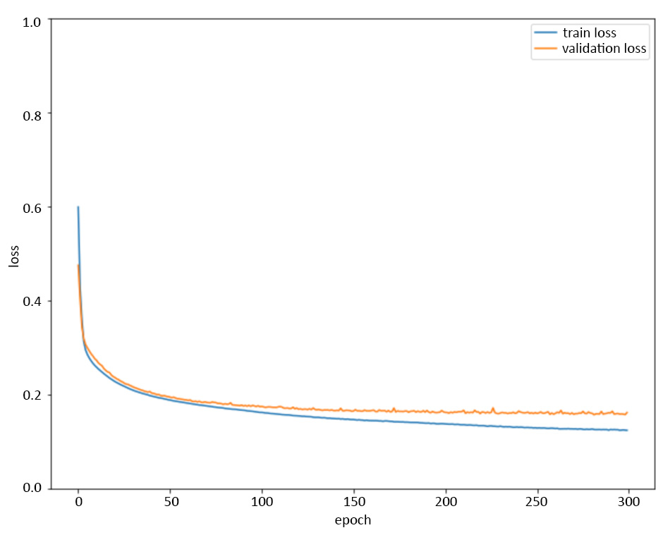
Figure 5.9: Plot of the training error and validation error while training the model without early stopping
As you can see from the preceding plot, training the model for 300 epochs results in a gap that grows between the training error and validation error, which is indicative of overfitting beginning to happen.
- Redefine the model by creating the model with the same number of layers and with the same number of units within each layer. This ensures the model is initialized in the same way. Add a callback es_callback = EarlyStopping(monitor='val_loss', mode='min') to the training process. Repeat step 4 to plot the training error and validation error:
#Define your model with early stopping on test error
from keras.callbacks import EarlyStopping
np.random.seed(seed)
random.set_seed(seed)
model_2 = Sequential()
model_2.add(Dense(16, activation='relu',
input_dim=X_train.shape[1]))
model_2.add(Dense(8, activation='relu'))
model_2.add(Dense(4, activation='relu'))
model_2.add(Dense(1, activation='sigmoid'))
"""
Choose the loss function to be binary cross entropy and the optimizer to be SGD for training the model
"""
model_2.compile(optimizer='sgd', loss='binary_crossentropy')
# define the early stopping callback
es_callback = EarlyStopping(monitor='val_loss',
mode='min')
# train the model
history=model_2.fit(X_train, y_train,
validation_data=(X_test, y_test),
epochs=300, batch_size=50,
callbacks=[es_callback], verbose=0,
shuffle=False)
- Now plot the loss values:
# plot training error and test error
matplotlib.rcParams['figure.figsize'] = (10.0, 8.0)
plt.plot(history.history['loss'])
plt.plot(history.history['val_loss'])
plt.ylim(0,1)
plt.ylabel('loss')
plt.xlabel('epoch')
plt.legend(['train loss', 'validation loss'],
loc='upper right')
Here's the expected output:

Figure 5.10: Plot of training error and validation error while training the model with early stopping (patience=0)
By adding the early stopping callback with patience=0 to the model, the training process automatically stops after about 39 epochs.
- Repeat step 5 while adding patience=10 to your early stopping callback. Repeat step 3 to plot the training error and validation error:
"""
Define your model with early stopping on test error with patience=10
"""
from keras.callbacks import EarlyStopping
np.random.seed(seed)
random.set_seed(seed)
model_3 = Sequential()
model_3.add(Dense(16, activation='relu',
input_dim=X_train.shape[1]))
model_3.add(Dense(8, activation='relu'))
model_3.add(Dense(4, activation='relu'))
model_3.add(Dense(1, activation='sigmoid'))
"""
Choose the loss function to be binary cross entropy and the optimizer to be SGD for training the model
"""
model_3.compile(optimizer='sgd', loss='binary_crossentropy')
# define the early stopping callback
es_callback = EarlyStopping(monitor='val_loss',
mode='min', patience=10)
# train the model
history=model_3.fit(X_train, y_train,
validation_data=(X_test, y_test),
epochs=300, batch_size=50,
callbacks=[es_callback], verbose=0,
shuffle=False)
- Then plot the loss again:
# plot training error and test error
matplotlib.rcParams['figure.figsize'] = (10.0, 8.0)
plt.plot(history.history['loss'])
plt.plot(history.history['val_loss'])
plt.ylim(0,1)
plt.ylabel('loss')
plt.xlabel('epoch')
plt.legend(['train loss', 'validation loss'],
loc='upper right')
Here's the expected output:
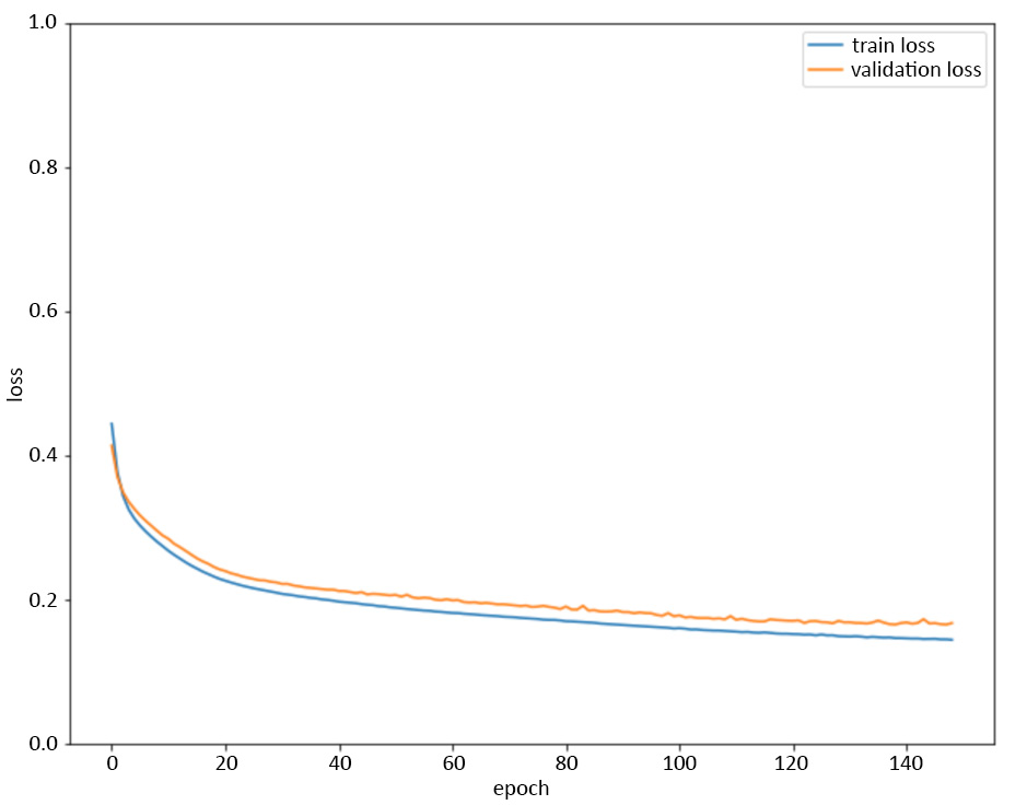
Figure 5.11: Plot of training error and validation error while training the model with early stopping (patience=10)
By adding the early stopping callback with patience=10 to the model, the training process automatically stops after about 150 epochs.
In this exercise, you learned how to stop the model to prevent your Keras model from overfitting the training data. To do this, you utilized the EarlyStopping callback and trained the model with it. We used this callback to stop the model any time the validation loss increased and added a patience parameter, which waits for a given number of epochs before stopping. We practiced using this callback on a problem involving the Traffic Volume dataset to train our Keras model.
Note
To access the source code for this specific section, please refer to https://packt.live/3iuM4eL.
You can also run this example online at https://packt.live/38AbweB.
In the next section, we will discuss other regularization methods that can be applied to prevent overfitting.
Data Augmentation
Data augmentation is a regularization technique that tries to address overfitting by training the model on more training examples in an inexpensive way. In data augmentation, the available data is transformed in different ways and fed to the model as new training data. This type of regularization has been shown to be effective, especially for some specific applications, such as object detection/recognition in computer vision and speech processing.
For example, in computer vision applications, you can simply double or triple the size of your training dataset by adding mirrored versions and rotated versions of each image to the dataset. The new training examples that are generated by these transformations are obviously not as good as the original training examples. However, they are shown to improve the model in terms of overfitting.
One challenging aspect of performing data augmentation is choosing the right transformations to be performed on data. Transformations need to be selected carefully, depending on the type of dataset and the application.
Adding Noise
The underlying idea behind regularizing a model by adding noise to the data is the same as that for data augmentation regularization. Training a deep neural network on a small dataset increases the chance of the network memorizing single data examples as opposed to capturing the relations between inputs and outputs.
This will result in poor performance on new data later, which is indicative of the model overfitting the training data. In contrast, training a model on a large dataset increases the chance of the model capturing the true underlying process instead of memorizing single data points, and therefore reduces the chances of overfitting.
One way to expand the training data and reduce overfitting is to generate new data examples by injecting noise into the available data. This type of regularization has been shown to reduce overfitting to an extent that is comparable to weight regularization techniques.
By adding different versions of a single example to the training data (each created by adding a small amount of noise to the original example), we can ensure that the model will not fit the noise in the data. Additionally, increasing the size of the training dataset by including these modified examples provides the model with a better representation of the underlying data generation process and increases the chance of the model learning the true process.
In deep learning applications, you can improve model performance by adding noise to the weights or activations of the hidden layers, or gradients of the network, or even to the output layer, as well as by adding noise to the training examples (input layer). Deciding where to add noise in a deep neural network is another challenge that needs to be addressed by trying different networks and observing the results.
In Keras, you can easily define noise as a layer and add it to your model. For example, to add Gaussian noise with a standard deviation of 0.1 (the mean is equal to 0) to your model, you can write this:
from keras.layers import GaussianNoise
model.add(GaussianNoise(0.1))
The following code will add Gaussian noise to the outputs/activations of the first hidden layer of the model:
model = Sequential()
model.add(Dense(4, input_dim=30, activation='relu'))
model.add(GaussianNoise(0.01))
model.add(Dense(4, activation='relu'))
model.add(Dense(4, activation='relu'))
model.add(Dense(1, activation='sigmoid'))
In this section, you learned about three regularization methods: early stopping, data augmentation, and adding noise. In addition to their basic concepts and procedures, you also learned about how they reduce overfitting and were given some tips and recommendations on how to use them. In the next section, you will learn how to tune hyperparameters using functions provided by scikit-learn. By doing this, we can incorporate Keras models into a scikit-learn workflow.
Hyperparameter Tuning with scikit-learn
Hyperparameter tuning is a very important technique for improving the performance of deep learning models. In Chapter 4, Evaluating Your Model with Cross-Validation Using Keras Wrappers, you learned about using a Keras wrapper with scikit-learn, which allows for Keras models to be used in a scikit-learn workflow. As a result, different general machine learning and data analysis tools and methods that are available in scikit-learn can be applied to Keras deep learning models. Among those methods are scikit-learn hyperparameter optimizers.
In the previous chapter, you learned how to perform hyperparameter tuning by writing user-defined functions to loop over possible values for each hyperparameter. In this section, you will learn how to perform it in a much easier way by using the various hyperparameter optimization methods that are available in scikit-learn. You will also get to practice applying those methods by completing an activity involving a real-life dataset.
Grid Search with scikit-learn
So far, we have established that building deep neural networks involves making decisions about several hyperparameters. The list of hyperparameters includes the number of hidden layers, the number of units in each hidden layer, the activation function for each layer, the loss function for the network, the type of optimizer and its parameters, the type of regularizer and its parameters, the batch size, the number of epochs, and others. We also observed that different values of hyperparameters can affect the performance of a model significantly.
Therefore, finding the best values for hyperparameters is one of the most important and challenging parts of becoming a deep learning expert. Since there are no absolute rules for picking the hyperparameters that work for every dataset and every problem, deciding on the values of hyperparameters needs to be done through trial and error for each particular problem. This process of training and evaluating models with different hyperparameters and deciding about the final hyperparameters based on model performance is called hyperparameter tuning or hyperparameter optimization.
Having a range or a set of possible values for each hyperparameter that we are interested in tuning can create a grid such as the one shown in the following image. Therefore, hyperparameter tuning can be seen as a grid search problem; we would like to try every cell in the grid (every possible combination of hyperparameters) and find the one cell that results in the best performance for the model:

Figure 5.12: A hyperparameter grid created by some values for optimizer, batch_size, and epochs
Scikit-learn provides a parameter optimizer called GridSearchCV() to perform this exhaustive grid search. GridSearchCV() receives the model as the estimator argument and the dictionary containing all possible values for the hyperparameters as the param_grid argument. Then, it goes through every point in the grid, performs cross-validation on the model using the hyperparameter values at that point, and returns the best cross-validation score, along with the values of the hyperparameters that led to that score.
In the previous chapter, you learned that in order to use Keras models in scikit-learn, you need to define a function that returns a Keras model. For example, the following code block defines a Keras model that we would like to perform hyperparameter tuning on later:
from keras.models import Sequential
from keras.layers import Dense
def build_model():
model = Sequential(optimizer)
model.add(Dense(10, input_dim=X_train.shape[1],
activation='relu'))
model.add(Dense(10, activation='relu'))
model.add(Dense(1))
model.compile(loss='mean_squared_error',
optimizer= optimizer)
return model
The next step would be to define the grid of parameters. For example, say we would like to tune over optimizer=['rmsprop', 'adam', 'sgd', 'adagrad'], epochs = [100, 150], batch_size = [1, 5, 10]. To do so, we would write the following:
optimizer = ['rmsprop', 'adam', 'sgd', 'adagrad']
epochs = [100, 150]
batch_size = [1, 5, 10]
param_grid = dict(optimizer=optimizer, epochs=epochs,
batch_size= batch_size)
Now that the hyperparameter grid has been created, we can create the wrapper so that we can build the interface for the Keras model and use it as an estimator to perform the grid search:
from keras.wrappers.scikit_learn import KerasRegressor
model = KerasRegressor(build_fn=build_model,
verbose=0, shuffle=False)
from sklearn.model_selection import GridSearchCV
grid_search = GridSearchCV(estimator=model,
param_grid=param_grid, cv=10)
results = grid_search.fit(X, y)
The preceding code through goes through every cell in the grid exhaustively and performs 10-fold cross-validation using hyperparameter values in each cell (here, it performs 10-fold cross-validation 4*2*3=24 times). Then, it returns the cross-validation score for each of these 24 cells, along with the one that resulted in the best score.
Note
Performing k-fold cross-validation on many possible combinations of hyperparameters sure takes a long time. For this reason, you can parallelize the process by passing the n_jobs=-1 argument to GridSearchCV(), which results in using every processor available to perform the grid search. The default value for this argument is n_jobs=1, which means no parallelization.
Creating a hyperparameter grid is just one way to iterate through hyperparameters to find the optimal selection. Another way is to simply randomize the selection of hyperparameters, which we will learn about in the next topic.
Randomized Search with scikit-learn
As you may have realized, an exhaustive grid search may not be the best choice for tuning the hyperparameters of a deep learning model since it is not very efficient. There are many hyperparameters in deep learning, and especially if you would like to try a large range of values for each, an exhaustive grid search would simply take too long to complete. An alternative way to perform hyperparameter optimization is to perform random sampling on the grid and perform k-fold cross-validation on some randomly selected cells. Scikit-learn provides an optimizer called RandomizedSearchCV() to perform a random search for the purpose of hyperparameter optimization.
For example, we can change the code from the previous section from an exhaustive grid search to a random search like so:
from keras.wrappers.scikit_learn import KerasRegressor
model = KerasRegressor(build_fn=build_model, verbose=0)
from sklearn.model_selection import RandomizedSearchCV
grid_search = RandomizedSearchCV(estimator=model,
param_distributions=param_grid,
cv=10, n_iter=12)
results = grid_search.fit(X, y)
Notice that RandomizedSearchCV() requires the extra n_iter argument, which determines how many random cells must be selected. This determines how many times k-fold cross-validation will be performed. Therefore, by choosing a smaller number, fewer hyperparameter combinations will be considered and the method will take less time to complete. Also, please note that the param_grid argument is changed to param_distributions here. The param_distributions argument can take a dictionary with parameter names as keys, and either list of parameters or distributions as values for each key.
It could be argued that RandomizedSearchCV() is not as good as GridSearchCV() since it does not consider all the possible values and combinations of values for hyperparameters, which is reasonable. As a result, one smart way of performing hyperparameter tuning for deep learning models is to start with either RandomizedSearchCV() on many hyperparameters, or GridSearchCV() on fewer hyperparameters with larger gaps between them.
By beginning with a randomized search on many hyperparameters, we can determine which hyperparameters have the most influence on a model's performance. It can also help narrow down the range for important hyperparameters. Then, you can complete your hyperparameter tuning by performing GridSearchCV() on the smaller number of hyperparameters and the smaller ranges for each of them. This is called the coarse-to-fine approach to hyperparameter tuning.
Now, you are ready to practice implementing hyperparameter tuning using scikit-learn optimizers. In the next activity, you will try to improve your model for the diabetes dataset by tuning the hyperparameters.
Activity 5.03: Hyperparameter Tuning on the Avila Pattern Classifier
The Avila dataset has been extracted from 800 images of the Avila Bible, a giant 12th-century Latin copy of the Bible. The dataset consists of various features about the images of the text, such as intercolumnar distance and margins of the text. The dataset also contains a class label that indicates if the pattern of the image falls into the most frequently occurring category or not. In this activity, you will build a Keras model similar to those in the previous activities, but this time, you will add regularization methods to your model as well. Then, you will use scikit-learn optimizers to perform tuning on the model hyperparameters, including the hyperparameters of the regularizers. Here are the steps you need to complete in this activity:
- Load the dataset from the data subfolder of the Chapter05 folder from GitHub using X = pd.read_csv('../data/avila-tr_feats.csv') and y = pd.read_csv('../data/avila-tr_target.csv').
- Define a function that returns a Keras model with three hidden layers, the first of size 10, the second of size 6, and the third of size 4, all with L2 weight regularizations. Use these values as the hyperparameters for your model: activation='relu', loss='binary_crossentropy', optimizer='sgd', and metrics=['accuracy']. Also, make sure to pass the L2 lambda hyperparameter as an argument to your function so that we can tune it later.
- Create the wrapper for your Keras model and perform GridSearchCV() on it using cv=5. Then, add the following values in the parameter grid: lambda_parameter = [0.01, 0.5, 1], epochs = [50, 100], and batch_size = [20]. This might take some time to process. Once the parameter search is complete, print the accuracy and the hyperparameters of the best cross-validation score. You can also print every other cross-validation score, along with the hyperparameters that resulted in that score.
- Repeat the previous step, this time using GridSearchCV() on a narrower range with lambda_parameter = [0.001, 0.01, 0.05, 0.1], epochs = [400], and batch_size = [10]. It might take some time to process.
- Repeat the previous step, but remove the L2 regularizers from your Keras model and instead of adding dropout regularization with the rate parameter at each hidden layer. Perform GridSearchCV() on the model using the following values in the parameter grid and print the results: rate = [0, 0.2, 0.4], epochs = [350, 400], and batch_size = [10].
- Repeat the previous step using rate = [0.0, 0.05, 0.1] and epochs=[400].
After implementing these steps, you should see the following expected output:
Best cross-validation score= 0.7862895488739013
Parameters for Best cross-validation score= {'batch_size': 20, 'epochs': 100, 'rate': 0.0}
Accuracy 0.786290 (std 0.013557) for params {'batch_size': 20, 'epochs': 100, 'rate': 0.0}
Accuracy 0.786098 (std 0.005184) for params {'batch_size': 20, 'epochs': 100, 'rate': 0.05}
Accuracy 0.772004 (std 0.013733) for params {'batch_size': 20, 'epochs': 100, 'rate': 0.1}
Note
The solution for this activity can be found on page 422.
In this activity, we learned how to implement hyperparameter tuning on a Keras model with regularizers to perform classification using a real-life dataset. We learned how to use scikit-learn optimizers to perform tuning on model hyperparameters, including the hyperparameters of the regularizers. In this section, we implemented hyperparameter tuning by creating a grid of hyperparameters and iterating through them. This allows us to find the optimal set of hyperparameters using a scikit-learn workflow.
Summary
In this chapter, you learned about two very important groups of techniques for improving the accuracy of your deep learning models: regularization and hyperparameter tuning. You learned how regularization helps address the overfitting problem by means of several different methods, including L1 and L2 norm regularization and dropout regularization—the more commonly used regularization techniques. You discovered the importance of hyperparameter tuning for machine learning models and the challenge of hyperparameter tuning for deep learning models in particular. You even practiced using scikit-learn optimizers to perform hyperparameter tuning on Keras models.
In the next chapter, you will explore the limitations of accuracy metrics when evaluating model performance, as well as other metrics (such as precision, sensitivity, specificity, and AUC-ROC score), including how to use them in order to gauge the quality of your model's performance better.