Overview
This chapter covers computer vision and how this is accomplished with neural networks. You will learn to build image processing applications and classify models with convolutional neural networks. You will also study the architecture of convolutional neural networks and how to utilize techniques such as max pooling and flattening, feature mapping, and feature detection. By the end of this chapter, you will be able to not only build your own image classifiers but also evaluate them effectively for your own applications.
Introduction
In the previous chapter, we explored model evaluation in detail. We covered accuracy and why it may be misleading for some datasets, especially for classification tasks with highly imbalanced classes. Datasets with imbalanced classes such as the prediction of hurricanes in the Pacific Ocean or the prediction of whether someone will default on their credit card loan have positive instances that are relatively rare compared to negative instances, so accuracy scores are misleading since the null accuracy is so high.
To combat class imbalance, we learned about techniques that we can use to appropriately evaluate our model, including calculating model evaluation metrics such as the sensitivity, specificity, false positive rate, and AUC score, and plotting the ROC curve. In this chapter, we will learn how to classify another type of dataset—namely, images. Image classification is extremely useful and there are many real-world applications of it, as we will discover.
Computer vision is one of the most important concepts in machine learning and artificial intelligence. With the wide use of smartphones for capturing, sharing, and uploading images every day, the amount of data that's generated through images is increasing exponentially. So, the need for experts who are specialized in the field of computer vision is at an all-time high. Industries such as the health care industry are on the verge of a revolution due to the progress that's been made in the field of medical imaging.
This chapter will introduce you to computer vision and the various industries in which computer vision is used. You will also learn about Convolutional Neural Networks (CNNs), which are the most widely used neural networks for image processing. Like neural networks, CNNs are also made up of neurons that receive inputs that are processed using weighted sums and activation functions. However, unlike ANNs, which use vectors as inputs, CNN uses images as its input. In this chapter, we will be studying CNNs in greater detail, along with the associated concepts of max pooling, flattening, feature maps, and feature selection. We will use Keras as a tool to run image processing algorithms on real-life images.
Computer Vision
To understand computer vision, let's discuss human vision. Human vision is the ability of the human eye and brain to see and recognize objects. Computer vision is the process of giving a machine a similar, if not better, understanding of seeing and identifying objects in the real world.
It is fairly simple for the human eye to precisely identify whether an animal is a tiger or a lion, but it takes a lot of training for a computer system to understand such objects distinctly. Computer vision can also be defined as building mathematical models that can mimic the function of a human eye and brain. Basically, it is about training computers to understand and process images and videos.
Computer vision is an integral part of many cutting-edge areas of robotics: health care and medical (X-rays, MRI scans, CT scans, and so on), drones, self-driving cars, sports and recreation, and so on. Almost all businesses need computer vision to run successfully.
Imagine a large amount of data that's generated by CCTV footage across the world, the number of pictures our smartphones capture each day, the number of videos that are shared on internet sites such as YouTube on a daily basis, and the pictures we share on popular social networking sites such as Facebook and Instagram. All of this generates huge volumes of image data. To process and analyze this data and make computers more intelligent in terms of processing, this data requires high-level experts who specialize in computer vision. Computer vision is a highly lucrative field in machine learning. The following sections will describe how computer vision is achieved with neural networks—and particularly convolutional neural networks—that perform well for computer vision tasks.
Convolutional Neural Networks
When we talk about computer vision, we talk about CNNs in the same breath. CNN is a class of deep neural network that is mostly used in the field of computer vision and imaging. CNNs are used to identify images, cluster them by their similarity, and implement object recognition within scenes. CNN has different layers— namely, the input layer, the output layer, and multiple hidden layers. These hidden layers of a CNN consist of fully connected layers, convolutional layers, a ReLU layer as an activation function, normalization layers, and pooling layers. On a very simple level, CNNs help us identify images and label them appropriately; for example, a tiger image will be identified as a tiger:

Figure 7.1: A generalized CNN
The following is an example of a CNN classifying a tiger:

Figure 7.2: A CNN classifying an image of a tiger into the class "Tiger"
The Architecture of a CNN
The main components of CNN architecture are as follows:
- Input image
- Convolutional layer
- Pooling layer
- Flattening
Input Image
An input image forms the first component of a CNN architecture. An image can be of any type: a human, an animal, scenery, a medical X-ray image, and so on. Each image is converted into a mathematical matrix of zeros and ones. The following figure explains how a computer views an image of the letter T.
All the blocks that have a value of one represent the data, while the zeros represent blank space:
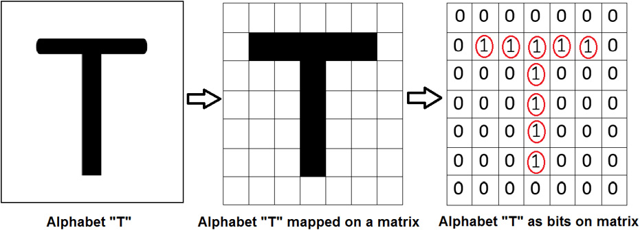
Figure 7.3: Matrix for the letter 'T'
Convolution Layer
The convolution layer is the place where image processing starts. A convolution layer consists of two parts:
- Feature detector or filter
- Feature map
Feature detector or a filter: This is a matrix or pattern that you put on an image to transform it into a feature map:

Figure 7.4: Feature detector
As we can see, this feature detector is put (superimposed) on the original image and the computation is done on the corresponding elements. The computation is done by multiplying the corresponding elements, as shown in the following figure. This process is repeated for all the cells. This results in a new processed image— (0x0+0x0+0x1) + (0x1+1x0+0x0) + (0x0+0x1+0x1) = 0:

Figure 7.5: Feature detector masked in an image
Feature Map: This is the reduced image that is produced by the convolution of an image and feature detector. We have to put the feature detector on all the possible locations of the original image and derive a smaller image from it; that derived image is the feature map of the input image:

Figure 7.6: Feature map
Note
Here, the feature detector is the filter and the feature map is the reduced image. Some information is lost while reducing the image.
In an actual CNN, a number of feature detectors are used to produce a number of feature maps, as shown in the following figure:
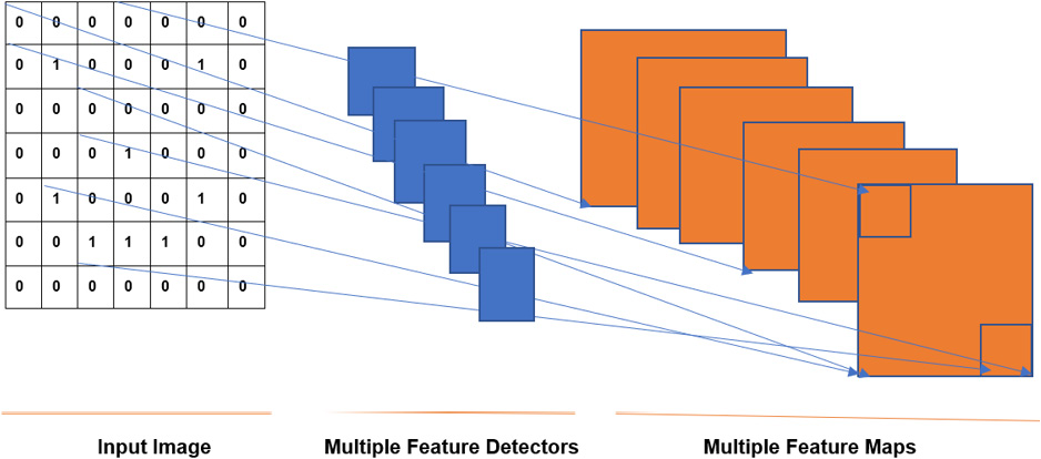
Figure 7.7: Multiple feature detectors and maps
The Pooling Layer
The pooling layer helps us ignore the less important data in the image and reduces the image further, all while preserving its important features. Consider the following three images, which contain four cats in total:
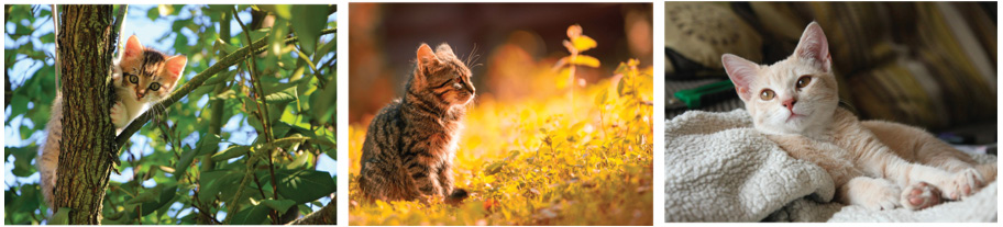
Figure 7.8: Example of cat images
To identify whether an image has a cat in it or not, the neural network analyzes the picture. It may look at ear shape, eye shape, and so on. At the same time, the image consists of lots of features that are not related to cats. The tree and leaves in the first two images are useless in the identification of the cat. The pooling mechanism helps the algorithm understand which parts of the image are relevant and which parts are irrelevant.
The feature map derived from the convolution layer is passed through a pooling layer to further reduce the image, all while preserving the most relevant part of the image. The pooling layer consists of functions such as max pooling, min pooling, and average pooling. What this means is that we select a matrix size, say 2x2, and we scan the feature map and select the maximum number from the 2x2 matrix that fits in that block. The following image gives us a clear idea of how max pooling works. Refer to the colors; the max number in each of the colored boxes from the feature map is selected in the pooled feature map:
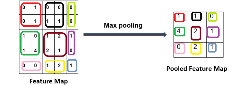
Figure 7.9: Pooling
Consider the case of the box that has number 4 in it. Let's assume that number 4 represents the ears of a cat, while the blank space around the ears is 0 and 1. So, we ignore the 0 and 1 of that block and only select 4. The following is some example code that we would use to add a pooling layer; here, Maxpool2D is used for max pooling, which helps identify the most important features:
classifier.add(MaxPool2D(2,2))
Flattening
Flattening is part of a CNN where the image is made ready to use as an input to an ANN. As the name suggests, the pooled image is flattened and converted into a single column. Each row is made into a column and stacked one over another. Here, we have converted a 3x3 matrix into a 1xn matrix, where n, in our case, is 9:

Figure 7.10: Flattening
In real-time, we have a number of pooled feature maps, and we flatten them into a single column. This single column is used as input for an ANN. The following figure shows a number of pooled layers flattened into a single column:

Figure 7.11: Pooling and flattening
The following is some example code that we would use to add a flattening layer; here Flatten is used for flattening the CNN:
classifier.add(Flatten())
Now, let's look at the overall structure of a CNN:

Figure 7.12: CNN architecture
The following is some example code that we would use to add the first layer to a CNN:
classifier.add(Conv2D(32,3,3,input_shape=(64,64,3),activation='relu'))
32,3,3 refers to the fact that there are 32 feature detectors of size 3x3. As a good practice, always start with 32; you can add 64 or 128 later.
Input_shape: Since all the images are of different shapes and sizes, this input_image converts all the images into a uniform shape and size. (64,64) is the dimension of the converted image. It can be set to 128 or 256, but if you are working on a CPU on a laptop, it is advisable to use 64x64. The last argument, 3, is used because the image is a colored image (coded in red, blue, and green, or RGB). If the image is black and white, the argument can be set to one. The activation function that's being used is ReLU.
Note
We are using Keras with TensorFlow as the backend in this book. If the backend is Theano, then input_image will be coded as (3,64,64).
The last step is to fit the data that's been created. Here is the code that we use to do so:
classifier.fit_generator(training_set,steps_per_epoch = 5000,
epochs = 25,validation_data = test_set,
validation_steps = 1000)
Note
steps_per_epoch is the number of training images. validation_steps is the number of test images.
Image Augmentation
The word augmentation means the action or process of making or becoming greater in size or amount. Image or data augmentation works in a similar manner. Image/data augmentation creates many batches of our images. Then, it applies random transformations to random images inside the batches. Data transformation can be rotating images, shifting them, flipping them, and so on. By applying this transformation, we get more diverse images inside the batches, and we also have much more data than we had originally.
A cylinder can be rotated from different angles and seen differently. In the following figure, a single cylinder can be seen from five different angles. So, we have effectively created five different images from a single image:
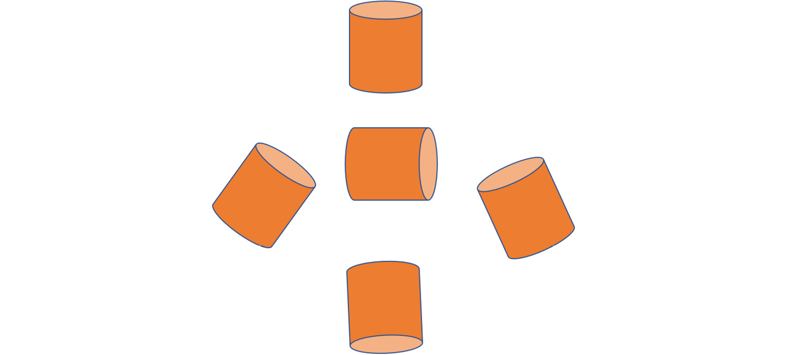
Figure 7.13: Image augmentation of a cylinder
The following is some example code that we would use for image augmentation; here, the ImageDataGenerator class is used for processing. shear_range, zoom_range, and horizontal_flip are all used for transforming the images:
from keras.preprocessing.image import ImageDataGenerator
train_datagen = ImageDataGenerator(rescale = 1./255.0,
shear_range = 0.3,
zoom_range = 0.3,
horizontal_flip = False)
test_datagen = ImageDataGenerator(rescale = 1./255.0)
Advantages of Image Augmentation
Image augmentation is an important part of processing images:
- Reduces overfitting: It helps reduce overfitting by creating multiple versions of the same image, rotated by a given amount.
- Increases the number of images: A single image acts as multiple images. So, essentially, the dataset has fewer images, but each image can be converted into multiple images with image augmentation. Image augmentation will increase the number of images and each image will be treated differently by the algorithm.
- Easy to predict new images: Imagine that a single image of a football is looked at from different angles and each angle is considered a distinct image. This will mean that the algorithm will be more accurate at predicting new images:
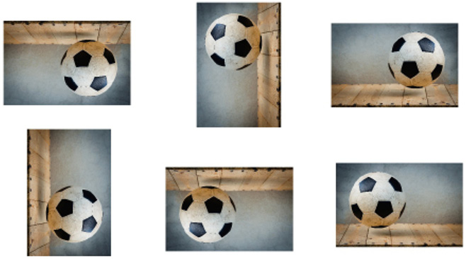
Figure 7.14: Image augmentation of an image of a football
Now that we have learned about the concepts and theory behind computer vision with CNNs, let's work on some practical examples.
First, we will start with an exercise in which we'll build a simple CNN. In the following exercises and activities, we will tweak our CNN using permutation and combining the following:
- Adding more CNN layers
- Adding more ANN layers
- Changing the optimizer function
- Changing the activation function
Let's begin by creating our first CNN so that we can classify images of cars and flowers into their respective classes.
Exercise 7.01: Building a CNN and Identifying Images of Cars and Flowers
For this exercise, we have images of cars and flowers, which have been divided into training and testing sets, and we have to build a CNN that identifies whether an image is a car or a flower.
Note
All the exercises and activities in this chapter will be developed in Jupyter notebooks. Please download this book's GitHub repository, along with all the prepared templates, from https://packt.live/39tID2C.
Before you begin, ensure that you have downloaded the image datasets from this book's GitHub repository to your own working directory. You will need a training_set folder to train your model and a test_set folder to test your model. Each of these folders will contain a cars folder, containing car images, and a flowers folder, containing flower images.
The steps for completing this exercise are as follows:
- Import the numpy library and the necessary Keras libraries and classes:
# Import the Libraries
from keras.models import Sequential
from keras.layers import Conv2D, MaxPool2D, Flatten, Dense
import numpy as np
from tensorflow import random
- Now, set a seed and initiate the model with the Sequential class:
# Initiate the classifier
seed = 1
np.random.seed(seed)
random.set_seed(seed)
classifier = Sequential()
- Add the first layer of the CNN, set the input shape to (64, 64, 3), the dimension of each image, and set the activation function as a ReLU:
classifier.add(Conv2D(32,3,3, input_shape=(64,64,3),
activation='relu'))
32,3,3 shows that there are 32 feature detectors of 3x3 size.
- Now, add the pooling layer with the image size as 2x2:
classifier.add(MaxPool2D(2,2))
- Flatten the output of the pooling layer by adding a flattening layer to the CNN model:
classifier.add(Flatten())
- Add the first Dense layer of the ANN. Here, 128 is the output of the number of nodes. As a good practice, 128 is good to get started. activation is relu. As a good practice, the power of two is preferred:
classifier.add(Dense(128, activation='relu'))
- Add the output layer of the ANN. This is a binary classification problem, so the size is 1 and the activation is sigmoid:
classifier.add(Dense(1, activation='sigmoid'))
- Compile the network with an adam optimizer and compute the accuracy during the training process:
#Compile the network
classifier.compile(optimizer='adam', loss='binary_crossentropy',
metrics=['accuracy'])
- Create training and test data generators. Rescale the training and test images by 1/255 so that all the values are between 0 and 1. Set these parameters for the training data generators only – shear_range=0.2, zoom_range=0.2, and horizontal_flip=True:
from keras.preprocessing.image import ImageDataGenerator
train_datagen = ImageDataGenerator(rescale = 1./255,
shear_range = 0.2,
zoom_range = 0.2,
horizontal_flip = True)
test_datagen = ImageDataGenerator(rescale = 1./255)
- Create a training set from the training set folder. '../dataset/training_set' is the folder where our data has been placed. Our CNN model has an image size of 64x64, so the same size should be passed here too. batch_size is the number of images in a single batch, which is 32. Class_mode is set to binary since we are working on binary classifiers:
training_set = train_datagen.flow_from_directory(
'../dataset/training_set',
target_size = (64, 64),
batch_size = 32,
class_mode = 'binary')
- Repeat step 10 for the test set while setting the folder to the location of the test images, that is, '../dataset/test_set':
test_set = test_datagen.flow_from_directory(
'../dataset/test_set',
target_size = (64, 64),
batch_size = 32,
class_mode = 'binary')
- Finally, fit the data. Set the steps_per_epoch to 10000 and the validation_steps to 2500. The following step might take some time to execute:
classifier.fit_generator(training_set,steps_per_epoch = 10000,
epochs = 2,validation_data = test_set,
validation_steps = 2500,shuffle=False)
The preceding code produces the following output:
Epoch 1/2
10000/10000 [==============================] - 1994s 199ms/step - loss: 0.2474 - accuracy: 0.8957 - val_loss: 1.1562 - val_accuracy: 0.8400
Epoch 2/2
10000/10000 [==============================] - 1695s 169ms/step - loss: 0.0867 - accuracy: 0.9689 - val_loss: 1.4379 - val_accuracy: 0.8422
The accuracy on the validation set is 84.22%.
Note
To get more accurate results, try increasing the number of epochs to about 25. This will increase the time that it takes to process the data, and the total time is dependent on the configuration of your machine.
To access the source code for this specific section, please refer to https://packt.live/38njqHU.
You can also run this example online at https://packt.live/3iqFpSN.
That completes this exercise on processing images and identifying the contents of the images. An important thing to remember here is that this is a robust code for any binary classification problem in computer vision. This means that the code remains the same, even if the image data changes. We will test our knowledge of this by modifying some of the parameters of our model in the next activity and evaluating the model's performance.
Activity 7.01: Amending Our Model with Multiple Layers and the Use of softmax
Since we have run a CNN model successfully, the next logical step is to try and improve the performance of our algorithm. There are many ways to improve its performance, and one of the most straightforward ways is by adding multiple ANN layers to the model, which we will learn about in this activity. We will also change the activation from sigmoid to softmax. By doing this, we can compare the result with that of the previous exercise. Follow these steps to complete this activity:
- To build a CNN import library, set a seed and create a Sequential class and import Conv2D, MaxPool2D, Flatten, and Dense. Conv2D is used to build the convolution layer. Since our pictures are in 2D, we have used 2D here. Similarly, Maxpool2D is used for max pooling, Flatten is used for flattening the CNN, and Dense is used to add a fully connected CNN to an ANN.
- Start building a CNN architecture using the preceding libraries. After adding the first layer, add two additional layers to your CNN.
- Add a pooling and flattening layer to it, which will serve as the input for the ANN.
- Build a fully connected ANN whose inputs will be the output of the CNN. After adding the first layer of your ANN, add three additional layers. For the output layer of your ANN, use the softmax activation function. Compile the model.
- Perform image augmentation to process and transform the data. The ImageDataGenerator class is used for processing. shear_range, zoom_range, and horizontal_flip are all used for the transformation of images.
- Create the training and test set data.
- Lastly, fit the data that's been created.
After implementing these steps, you should get the following expected output:
Epoch 1/2
10000/10000 [==============================] - 2452s 245ms/step - loss: 8.1783 - accuracy: 0.4667 - val_loss: 11.4999 - val_accuracy: 0.4695
Epoch 2/2
10000/10000 [==============================] - 2496s 250ms/step - loss: 8.1726 - accuracy: 0.4671 - val_loss: 10.5416 - val_accuracy: 0.4691
Note
The solution for this activity can be found on page 439.
In this activity, we have modified our CNN model to try and improve the accuracy of our image classifier. We have added additional convolutional layers and additional ANN fully connected layers and changed the activation function in the output layer. By doing so our accuracy has decreased. In the next exercise, we will change the activation function back to a sigmoid. We will evaluate the performance by observing the accuracy evaluated on the validation dataset.
Exercise 7.02: Amending Our Model by Reverting to the Sigmoid Activation Function
In this exercise, we will rebuild our model but revert the activation function from softmax back to sigmoid. By doing this, we can compare the accuracy with our previous model's. Follow these steps to complete this exercise:
- Import the numpy library and the necessary Keras libraries and classes:
# Import the Libraries
from keras.models import Sequential
from keras.layers import Conv2D, MaxPool2D, Flatten, Dense
import numpy as np
from tensorflow import random
- Now, set the seed and initiate the model with the Sequential class:
# Initiate the classifier
seed = 43
np.random.seed(seed)
random.set_seed(seed)
classifier = Sequential()
- Add the first layer of the CNN, set the input shape to (64, 64, 3), the dimension of each image, and set the activation function as a ReLU. Then, add 32 feature detectors of size (3, 3). Add two additional convolutional layers with 32 feature detectors of size (3, 3), also with ReLU activation functions:
classifier.add(Conv2D(32,3,3,input_shape=(64,64,3),
activation='relu'))
classifier.add(Conv2D(32, (3, 3), activation = 'relu'))
classifier.add(Conv2D(32, (3, 3), activation = 'relu'))
- Now, add the pooling layer with the image size as 2x2:
classifier.add(MaxPool2D(2,2))
- Add one more Conv2D with the same parameters as in step 3 and a pooling layer to supplement it with the same parameters that we used in step 4:
classifier.add(Conv2D(32, (3, 3), activation = 'relu'))
classifier.add(MaxPool2D(pool_size = (2, 2)))
- Flatten the output of the pooling layer by adding a flattening layer to the CNN model:
classifier.add(Flatten())
- Add the first Dense layer of the ANN. Here, 128 is the output of the number of nodes. As a good practice, 128 is good to get started. activation is relu. As a good practice, the power of two is preferred. Add three additional layers with the same parameters:
classifier.add(Dense(128,activation='relu'))
classifier.add(Dense(128,activation='relu'))
classifier.add(Dense(128,activation='relu'))
classifier.add(Dense(128,activation='relu'))
- Add the output layer of the ANN. This is a binary classification problem, so the output is 1 and the activation is sigmoid:
classifier.add(Dense(1,activation='sigmoid'))
- Compile the network with an Adam optimizer and compute the accuracy during the training process:
classifier.compile(optimizer='adam', loss='binary_crossentropy',
metrics=['accuracy'])
- Create training and test data generators. Rescale the training and test images by 1/255 so that all the values are between 0 and 1. Set these parameters for the training data generators only – shear_range=0.2, zoom_range=0.2, and horizontal_flip=True:
from keras.preprocessing.image import ImageDataGenerator
train_datagen = ImageDataGenerator(rescale = 1./255,
shear_range = 0.2,
zoom_range = 0.2,
horizontal_flip = True)
test_datagen = ImageDataGenerator(rescale = 1./255)
- Create a training set from the training set folder. ../dataset/training_set is the folder where our data is placed. Our CNN model has an image size of 64x64, so the same size should be passed here too. batch_size is the number of images in a single batch, which is 32. class_mode is binary since we are working on binary classifiers:
training_set =
train_datagen.flow_from_directory('../dataset/training_set',
target_size = (64, 64),
batch_size = 32,
class_mode = 'binary')
- Repeat step 11 for the test set by setting the folder to the location of the test images, that is, '../dataset/test_set':
test_set =
test_datagen.flow_from_directory('../dataset/test_set',
target_size = (64, 64),
batch_size = 32,
class_mode = 'binary')
- Finally, fit the data. Set the steps_per_epoch to 10000 and the validation_steps to 2500. The following step might take some time to execute:
classifier.fit_generator(training_set,steps_per_epoch = 10000,
epochs = 2,validation_data = test_set,
validation_steps = 2500,shuffle=False)
The preceding code produces the following output:
Epoch 1/2
10000/10000 [==============================] - 2241s 224ms/step - loss: 0.2339 - accuracy: 0.9005 - val_loss: 0.8059 - val_accuracy: 0.8737
Epoch 2/2
10000/10000 [==============================] - 2394s 239ms/step - loss: 0.0810 - accuracy: 0.9699 - val_loss: 0.6783 - val_accuracy: 0.8675
The accuracy of the model is 86.75%, which is clearly greater than the accuracy of the model we built in the previous exercise. This shows the importance of activation functions. Just changing the output activation function from softmax to sigmoid increased the accuracy from 46.91% to 86.75%.
Note
To access the source code for this specific section, please refer to https://packt.live/2ZD9nKM.
You can also run this example online at https://packt.live/3dPZiiQ.
In the next exercise, we will experiment with a different optimizer and observe how that affects the model's performance.
Note
In a binary classification problem (in our case, cars versus flowers), it is always better to use sigmoid as the activation function for the output.
Exercise 7.03: Changing the Optimizer from Adam to SGD
In this exercise, we will amend the model again by changing the optimizer to SGD. By doing this, we can compare the accuracy with our previous models. Follow these steps to complete this exercise:
- Import the numpy library and the necessary Keras libraries and classes:
# Import the Libraries
from keras.models import Sequential
from keras.layers import Conv2D, MaxPool2D, Flatten, Dense
import numpy as np
from tensorflow import random
- Now, initiate the model with the Sequential class:
# Initiate the classifier
seed = 42
np.random.seed(seed)
random.set_seed(seed)
classifier = Sequential()
- Add the first layer of the CNN, set the input shape to (64, 64, 3), the dimension of each image, and set the activation function as ReLU. Then, add 32 feature detectors of size (3, 3). Add two additional convolutional layers with the same number of feature detectors with the same size:
classifier.add(Conv2D(32,(3,3),input_shape=(64,64,3),
activation='relu'))
classifier.add(Conv2D(32,(3,3),activation='relu'))
classifier.add(Conv2D(32,(3,3),activation='relu'))
- Now, add the pooling layer with the image size as 2x2:
classifier.add(MaxPool2D(pool_size=(2, 2)))
- Add one more Conv2D with the same parameters as in step 3 and a pooling layer to supplement it with the same parameters that we used in step 4:
classifier.add(Conv2D(32, (3, 3), input_shape = (64, 64, 3),
activation = 'relu'))
classifier.add(MaxPool2D(pool_size=(2, 2)))
- Add a Flatten layer to complete the CNN architecture:
classifier.add(Flatten())
- Add the first Dense layer of the ANN of size 128. Add three more dense layers to the network with the same parameters:
classifier.add(Dense(128,activation='relu'))
classifier.add(Dense(128,activation='relu'))
classifier.add(Dense(128,activation='relu'))
classifier.add(Dense(128,activation='relu'))
- Add the output layer of the ANN. This is a binary classification problem, so the output is 1 and the activation is sigmoid:
classifier.add(Dense(1,activation='sigmoid'))
- Compile the network with an SGD optimizer and compute the accuracy during the training process:
classifier.compile(optimizer='SGD', loss='binary_crossentropy',
metrics=['accuracy'])
- Create training and test data generators. Rescale the training and test images by 1/255 so that all the values are between 0 and 1. Set these parameters for the training data generators only – shear_range=0.2, zoom_range=0.2, and horizontal_flip=True:
from keras.preprocessing.image import ImageDataGenerator
train_datagen = ImageDataGenerator(rescale = 1./255,
shear_range = 0.2,
zoom_range = 0.2,
horizontal_flip = True)
test_datagen = ImageDataGenerator(rescale = 1./255)
- Create a training set from the training set folder. ../dataset/training_set is the folder where our data is placed. Our CNN model has an image size of 64x64, so the same size should be passed here too. batch_size is the number of images in a single batch, which is 32. class_mode is binary since we are creating a binary classifier:
training_set =
train_datagen.flow_from_directory('../dataset/training_set',
target_size = (64, 64),
batch_size = 32,
class_mode = 'binary')
- Repeat step 11 for the test set by setting the folder to the location of the test images, that is, '../dataset/test_set':
test_set =
test_datagen.flow_from_directory('../dataset/test_set',
target_size = (64, 64),
batch_size = 32,
class_mode = 'binary')
- Finally, fit the data. Set the steps_per_epoch to 10000 and the validation_steps to 2500. The following step might take some time to execute:
classifier.fit_generator(training_set,steps_per_epoch = 10000,
epochs = 2,validation_data = test_set,
validation_steps = 2500,shuffle=False)
The preceding code produces the following output:
Epoch 1/2
10000/10000 [==============================] - 4376s 438ms/step - loss: 0.3920 - accuracy: 0.8201 - val_loss: 0.3937 - val_accuracy: 0.8531
Epoch 2/2
10000/10000 [==============================] - 5146s 515ms/step - loss: 0.2395 - accuracy: 0.8995 - val_loss: 0.4694 - val_accuracy: 0.8454
The accuracy is 84.54% since we have used multiple ANNs and SGD as the optimizer.
Note
To access the source code for this specific section, please refer to https://packt.live/31Hu9vm.
You can also run this example online at https://packt.live/3gqE9x8.
So far, we have worked with a number of different permutations and combinations of our model. It seems like the best accuracy for this dataset can be obtained by doing the following:
- Adding multiple CNN layers.
- Adding multiple ANN layers.
- Having the activation as sigmoid.
- Having the optimizer as adam.
- Increasing the epoch size to about 25 (this takes a lot of computational time – make sure you have a GPU to do this). This will increase the accuracy of your predictions.
Finally, we will go ahead and predict a new unknown image, pass it to the algorithm, and validate whether the image is classified correctly. In the next exercise, we will demonstrate how to use the model to classify new images.
Exercise 7.04: Classifying a New Image
In this exercise, we will try to classify a new image. The image hasn't been exposed to the algorithm, so we will use this exercise to test our algorithm. You can run any of the algorithms in this chapter (although the one that gets the highest accuracy is preferred) and then use the model to classify the image.
Note
The image that's being used in this exercise can be found in this book's GitHub repository at https://packt.live/39tID2C.
Before we begin, ensure that you have downloaded test_image_1 from this book's GitHub repository to your own working directory. This exercise follows on from the previous exercises, so ensure that you have one of the algorithms from this chapter ready to run in your workspace.
The steps for completing this exercise are as follows:
- Load the image. 'test_image_1.jpg' is the path of the test image. Please change the path to where you have saved the dataset in your system. Look at the image to verify what it is:
from keras.preprocessing import image
new_image = image.load_img('../test_image_1.jpg',
target_size = (64, 64))
new_image
- Print the class labels located in the class_indices attribute of the training set:
training_set.class_indices
- Process the image:
new_image = image.img_to_array(new_image)
new_image = np.expand_dims(new_image, axis = 0)
- Predict the new image:
result = classifier.predict(new_image)
- The prediction method will output the image as 1 or 0. To map 1 and 0 to flower or car, use the class_indices method with an if…else statement, as follows:
if result[0][0] == 1:
prediction = 'It is a flower'
else:
prediction = 'It is a car'
print(prediction)
The preceding code produces the following output:
It is a car
test_image_1 is the image of a car (you can see this by viewing the image for yourself) and was correctly predicted to be a car by the model.
In this exercise, we trained our model and then gave the model an image of a car. By doing this, we found out that the algorithm is classifying the image correctly. You can train the model on any type of an image by using the same process. For example, if you train the model with scans of lung infections and healthy lungs, then the model will be able to classify whether a new scan represents an infected lung or a healthy lung.
Note
To access the source code for this specific section, please refer to https://packt.live/31I6B9F.
You can also run this example online at https://packt.live/2BzmEMx.
In the next activity, we will put our knowledge into practice by using a model that we trained in Exercise 7.04, Classifying a New Image.
Activity 7.02: Classifying a New Image
In this activity, you will try to classify another new image, just like we did in the preceding exercise. The image is not exposed to the algorithm, so we will use this activity to test our algorithm. You can run any of the algorithms in this chapter (although the one that gets the highest accuracy is preferred) and then use the model to classify your images. The steps to implement this activity are as follows:
- Run any one of the algorithms from this chapter.
- Load the image (test_image_2) from your directory.
- Process the image using the algorithm.
- Predict the subject of the new image. You can view the image yourself to check whether the prediction is correct.
Note
The image that's being used in this activity can be found in this book's GitHub repository at https://packt.live/39tID2C.
Before starting, ensure you have downloaded test_image_2 from this book's GitHub repository to your own working directory. This activity follows on directly from the previous exercises, so please ensure that you have one of the algorithms from this chapter ready to run in your workspace.
After implementing these steps, you should get the following expected output:
It is a flower
Note
The solution for this activity can be found on page 442.
In this activity, we trained the most performant model in this chapter when given the various parameters that were modified, including the optimizer and the activation function in the output layer according to the accuracy on the validation dataset. We tested the classifier on a test image and found it to be correct.
Summary
In this chapter, we studied why we need computer vision and how it works. We learned why computer vision is one of the hottest fields in machine learning. Then, we worked with convolutional neural networks, learned about their architecture, and looked at how we can build CNNs in real-life applications. We also tried to improve our algorithms by adding more ANN and CNN layers and by changing the activation and optimizer functions. Finally, we tried out different activation functions and loss functions.
In the end, we were able to successfully classify new images of cars and flowers through the algorithm. Remember, the images of cars and flowers can be substituted with any other images, such as tigers and deer, or MRI scans of brains with and without a tumor. Any binary classification computer imaging problem can be solved with the same approach.
In the next chapter, we will study an even more efficient technique for working on computer vision, which is less time-consuming and easier to implement. The following chapter will teach us how to fine-tune pre-trained models for our own applications that will help create more accurate models that can be trained in faster times. The models that will be used are called VGG-16 and ResNet50 and are popular pre-trained models that are used to classify images.