Overview
This chapter will introduce you to sequential modeling—creating models to predict the next value or series of values in a sequence. By the end of this chapter, you will be able to build sequential models, explain Recurrent Neural Networks (RNNs), describe the vanishing gradient problem, and implement Long Short-Term Memory (LSTM) architectures. You will apply RNNs with LSTM architectures to predict the value of the future stock price value of Alphabet and Amazon.
Introduction
In the previous chapter, we learned about pre-trained networks and how to utilize them for our own applications via transfer learning. We experimented with VGG16 and ResNet50, two pre-trained networks that are used for image classification, and used them to classify new images and fine-tune them for our own applications. By utilizing pre-trained networks, we were able to train more accurate models quicker than the convolutional neural networks we trained in previous chapters.
In traditional neural networks (and every neural network architecture covered in prior chapters), data passes sequentially through the network from the input layer, and through the hidden layers (if any), to the output layer. Information passes through the network once and the outputs are considered independent of each other, and only dependent on the inputs to the model. However, there are instances where a particular output is dependent on the previous output of the system.
Consider the stock price of a company as an example: the output at the end of any given day is related to the output of the previous day. Similarly, in Natural Language Processing (NLP), the final words in a sentence are highly dependent on the previous words in the sentence if the sentence is to make grammatical sense. NLP is a specific application of sequential modeling in which the dataset being processed and analyzed is natural language data. A special type of neural network, called a Recurrent Neural Network (RNN), is used to solve these types of problems where the network needs to remember previous outputs.
This chapter introduces and explores the concepts and applications of RNNs. It also explains how RNNs are different from standard feedforward neural networks. You will also gain an understanding of the vanishing gradient problem and Long-Short-Term-Memory (LSTM) networks. This chapter also introduces you to sequential data and how it's processed. We will be working with share market data for stock price forecasting to learn all about these concepts.
Sequential Memory and Sequential Modeling
If we analyze the stock price of Alphabet for the past 6 months, as shown in the following screenshot, we can see that there is a trend. To predict or forecast future stock prices, we need to gain an understanding of this trend and then do our mathematical computations while keeping this trend in mind:

Figure 9.1: Alphabet's stock price over the last 6 months
This trend is deeply related to sequential memory and sequential modeling. If you have a model that can remember the previous outputs and then predict the next output based on the previous outputs, we say that the model has sequential memory.
The modeling that is done to process this sequential memory is known as sequential modeling. This is not only true for stock market data, but it is also true in NLP applications; we will look at one such example in the next section when we study RNNs.
Recurrent Neural Networks (RNNs)
RNNs are a class of neural networks that are built on the concept of sequential memory. Unlike traditional neural networks, an RNN predicts the results in sequential data. Currently, an RNN is the most robust technique that's available for processing sequential data.
If you have access to a smartphone that has Google Assistant, try opening it and asking the question: "When was the United Nations formed?" The answer is displayed in the following screenshot:

Figure 9.2: Google Assistant's output
Now, ask a second question, "Why was it formed?", as follows:

Figure 9.3: Google Assistant's contextual output
Now, ask the third question, "Where are its headquarters?", and you should get the following answer:

Figure 9.4: Google Assistant's output
One interesting thing to note here is that we only mentioned the "United Nations" in the first question. In the second and third questions, we simply asked the assistant why it was formed and where the headquarters were, respectively. Google Assistant understood that since the previous question was about the United Nations, the next questions were also in the context of the United Nations. This is not a simple thing for a machine.
The machine was able to show the expected result because it had processed data in the form of a sequence. The machine understands that the current question is related to the previous question, and so, essentially, it remembers the previous question.
Let's consider another simple example. Say that we want to predict the next number in the following sequence: 7, 8, 9, and ?. We want the next output to be 9 + 1. Alternatively, if we provide the sequence, 3, 6, 9, and ? we would like to get 9 + 3 as the output. While in both cases the last number is 9, the prediction outcome should be different (that is, when we take into account the contextual information of the previous values and not only the last value). The key here is to remember the contextual information that was obtained from the previous values.
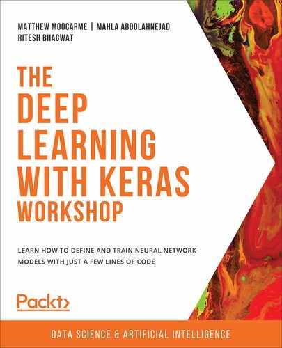
At a high level, such networks that can remember previous states are referred to as recurrent networks. To completely understand RNNs, let's revisit the traditional neural networks, also known as feedforward neural networks. This is a neural network in which the connections of the neural network do not form cycles; that is, the data only flows in one direction, as shown in the following diagram:
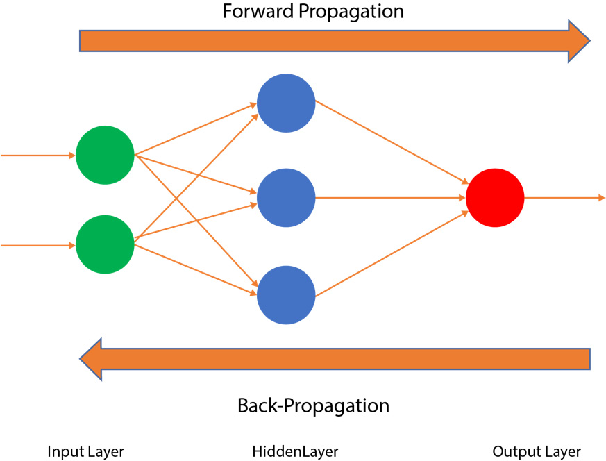
Figure 9.5: A feedforward neural network
In a feedforward neural network, such as the one shown in the preceding diagram, the input layer (the green circles on the left) gets the data and passes it to a hidden layer (with weights, illustrated by the blue circles in the middle). Later, the data from the hidden layer is passed to the output layer (illustrated by the red circle on the right). Based on the thresholds, the data is backpropagated, but there is no cyclical flow of data in the hidden layers.
In an RNN, the hidden layer of the network allows the cycle of data and information. As shown in the following diagram, the architecture is similar to a feedforward neural network; however, here, the data and information also flow in cycles:
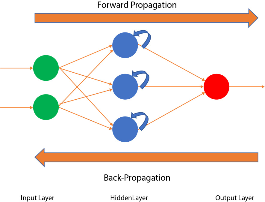
Figure 9.6: An RNN
Here, the defining property of the RNN is that the hidden layer not only gives the output, but it also feeds back the information of the output into itself. Before taking a deep dive into RNNs, let's discuss why we need RNNs and why Convolutional Neural Networks (CNNs) or normal Artificial Neural Networks (ANNs) fall short when it comes to processing sequential data. Suppose that we are using a CNN to identify images; first, we input an image of a dog, and the CNN will label the image as "dog". Then, we input an image of a mango, and the CNN will label the image as "mango". Let's input the image of the dog at time t, as follows:

Figure 9.7: An image of a dog with a CNN
Now, let's input the image of the mango at time t + 1, as follows:
Figure 9.8: An image of a mango with a CNN
Here, you can clearly see that the output at time t for the dog image and the output at time t + 1 for the mango image are totally independent of each other. Therefore, we don't need our algorithms to remember previous instances of the output. However, as we mentioned in the Google Assistant example where we asked when the United Nations was formed and why it was formed, the output of the previous instance has to be remembered by the algorithm for it to process the sequential data. CNNs or ANNs are not able to do this, so we need to use RNNs instead.
In an RNN, we can have multiple outputs over multiple instances of time. The following diagram is a pictorial representation of an RNN. It represents the state of the network from time t – 1 to time t + n:
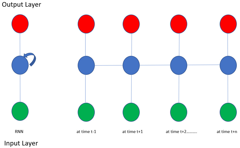
Figure 9.9: An unfolded RNN at various timestamps
There are some issues that you may face when training RNNs that are related to the unique architecture of RNNs. They concern the value of the gradient because, as the depth of the RNN increases, the gradient can either vanish or explode, as we will learn in the next section.
The Vanishing Gradient Problem
If someone asks you "What did you have for dinner last night?", it is pretty easy to remember and correctly answer them. Now, if someone asks you "What did you have for dinner over the past 30 days?", then you might be able to remember the menu of the past 3 or 4 days, but then the menu for the days before that will be a bit difficult to remember. This ability to recall information from the past is the basis of the vanishing gradient problem, which we will be studying in this section. Put simply, the vanishing gradient problem refers to information that is lost or has decayed over a period of time.
The following diagram represents the state of the RNN at different instances of time t. The top dots (in red) represent the output layer, the middle dots (in blue) represent the hidden layer, and the bottom dots (in green) represent the input layer:

Figure: 9.10: Information decaying over time
If you are at t + 10, it will be difficult for you to remember what dinner menu you had at time t (which is 10 days prior to the current day). Additionally, if you are at t + 100, it is likely to be impossible for you to remember your dinner menu prior to 100 days, assuming that there is no pattern to the dinner you choose to make. In the context of machine learning, the vanishing gradient problem is a difficulty that is found when training ANNs using gradient-based learning methods and backpropagation. Let's recall how a neural network works, as follows:
- First, we initialize the network with random weights and bias values.
- We get a predicted output; this output is compared with the actual output and the difference is known as the cost.
- The training process utilizes a gradient, which measures the rate at which the cost changes with respect to the weights or biases.
- Then, we try to lower the cost by adjusting the weights and biases repeatedly throughout the training process, until the lowest possible value is obtained.
For example, if you place a ball on a steep floor, then the ball will roll quickly; however, if you place the ball on a flat surface, it will roll slowly, or not at all. Similarly, in a deep neural network, the model learns quickly when the gradient is large. However, if the gradient is small, then the model's learning rate becomes very low. Remember that, at any point, the gradient is the product of all the gradients up to that point (that is, it follows the calculus chain rule).
Additionally, the gradient is usually a small number between 0 and 1, and the product of two numbers between 0 and 1 gives you an even smaller number. The deeper your network is, the smaller the gradient is in the initial layers of the network. In some cases, it reaches a point that is so small that no training happens in that network; this is the vanishing gradient problem. The following diagram shows the gradients following the calculus chain rule:
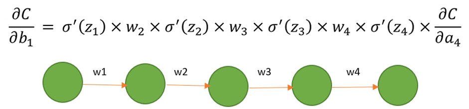
Figure 9.11: The vanishing gradient with cost, C, and the calculus chain rule
Referring to Figure 9.10, suppose that we are at the t + 10 instance and we get an output that will be backpropagated to t, which is 10 steps away. Now, when the weight is updated, there will be 10 gradients (which are themselves very small), and when they multiply by each other, the number becomes so small that it is almost negligible. This is known as the vanishing gradient.
A Brief Explanation of the Exploding Gradient Problem
If instead of the weights being small, the weights are greater than 1, then the subsequent multiplication will increase the gradient exponentially; this is known as the exploding gradient. The exploding gradient is simply the opposite of the vanishing gradient as in the case of the vanishing gradient, the values become too small, while in the case of the exploding gradient, the values become very large. As a result, the network suffers heavily and is unable to predict anything. We don't get the exploding gradient problem as frequently as vanishing gradients, but it is good to have a brief understanding of what exploding gradients are.
There are some approaches we take to overcome the challenges that are faced with the vanishing or exploding gradient problem. The one approach that we will learn about is Long Short-Term Memory, which overcomes issues with the gradients by having memory about information for long periods of time.
Long Short-Term Memory (LSTM)
LSTMs are RNNs whose main objective is to overcome the shortcomings of the vanishing gradient and exploding gradient problems. The architecture is built so that they remember data and information for a long period of time.
LSTMs were designed to overcome the limitation of the vanishing and exploding gradient problems. LSTM networks are a special kind of RNN that are capable of learning long-term dependencies. They are designed to avoid the long-term dependency problem; being able to remember information for long intervals of time is how they are wired. The following diagram displays a standard recurrent network where the repeating module has a tanh activation function. This is a simple RNN. In this architecture, we often have to face the vanishing gradient problem:

Figure 9.12: A simple RNN model
The LSTM architecture is similar to simple RNNs, but their repeating module has different components, as shown in the following diagram:

Figure 9.13: The LSTM model architecture
In addition to a simple RNN, an LSTM consists of the following:
- Sigmoid activation functions (σ)
- Mathematical computational functions (the black circles with + and x)
- Gated cells (or gates):

Figure 9.14: An LSTM in detail
The main difference between a simple RNN and an LSTM is the presence of gated cells. You can think of gates as computer memory, where information can be written, read, or stored. The preceding diagram shows a detailed image of an LSTM. The cells in the gates (represented by the black circles) make decisions on what to store and when to allow values to be read or written. The gates accept any information from 0 to 1; that is, if it is 0, then the information is blocked; if it is 1, then all the information flows through. If the input is between 0 and 1, then only partial information flows.
Besides these input gates, the gradient of a network is dependent on two factors: weight and the activation function. The gates decide which piece of information needs to persist within the LSTM cell and which needs to be forgotten or deleted. In this way, the gates are like water valves; that is, the network can select which valve will allow the water to flow and which valve won't allow the water to flow.
The valves are adjusted in such a way that the values of the output will never yield a gradient (vanishing or exploding) problem. For example, if the value becomes too large, then there is a forget gate that will forget the value and no longer consider it for computations. Essentially, what a forget gate does is multiply the information by 0 or 1. If the information needs to be processed further, then the forget gate multiplies the information by 1, and if it needs to be forgotten, then it multiplies the information by 0. Each gate is assisted by a sigmoid function that squashes the information between 0 and 1. For us to gain a better understanding of this, let's take a look at some activities and exercises.
Note
All the activities and exercises in this chapter will be developed in Jupyter notebooks. You can download this book's GitHub repository, along with all the prepared templates, at https://packt.live/2vtdA8o.
Exercise 9.01: Predicting the Trend of Alphabet's Stock Price Using an LSTM with 50 Units (Neurons)
In this exercise, we will examine the stock price of Alphabet over a period of 5 years—that is, from January 1, 2014, to December 31, 2018. In doing so, we will try to predict and forecast the company's future trend for January 2019 using RNNs. We have the actual values for January 2019, so we will be able to compare our predictions with the actual values later. Follow these steps to complete this exercise:
- Import the required libraries:
import numpy as np
import matplotlib.pyplot as plt
import pandas as pd
from tensorflow import random
- Import the dataset using the pandas read_csv function and look at the first five rows of the dataset using the head method:
dataset_training = pd.read_csv('../GOOG_train.csv')
dataset_training.head()
The following figure shows the output of the preceding code:
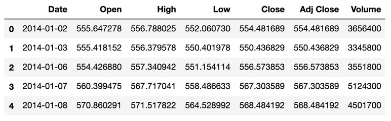
Figure 9.15: The first five rows of the GOOG_Training dataset
- We are going to make our prediction using the Open stock price; therefore, select the Open stock price column from the dataset and print the values:
training_data = dataset_training[['Open']].values
training_data
The preceding code produces the following output:
array([[ 555.647278],
[ 555.418152],
[ 554.42688 ],
...,
[1017.150024],
[1049.619995],
[1050.959961]])
- Then, perform feature scaling by normalizing the data using MinMaxScaler and setting the range of the features so that they have a minimum value of 0 and a maximum value of one. Use the fit_transform method of the scaler on the training data:
from sklearn.preprocessing import MinMaxScaler
sc = MinMaxScaler(feature_range = (0, 1))
training_data_scaled = sc.fit_transform(training_data)
training_data_scaled
The preceding code produces the following output:
array([[0.08017394],
[0.07987932],
[0.07860471],
...,
[0.67359064],
[0.71534169],
[0.71706467]])
- Create the data to get 60 timestamps from the current instance. We chose 60 here as this will give us a sufficient number of previous instances so that we can understand the trend; technically, this can be any number, but 60 is the optimal value. Additionally, the upper bound value here is 1258, which is the index or count of rows (or records) in the training set:
X_train = []
y_train = []
for i in range(60, 1258):
X_train.append(training_data_scaled[i-60:i, 0])
y_train.append(training_data_scaled[i, 0])
X_train, y_train = np.array(X_train),
np.array(y_train)
- Next, reshape the data to add an extra dimension to the end of X_train using NumPy's reshape function:
X_train = np.reshape(X_train, (X_train.shape[0],
X_train.shape[1], 1))
X_train
The following figure shows the output of the preceding code:

Figure 9.16: The data of a few timestamps from the current instance
- Import the following Keras libraries to build the RNN:
from keras.models import Sequential
from keras.layers import Dense, LSTM, Dropout
- Set the seed and initiate the sequential model, as follows:
seed = 1
np.random.seed(seed)
random.set_seed(seed)
model = Sequential()
- Add an LSTM layer to the network with 50 units, set the return_sequences argument to True, and set the input_shape argument to (X_train.shape[1], 1). Add three additional LSTM layers, each with 50 units, and set the return_sequences argument to True for the first two, as follows:
model.add(LSTM(units = 50, return_sequences = True,
input_shape = (X_train.shape[1], 1)))
# Adding a second LSTM layer
model.add(LSTM(units = 50, return_sequences = True))
# Adding a third LSTM layer
model.add(LSTM(units = 50, return_sequences = True))
# Adding a fourth LSTM layer
model.add(LSTM(units = 50))
# Adding the output layer
model.add(Dense(units = 1))
- Compile the network with an adam optimizer and use Mean Squared Error for the loss. Fit the model to the training data for 100 epochs with a batch size of 32:
# Compiling the RNN
model.compile(optimizer = 'adam', loss = 'mean_squared_error')
# Fitting the RNN to the Training set
model.fit(X_train, y_train, epochs = 100, batch_size = 32)
- Load and process the test data (which is treated as actual data here) and select the column representing the value of Open stock data:
dataset_testing = pd.read_csv("../GOOG_test.csv")
actual_stock_price = dataset_testing[['Open']].values
actual_stock_price
The following figure shows the output of the preceding code:

Figure 9.17: The actual processed data
- Concatenate the data; we will need 60 previous instances in order to get the stock price for each day. Therefore, we will need both training and test data:
total_data = pd.concat((dataset_training['Open'],
dataset_testing['Open']), axis = 0)
- Reshape and scale the input to prepare the test data. Note that we are predicting the January monthly trend, which has 21 financial days, so in order to prepare the test set, we take the lower bound value as 60 and the upper bound value as 81. This ensures that the difference of 21 is maintained:
inputs = total_data[len(total_data)
- len(dataset_testing) - 60:].values
inputs = inputs.reshape(-1,1)
inputs = sc.transform(inputs)
X_test = []
for i in range(60, 81):
X_test.append(inputs[i-60:i, 0])
X_test = np.array(X_test)
X_test = np.reshape(X_test, (X_test.shape[0],
X_test.shape[1], 1))
predicted_stock_price = model.predict(X_test)
predicted_stock_price = sc.inverse_transform(
predicted_stock_price)
- Visualize the results by plotting the actual stock price and then plotting the predicted stock price:
# Visualizing the results
plt.plot(actual_stock_price, color = 'green',
label = 'Real Alphabet Stock Price',
ls='--')
plt.plot(predicted_stock_price, color = 'red',
label = 'Predicted Alphabet Stock Price',
ls='-')
plt.title('Predicted Stock Price')
plt.xlabel('Time in days')
plt.ylabel('Real Stock Price')
plt.legend()
plt.show()
Please note that your results may differ slightly to the actual stock price of Alphabet.
Expected output:
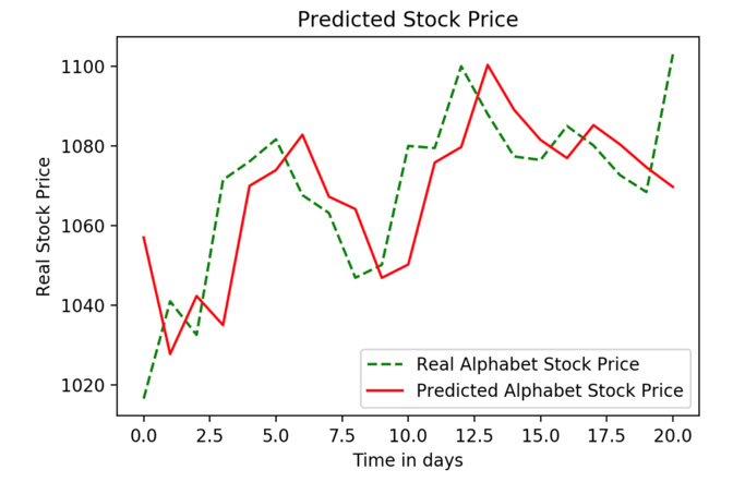
Figure 9.18: The real versus predicted stock price
This concludes Exercise 9.01, Predicting the Trend of Alphabet's Stock Price Using an LSTM with 50 Units (Neurons), where we have predicted Alphabet's stock trends with the help of an LSTM. As shown in the preceding plot, the trend has been captured fairly.
Note
To access the source code for this specific section, please refer to https://packt.live/2ZwdAzW.
You can also run this example online at https://packt.live/2YV3PvX.
In the next activity, we will test our knowledge and practice building RNNs with LSTM layers by predicting the trend of Amazon's stock price over the last 5 years.
Activity 9.01: Predicting the Trend of Amazon's Stock Price Using an LSTM with 50 Units (Neurons)
In this activity, we will examine the stock price of Amazon for the last 5 years—that is, from January 1, 2014, to December 31, 2018. In doing so, we will try to predict and forecast the company's future trend for January 2019 using an RNN and LSTM. We have the actual values for January 2019, so we can compare our predictions to the actual values later. Follow these steps to complete this activity:
- Import the required libraries.
- From the full dataset, extract the Open column as the predictions will be made on the open stock value. Download the dataset from this book's GitHub repository. You can find the dataset at https://packt.live/2vtdA8o.
- Normalize the data between 0 and 1.
- Then, create timestamps. The values of each day in January 2019 will be predicted by the previous 60 days; so, if January 1 is predicted by using the value from the nth day up to December 31, then January 2 will be predicted by using the n + 1st day and January 1, and so on.
- Reshape the data into three dimensions since the network needs data in three dimensions.
- Build an RNN model in Keras using 50 units (here, units refer to neurons) with four LSTM layers. The first step should provide the input shape. Note that the final LSTM layer always adds return_sequences=True, so it doesn't have to be explicitly defined.
- Process and prepare the test data that is the actual data for January 2019.
- Combine and process the training and test data.
- Visualize the results.
After implementing these steps, you should see the following expected output:
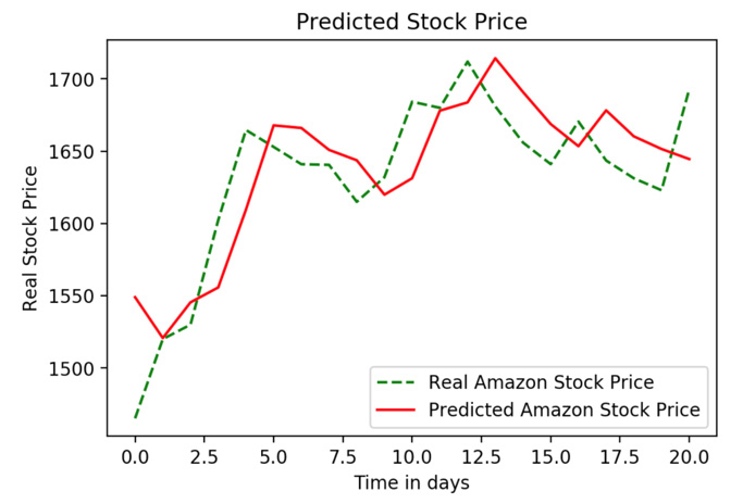
Figure 9.19: Real versus predicted stock prices
Note
The solution for this activity can be found on page 452.
Now, let's try and improve performance by tweaking our LSTM. There is no gold standard on how to build an LSTM; however, the following permutation combinations can be tried in order to improve performance:
- Build an LSTM with moderate units, such as 50
- Build an LSTM with over 100 units
- Use more data; that is, instead of 5 years, take data from 10 years
- Apply regularization using 100 units
- Apply regularization using 50 units
- Apply regularization using more data and 50 units
This list can have a number of combinations; whichever combination offers the best results can be considered a good algorithm for that particular dataset. In the next exercise, we will explore one of these options by adding more units to our LSTM layer and observing the performance.
Exercise 9.02: Predicting the Trend of Alphabet's Stock Price Using an LSTM with 100 units
In this exercise, we will examine the stock price of Alphabet over the last 5 years, from January 1, 2014, to December 31, 2018. In doing so, we will try to predict and forecast the company's future trend for January 2019 using RNNs. We have the actual values for January 2019, so we will compare our predictions with the actual values later. This is the same task as the first exercise, but now we're using 100 units instead. Make sure that you compare the output with Exercise 9.01, Predicting the Trend of Alphabet's Stock Price Using an LSTM with 50 Units (Neurons). Follow these steps to complete this exercise:
- Import the required libraries:
import numpy as np
import matplotlib.pyplot as plt
import pandas as pd
from tensorflow import random
- Import the dataset using the pandas read_csv function and look at the first five rows of the dataset using the head method:
dataset_training = pd.read_csv('../GOOG_train.csv')
dataset_training.head()
- We are going to make our prediction using the Open stock price; therefore, select the Open stock price column from the dataset and print the values:
training_data = dataset_training[['Open']].values
training_data
- Then, perform feature scaling by normalizing the data using MinMaxScaler and setting the range of the features so that they have a minimum value of zero and a maximum value of one. Use the fit_transform method of the scaler on the training data:
from sklearn.preprocessing import MinMaxScaler
sc = MinMaxScaler(feature_range = (0, 1))
training_data_scaled = sc.fit_transform(training_data)
training_data_scaled
- Create the data to get 60 timestamps from the current instance. We chose 60 here as it will give us a sufficient number of previous instances in order to understand the trend; technically, this can be any number, but 60 is the optimal value. Additionally, the upper bound value here is 1258, which is the index or count of rows (or records) in the training set:
X_train = []
y_train = []
for i in range(60, 1258):
X_train.append(training_data_scaled[i-60:i, 0])
y_train.append(training_data_scaled[i, 0])
X_train, y_train = np.array(X_train), np.array(y_train)
- Reshape the data to add an extra dimension to the end of X_train using NumPy's reshape function:
X_train = np.reshape(X_train, (X_train.shape[0],
X_train.shape[1], 1))
- Import the following Keras libraries to build the RNN:
from keras.models import Sequential
from keras.layers import Dense, LSTM, Dropout
- Set the seed and initiate the sequential model, as follows:
seed = 1
np.random.seed(seed)
random.set_seed(seed)
model = Sequential()
- Add an LSTM layer to the network with 50 units, set the return_sequences argument to True, and set the input_shape argument to (X_train.shape[1], 1). Add three additional LSTM layers, each with 50 units, and set the return_sequences argument to True for the first two. Add a final output layer of size 1:
model.add(LSTM(units = 100, return_sequences = True,
input_shape = (X_train.shape[1], 1)))
# Adding a second LSTM
model.add(LSTM(units = 100, return_sequences = True))
# Adding a third LSTM layer
model.add(LSTM(units = 100, return_sequences = True))
# Adding a fourth LSTM layer
model.add(LSTM(units = 100))
# Adding the output layer
model.add(Dense(units = 1))
- Compile the network with an adam optimizer and use Mean Squared Error for the loss. Fit the model to the training data for 100 epochs with a batch size of 32:
# Compiling the RNN
model.compile(optimizer = 'adam', loss = 'mean_squared_error')
# Fitting the RNN to the Training set
model.fit(X_train, y_train, epochs = 100, batch_size = 32)
- Load and process the test data (which is treated as actual data here) and select the column representing the value of Open stock data:
dataset_testing = pd.read_csv("../GOOG_test.csv")
actual_stock_price = dataset_testing[['Open']].values
actual_stock_price
- Concatenate the data since we will need 60 previous instances to get the stock price for each day. Therefore, we will need both the training and test data:
total_data = pd.concat((dataset_training['Open'],
dataset_testing['Open']), axis = 0)
- Reshape and scale the input to prepare the test data. Note that we are predicting the January monthly trend, which has 21 financial days, so in order to prepare the test set, we take the lower bound value as 60 and the upper bound value as 81. This ensures that the difference of 21 is maintained:
inputs = total_data[len(total_data)
- len(dataset_testing) - 60:].values
inputs = inputs.reshape(-1,1)
inputs = sc.transform(inputs)
X_test = []
for i in range(60, 81):
X_test.append(inputs[i-60:i, 0])
X_test = np.array(X_test)
X_test = np.reshape(X_test, (X_test.shape[0],
X_test.shape[1], 1))
predicted_stock_price = model.predict(X_test)
predicted_stock_price = sc.inverse_transform(
predicted_stock_price)
- Visualize the results by plotting the actual stock price and plotting the predicted stock price:
# Visualizing the results
plt.plot(actual_stock_price, color = 'green',
label = 'Real Alphabet Stock Price',ls='--')
plt.plot(predicted_stock_price, color = 'red',
label = 'Predicted Alphabet Stock Price',ls='-')
plt.title('Predicted Stock Price')
plt.xlabel('Time in days')
plt.ylabel('Real Stock Price')
plt.legend()
plt.show()
Expected output:
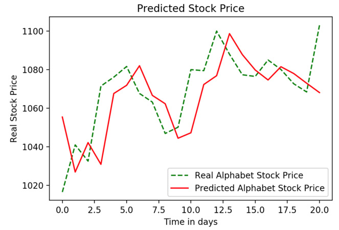
Figure 9.20: Real versus predicted stock price
Note
To access the source code for this specific section, please refer to https://packt.live/2ZDggf4.
You can also run this example online at https://packt.live/2O4ZoJ7.
Now, if we compare the LSTM of Exercise 9.01, Predicting the Trend of Alphabet's Stock Price Using an LSTM with 50 Units (Neurons), which had 50 neurons (units), with this LSTM, which uses 100 units, we can see that, unlike in the case of the Amazon stock price, the Alphabet stock trend is captured better using an LSTM with 100 units:

Figure 9.21: Comparing the output with the LSTM of Exercise 9.01
Thus, we can clearly see that an LSTM with 100 units predicts a more accurate trend than an LSTM with 50 units. Do keep in mind that an LSTM with 100 units will need more computational time but provides better results in this scenario. As well as modifying our model by adding more units, we can also add regularization. The following activity will test whether adding regularization can make our Amazon model more accurate.
Activity 9.02: Predicting Amazon's Stock Price with Added Regularization
In this activity, we will examine the stock price of Amazon over the last 5 years, from January 1, 2014, to December 31, 2018. In doing so, we will try to predict and forecast the company's future trend for January 2019 using RNNs and an LSTM. We have the actual values for January 2019, so we will be able to compare our predictions with the actual values later. Initially, we predicted the trend of Amazon's stock price using an LSTM with 50 units (or neurons). Here, we will also add dropout regularization and compare the results with Activity 9.01, Predicting the Trend of Amazon's Stock Price Using an LSTM with 50 Units (Neurons). Follow these steps to complete this activity:
- Import the required libraries.
- From the full dataset, extract the Open column since the predictions will be made on the open stock value. You can download the dataset from this book's GitHub repository at https://packt.live/2vtdA8o.
- Normalize the data between 0 and 1.
- Then, create timestamps. The values of each day in January 2019 will be predicted by the previous 60 days. So, if January 1 is predicted by using the value from the nth day up to December 31, then January 2 will be predicted by using the n + 1st day and January 1, and so on.
- Reshape the data into three dimensions since the network needs the data to be in three dimensions.
- Build an RNN with four LSTM layers in Keras, each with 50 units (here, units refer to neurons), and a 20% dropout after each LSTM layer. The first step should provide the input shape. Note that the final LSTM layer always adds return_sequences=True.
- Process and prepare the test data, which is the actual data for January 2019.
- Combine and process the train and test data.
- Finally, visualize the results.
After implementing these steps, you should get the following expected output:

Figure 9.22: Real versus predicted stock prices
Note
The solution for this activity can be found on page 457.
In the next activity, we will experiment with building an RNN with 100 units in each LSTM layer and compare this with how the RNN performed with only 50 units.
Activity 9.03: Predicting the Trend of Amazon's Stock Price Using an LSTM with an Increasing Number of LSTM Neurons (100 Units)
In this activity, we will examine the stock price of Amazon over the last 5 years, from January 1, 2014, to December 31, 2018. In doing so, we will try to predict and forecast the company's future trend for January 2019 using RNNs. We have the actual values for January 2019, so we will be able to compare our predictions with the actual values later. You can also compare the output difference with Activity 9.01, Predicting the Trend of Amazon's Stock Price Using an LSTM with 50 Units (Neurons). Follow these steps to complete this activity:
- Import the required libraries.
- From the full dataset, extract the Open column since the predictions will be made on the Open stock value.
- Normalize the data between 0 and 1.
- Then, create timestamps. The values of each day in January 2019 will be predicted by the previous 60 days; so, if January 1 is predicted by using the value from the nth day up to December 31, then January 2 will be predicted by using the n + 1st day and January 1, and so on.
- Reshape the data into three dimensions since the network needs data to be in three dimensions.
- Build an LSTM in Keras with 100 units (here, units refer to neurons). The first step should provide the input shape. Note that the final LSTM layer always adds return_sequences=True. Compile and fit the model to the training data.
- Process and prepare the test data, which is the actual data for January 2019.
- Combine and process the training and test data.
- Visualize the results.
After implementing these steps, you should get the following expected output:

Figure 9.23: Real versus predicted stock prices
Note
The solution for this activity can be found on page 462.
In this activity, we created an RNN with four LSTM layers, each with 100 units. We compared this to the results of Activity 9.02, Predicting Amazon's Stock Price with Added Regularization, in which there were 50 units per layer. The difference between the two models was minimal, so a model with fewer units is preferable due to the decrease in computational time and there being a smaller possibility of overfitting the training data.
Summary
In this chapter, we learned about sequential modeling and sequential memory by examining some real-life cases with Google Assistant. Then, we learned how sequential modeling is related to RNNs, as well as how RNNs are different from traditional feedforward networks. We learned about the vanishing gradient problem in detail and how using an LSTM is better than a simple RNN to overcome the vanishing gradient problem. We applied what we learned to time series problems by predicting stock trends.
In this workshop, we learned the basics of machine learning and Python, while also gaining an in-depth understanding of applying Keras to develop efficient deep learning solutions. We explored the difference between machine and deep learning. We began the workshop by building a logistic regression model, first with scikit-learn, and then with Keras.
Then, we explored Keras and its different models further by creating prediction models for various real-world scenarios, such as classifying online shoppers into those with purchase intention and those without. We learned how to evaluate, optimize, and improve models to achieve maximum information to create robust models that perform well on new, unseen data.
We also incorporated cross-validation by building Keras models with wrappers for scikit-learn that help those familiar with scikit-learn workstreams utilize Keras models easily. Then, we learned how to apply L1, L2, and dropout regularization techniques to improve the accuracy of models and to help prevent our models from overfitting the training data.
Next, we explored model evaluation further by applying techniques such as null accuracy for baseline comparison and evaluation metrics such as precision, the AUC-ROC score, and more to understand how our model scores classification tasks. Ultimately, these advanced evaluation techniques helped us understand under what conditions our model is performing well and where there is room for improvement.
We ended the workshop by creating some advanced models with Keras. We explored computer vision by building CNN models with various parameters to classify images. Then, we used pre-trained models to classify new images and fine-tuned those pre-trained models so that we could utilize them for our own applications. Finally, we covered sequential modeling, which is used for modeling sequences such as stock prices and natural language processing. We tested this knowledge by creating RNN networks with LSTM layers to predict the stock price of real stock data and experimented with various numbers of units in each layer and the effect of dropout regularization on the model's performance.
Overall, we have gained a comprehensive understanding of how to use Keras to solve a variety of problems using real-world datasets. We covered the classification tasks of online shoppers, hepatitis C data, and failure data for Scania trucks, as well as regression tasks such as predicting the aquatic toxicity of various chemicals when given various chemical attributes. We also performed image classification tasks and built CNN models to predict whether images are of flowers or cars, and also built regression tasks to predict future stock prices with RNNs. By using this workshop to build models with real-word datasets, you are ready to apply your learning and understanding to your own problem-solving and create your own applications.