Overview
In this chapter, you will experiment with different neural network architectures. You will create Keras sequential models—building single-layer and multi-layer models—and evaluate the performance of trained models. Networks of different architectures will help you understand overfitting and underfitting. By the end of this chapter, you will have explored early stopping that can be used to combat overfitting to the training data.
Introduction
In the previous chapter, you learned about the mathematics of neural networks, including linear transformations with scalars, vectors, matrices, and tensors. Then, you implemented your first neural network using Keras by building a logistic regression model to classify users of a website into those who will purchase from the website and those who will not.
In this chapter, you will extend your knowledge of building neural networks using Keras. This chapter covers the basics of deep learning and will provide you with the necessary foundations so that you can build highly complex neural network architectures. We will start by extending the logistic regression model to a simple single-layer neural network and then proceed to more complicated neural networks with multiple hidden layers.
In this process, you will learn about the underlying basic concepts of neural networks, including forward propagation for making predictions, computing loss, backpropagation for computing derivatives of loss with respect to model parameters, and, finally, gradient descent for learning about optimal parameters for the model. You will also learn about the various choices that are available so that you can build and train a neural network in terms of activation functions, loss functions, and optimizers.
Furthermore, you will learn how to evaluate your model while understanding issues such as overfitting and underfitting, all while looking at how they can impact the performance of your model and how to detect them. You will learn about the drawbacks of evaluating a model on the same dataset that's used for training, as well as the alternative approach of holding back a part of the available dataset for evaluation purposes. Subsequently, you will learn how to compare the model error rate on each of these two subsets of the dataset that can be used to detect problems such as high bias and high variance in the model. Lastly, you will learn about a technique called early stopping to reduce overfitting, which is again based on comparing the model's error rate to the two subsets of the dataset.
Building Your First Neural Network
In this section, you will learn about the representations and concepts of deep learning, such as forward propagation—the propagation of data through the network, multiplying the input values by the weight of each connection for every node, and backpropagation—the calculation of the gradient of the loss function with respect to the weights in the matrix, and gradient descent—the optimization algorithm that's used to find the minimum of the loss function.
We will not delve deeply into these concepts as it isn't required for this book. However, this coverage will essentially help anyone who wants to apply deep learning to a problem.
Then, we will move on to implementing neural networks using Keras. Also, we will stick to the simplest case, which is a neural network with a single hidden layer. You will learn how to define a model in Keras, choose the hyperparameters—the parameters of the model that are set before training the model—and then train your model. At the end of this section, you will have the opportunity to practice what you have learned by implementing a neural network in Keras so that you can perform classification on a dataset and observe how neural networks outperform simpler models such as logistic regression.
Logistic Regression to a Deep Neural Network
In Chapter 1, Introduction to Machine Learning with Keras, you learned about the logistic regression model, and then how to implement it as a sequential model using Keras in Chapter 2, Machine Learning versus Deep Learning. Technically speaking, logistic regression involves a very simple neural network with only one hidden layer and only one node in its hidden layer.
An overview of the logistic regression model with two-dimensional input can be seen in the following image. What you see in this image is called one node or unit in the deep learning world, which is represented by the green circle. As you may have noticed, there are some differences between logistic regression terminology and deep learning terminology. In logistic regression, we call the parameters of the model coefficients and intercepts. In deep learning models, the parameters are referred to as weights (w) and biases (b):

Figure 3.1: Overview of the logistic regression model with a two-dimensional input
At each node/unit, the inputs are multiplied by some weights and then a bias term is added to the sum of these weighted inputs. This can be seen in the calculation above the node in the preceding image. The inputs are X1 and X2, the weights are W1 and W2, and the bias is b. Next, a nonlinear function (for example, a sigmoid function in the case of a logistic regression model) is applied to the sum of the weighted inputs and the bias term is used to compute the final output of the node. In the calculation shown in the preceding image, this is σ. In deep learning, the nonlinear function is called the activation function and the output of the node is called the activation of that node.
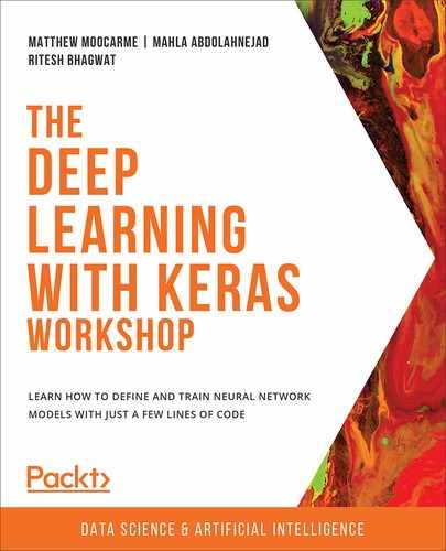
It is possible to build a single-layer neural network by stacking logistic regression nodes/units on top of each other in a layer, as shown in the following image. Every value at the input layers, X1 and X2, is passed to all three nodes at the hidden layer:
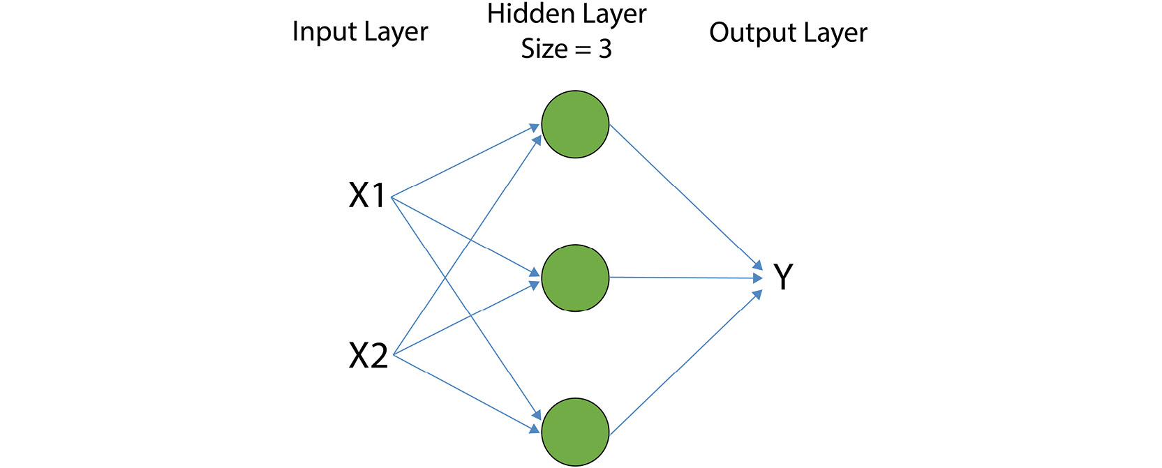
Figure 3.2: Overview of a single-layer neural network with a two-dimensional input and a hidden layer of size 3
It is also possible to build multi-layer neural networks by stacking multiple layers of processing nodes after one another, as shown in the following image. The following image shows a two-layer neural network with two-dimensional input:

Figure 3.3: Overview of a two-layer neural network with a two-dimensional input
The preceding two images show the most common way of representing a neural network. Every neural network consists of an input layer, an output layer, and one or many hidden layers. If there is only one hidden layer, the network is called a shallow neural network. On the other hand, neural networks with many hidden layers are called deep neural networks, and the process of training them is called deep learning.
Figure 3.2 shows a neural network with only one hidden layer, so this would be a shallow neural network, whereas the neural network in Figure 3.3 has two hidden layers, so it is a deep neural network. The input layers are generally on the left. In the case of Figure 3.3, these are features X1 and X2, and they are input into the first hidden layer, which has three nodes. The arrows represent the weight values that are applied to the input. At the second hidden layer, the result of the first hidden layer becomes the input to the second hidden layer. The arrows between the first and second hidden layers represent the weights. The output is generally the layer on the far right and, in the case of Figure 3.3, is represented by the layer labeled Y.
Note
In some resources, you may see that a network, such as the one shown in the preceding image, is referred to as a four-layer network. This is because the input and output layers are counted along with the hidden layers. However, the more common convention is to count only the hidden layers, so the network we mentioned previously will be referred to as a two-layer network.
In a deep learning setting, the number of nodes in the input layer is equal to the number of features of the input data, and the number of nodes in the output layer is equal to the number of dimensions of the output data. However, you need to select the number of nodes in the hidden layers or the size of the hidden layers. If you choose a larger size layer, the model becomes more flexible and will be able to model more complex functions. This increase in flexibility comes at the cost of the need for more training data and more computations to train the model on. The parameters that are required to be selected by the developer are called hyperparameters and include parameters such as the number of layers and the number of nodes in each layer. Common hyperparameters to be chosen include the number of epochs to train for and the loss function to use.
In the next section, we will cover activation functions that are applied after each hidden layer.
Activation Functions
In addition to the size of the layer, you need to choose an activation function for each hidden layer that you add to the model, and also do the same for the output layer. We learned about the sigmoid activation function in the logistic regression model. However, there are more options for activation functions that you can choose from when building a neural network in Keras. For example, the sigmoid activation function is a good choice as the activation function on the output layer for binary classification tasks since the result of a sigmoid function is bounded between 0 and 1. Some commonly used activation functions for deep learning are sigmoid/logistic, tanh (hyperbolic tangent), and Rectified Linear Unit (ReLU).
The following image shows a sigmoid activation function:

Figure 3.4: Sigmoid activation function
The following image shows a tanh activation function:

Figure 3.5: tanh activation function
The following image shows a ReLU activation function:

Figure 3.6: ReLU activation function
As you can see in Figures 3.4 and 3.5, the output of a sigmoid function is always between 0 and 1, and the output of tanh is always between -1 and 1. This makes tanh a better choice for hidden layers since it keeps the average of the outputs in each layer close to zero. In fact, sigmoid is only a good choice for the activation function of the output layer when building a binary classifier since its output can be interpreted as the probability of a given input belonging to one class.
Therefore, tanh and ReLU are the most common choices of activation function for hidden layers. It turns out that the learning process is faster when using the ReLU activation function because it has a fixed derivative (or slope) for an input greater than 0, and a slope of 0 everywhere else.
Note
You can read more about all the available choices for activation functions in Keras here: https://keras.io/activations/.
Forward Propagation for Making Predictions
Neural networks make a prediction about the output by performing forward propagation. Forward propagation entails the computations that are performed on the input in every layer of a neural network until the output layer is reached. It is best to understand forward propagation through an example.
Let's go through forward propagation equations one by one for a two-layer neural network (shown in the following image) where the input data is two-dimensional, and the output data is a one-dimensional binary class label. The activation functions for layer 1 and layer 2 will be tanh, and the activation function in the output layer is sigmoid.
The following image shows the weights and biases for each layer as matrices and vectors with proper indexes. For each layer, the number of rows in the weight's matrix is equal to the number of nodes in the previous layer, and the number of columns is equal to the number of nodes in that layer.
For example, W1 has two rows and three columns because the input to layer 1 is the input layer, X, which has two columns, and layer 1 has three nodes. Likewise, W2 has three rows and three columns because the input to layer 2 is layer 1, which has two nodes, and layer 2 has five nodes. The bias, however, is always a vector with a size equal to the number of nodes in that layer. The total number of parameters in a deep learning model is equal to the total number of elements in all the weights' matrices and the biases' vectors:

Figure 3.7: A two-layer neural network
An example of performing all the steps for forward propagation according to the neural network outlined in the preceding image is as follows.
Steps to perform forward propagation:
- X is the network input to the network in the preceding image, so it is the input for the first hidden layer. First, the input matrix, X, is the matrix multiplied by the weight matrix for layer 1, W1, and the bias, b1, is added:
z1 = X*W1 + b1
- Next, the layer 1 output is computed by applying an activation function to z1, which is the output of the previous step:
a1 = tanh(z1)
- a1 is the output of layer 1 and is called the activation of layer 1. The output of layer 1 is, in fact, the input for layer 2. Next, the activation of layer 1 is the matrix multiplied by the weight matrix for layer 2, W2, and the bias, b2, is added:
z2 = a1 * W2 + b2
- The layer 2 output/activation is computed by applying an activation function to z2:
a2 = tanh(z2)
- The output of layer 2 is, in fact, the input for the next layer (the network output layer here). Following this, the activation of layer 2 is the matrix multiplied by the weight matrix for the output layer, W3, and the bias, b3, is added:
z3 = a2 * W3 + b3
- Finally, the network output, Y, is computed by applying the sigmoid activation function to z3:
Y = sigmoid(z3)
The total number of parameters in this model is equal to the sum of the number of elements in W1, W2, W3, b1, b2, and b3. Therefore, the number of parameters can be calculated by summing the parameters in each of the parameters in weight matrices and biases, which is equal to 6 + 15 + 5 + 3 + 5 + 1 = 35. These are the parameters that need to be learned in the process of deep learning.
Now that we have learned about the forward propagation step, we have to evaluate our model and compare it to the real target values. To achieve that, we will use a loss function, which we will cover in the next section. Here, we will learn about some common loss functions that we can use for classification and regression tasks.
Loss Function
When learning the optimal parameters (weights and biases) of a model, we need to define a function to measure error. This function is called the loss function and it provides us with a measure of how different network-predicted outputs are from the real outputs in the dataset.
The loss function can be defined in several different ways, depending on the problem and the goal. For example, in the case of a classification problem, one common way to define loss is to compute the proportion of misclassified inputs in the dataset and use that as the probability of the model making an error. On the other hand, in the case of a regression problem, the loss function is usually defined by computing the distance between the predicted outputs and their corresponding real outputs, and then averaging over all the examples in the dataset.
Brief descriptions of some commonly used loss functions that are available in Keras are as follows:
- mean_squared_error is a loss function for regression problems that calculates (real output – predicted output)^2 for each example in the dataset and then returns their average.
- mean_absolute_error is a loss function for regression problems that calculates abs (real output – predicted output) for each example in the dataset and then returns their average.
- mean_absolute_percentage_error is a loss function for regression problems that calculates abs [(real output – predicted output) / real output] for each example in the dataset and then returns their average, multiplied by 100%.
- binary_crossentropy is a loss function for two-class/binary classification problems. In general, the cross-entropy loss is used for calculating the loss for models where the output is a probability number between 0 and 1.
- categorical_crossentropy is a loss function for multi-class (more than two classes) classification problems.
Note
You can read more about all the available choices for loss functions in Keras here: https://keras.io/losses/.
During the training process, we keep changing the model parameters until the minimum difference between the model-predicted outputs and the real outputs is reached. This is called an optimization process, and we will learn more about how it works in later sections. For neural networks, we use backpropagation to compute the derivatives of the loss function with respect to the weights.
Backpropagation for Computing Derivatives of Loss Function
Backpropagation is the process of performing the chain rule of calculus from the output layer to the input layer of a neural network in order to compute the derivatives of the loss function with respect to the model parameters in each layer. The derivative of a function is simply the slope of that function. We are interested in the slope of the loss function because it provides us with the direction in which model parameters need to change in order for the loss value to be minimized.
The chain rule of calculus states that if, for example, z is a function of y, and y is a function of x, then the derivative of z with respect to x can be reached by multiplying the derivative of z with respect to y by the derivative of y with respect to x. This can be written as follows:
dz/dx = dz/dy * dy/dx
In deep neural networks, the loss function is a function of predicted outputs. We can show this through the equation given here:
loss = L(y_predicted)
On the other hand, according to forward propagation equations, the output predicted by the model is a function of the model parameters—that is, the weights and biases in each layer. Therefore, according to the chain rule of calculus, the derivative of the loss with respect to the model parameters can be computed by multiplying the derivative of the loss with respect to the predicted output by the derivative of the predicted output with respect to the model parameters.
In the next section, we will learn how the optimal weight parameters are modified when given the derivatives of the loss function with respect to the weights.
Gradient Descent for Learning Parameters
In this section, we will learn how a deep learning model learns its optimal parameters. Our goal is to update the weight parameters so that the loss function is minimized. This will be an iterative process in which we continue to update the weight parameters so that the loss function is at a minimum. This process is called learning parameters and it is done through the use of an optimization algorithm. One very common optimization algorithm that's used for learning parameters in machine learning is gradient descent. Let's see how gradient descent works.
If we plot the average of loss over all the examples in the dataset for all the possible values of the model parameters, it is usually a convex shape (such as the one shown in the following plot). In gradient descent, our goal is to find the minimum point (Pt) on the plot. The algorithm starts by initializing the model parameters with some random values (P1). Then, it computes the loss and the derivatives of the loss with respect to the parameters at that point. As we mentioned previously, the derivative of a function is, in fact, the slope of the function. After computing the slope at an initial point, we have the direction in which we need to update the parameters.
The hyperparameter, called the learning rate (alpha), determines how big a step the algorithm will take from the initial point. After selecting the proper alpha value, the algorithm updates the parameters from their initial values to the new values (shown as point P2 in the following plot). As shown in the following plot, P2 is closer to the target point, and if we keep moving in that direction, we will eventually get to the target point, Pt. The algorithm computes the slope of the function again at P2 and takes another step.
This process is repeated until the slope is equal to zero and therefore no direction for further movement is provided:

Figure 3.8: A schematic view of the gradient descent algorithm finding the set of parameters that minimize loss
The pseudocode for the gradient descent algorithm is provided here:
Initialize all the weights (w) and biases (b) arbitrarily
Repeat Until converge {
Compute loss given w and b
Compute derivatives of loss with respect to w (dw), and with respect to b (db) using backpropagation
Update w to w – alpha * dw
Update b to b – alpha * db
}
To summarize, the following steps are repeated when training a deep neural network (after initializing the parameters to some random values):
- Use forward propagation and the current parameters to predict the outputs for the entire dataset.
- Use the predicted outputs to compute the loss over all the examples.
- Use backpropagation to compute the derivatives of the loss with respect to the weights and biases at each layer.
- Update the weights and biases using the derivative values and the learning rate.
What we discussed here was the standard gradient descent algorithm, which computes the loss and the derivatives using the entire dataset in order to update the parameters. There is another version of gradient descent called stochastic gradient descent (SGD), which computes the loss and the derivatives each time using a subset or a batch of data examples only; therefore, its learning process is faster than standard gradient descent.
Note
Another common choice is an optimization algorithm called Adam. Adam usually outperforms SGD when training deep learning models. As we've already learned, SGD uses a single hyperparameter (called a learning rate) to update the parameters. However, Adam improves this process by using a learning rate, a weighted average of gradients, and a weighted average of squared gradients to update the parameters at each iteration.
Usually, when building a neural network, you need to choose two hyperparameters (called the batch size and the number of epochs) for your optimization process. The batch_size argument determines the number of data examples to be included at each iteration of the optimization algorithm. batch_size=None is equivalent to the standard version of gradient descent, which uses the entire dataset in each iteration. The epochs argument determines how many times the optimization algorithm passes through the entire training dataset before it stops.
For example, imagine we have a dataset of size n=400, and we choose batch_size=5 and epochs=20. In this case, the optimizer will have 400/5 = 80 iterations in one pass through the entire dataset. Since it is supposed to go through the entire dataset 20 times, it will have 80 * 20 iterations in total.
Note
When building a model in Keras, you need to choose the type of optimizer to be used when training your model. There are some other options other than SGD and Adam available in Keras. You can read more about all the possible options for optimizers in Keras here: https://keras.io/optimizers/.
Note
All the activities and exercises in this chapter will be developed in a Jupyter notebook. Please download this book's GitHub repository, along with all the prepared templates, from https://packt.live/39pOUMT.
Exercise 3.01: Neural Network Implementation with Keras
In this exercise, you will learn the step-by-step process of implementing a neural network using Keras. Our simulated dataset represents various measurements of trees, such as height, the number of branches, the girth of the trunk at the base, and more, that are found in a forest. Our goal is to classify the records into either deciduous or coniferous type trees based on the measurements given. First, execute the following code block to load a simulated dataset of 10000 records that consist of two classes, representing the two tree species, where each data example has 10 feature values:
import numpy as np
import pandas as pd
X = pd.read_csv('../data/tree_class_feats.csv')
y = pd.read_csv('../data/tree_class_target.csv')
# Print the sizes of the dataset
print("Number of Examples in the Dataset = ", X.shape[0])
print("Number of Features for each example = ", X.shape[1])
print("Possible Output Classes = ", np.unique(y))
Expected output:
Number of Examples in the Dataset = 10000
Number of Features for each example = 10
Possible Output Classes = [0 1]
Since each data example in this dataset can only belong to one of the two classes, this is a binary classification problem. Binary classification problems are very important and very common in real-life scenarios. For example, let's assume that the examples in this dataset represent the measurement results for 10000 trees from a forest. The goal is to build a model using this dataset to predict whether the species of each tree that's measured is a deciduous or coniferous species of tree. The 10 features for the trees can include predictors such as height, number of branches, and girth of the trunk at the base.
The output class 0 means that the tree is a coniferous species of tree, while the output class 1 means that the tree is a deciduous species of tree.
Now, let's go through the steps for building and training a Keras model to perform the classification:
- Set a seed in numpy and tensorflow and define your model as a Keras sequential model. Sequential models are, in fact, stacks of layers. After defining the model, we can add as many layers to it as desired:
from keras.models import Sequential
from tensorflow import random
np.random.seed(42)
random.set_seed(42)
model = Sequential()
- Add one hidden layer of size 10 with an activation function of type tanh to your model (remember that the input dimension is equal to 10). There are different types of layers available in Keras. For now, we will use only the simplest type of layer, called the Dense layer. A Dense layer is equivalent to the fully connected layers that we have seen in all the examples so far:
from keras.layers import Dense, Activation
model.add(Dense(10, activation='tanh', input_dim=10))
- Add another hidden layer, this time of size 5 and with an activation function of type tanh, to your model. Please note that the input dimension argument is only provided for the first layer since the input dimension for the next layers is known:
model.add(Dense(5, activation='tanh'))
- Add the output layer with the sigmoid activation function. Please note that the number of units in the output layer is equal to the output dimension:
model.add(Dense(1, activation='sigmoid'))
- Ensure that the loss function is binary cross-entropy and that the optimizer is SGD for training the model using the compile() method and print out a summary of the model to see its architecture:
model.compile(optimizer='sgd', loss='binary_crossentropy',
metrics=['accuracy'])
model.summary()
The following image shows the output of the preceding code:
Figure 3.9: A summary of the model that was created
- Train your model for 100 epochs and set a batch_size equal to 5 and a validation_split equal to 0.2, and then set shuffle equal to false using the fit() method. Remember that you need to pass the input data, X, and its corresponding outputs, y, to the fit() method to train the model. Also, keep in mind that training a network may take a long time, depending on the size of the dataset, the size of the network, the number of epochs, and the number of CPUs or GPUs available. Save the results to a variable named history:
history = model.fit(X, y, epochs=100, batch_size=5,
verbose=1, validation_split=0.2,
shuffle=False)
The verbose argument can take any of these three values: 0, 1, or 2. By choosing verbose=0, no information will be printed during training. verbose=1 will print a full progress bar at every iteration, while verbose=2 will print only the epoch number:

Figure 3.10: The loss details of the last 5 epochs out of 400
- Print the accuracy and loss of the model on the training and validation data as a function of the epoch:
import matplotlib.pyplot as plt
%matplotlib inline
# Plot training & validation accuracy values
plt.plot(history.history['accuracy'])
plt.plot(history.history['val_accuracy'])
plt.title('Model accuracy')
plt.ylabel('Accuracy')
plt.xlabel('Epoch')
plt.legend(['Train', 'Validation'], loc='upper left')
plt.show()
# Plot training & validation loss values
plt.plot(history.history['loss'])
plt.plot(history.history['val_loss'])
plt.title('Model loss')
plt.ylabel('Loss')
plt.xlabel('Epoch')
plt.legend(['Train', 'Validation'], loc='upper left')
plt.show()
The following image shows the output of the preceding code:

Figure 3.11: The model's accuracy and loss as a function of an epoch during the training process
- Use your trained model to predict the output class for the first 10 input data examples (X.iloc[0:10,:]):
y_predicted = model.predict(X.iloc[0:10,:])
You can print the predicted classes using the following code block:
# print the predicted classes
print("Predicted probability for each of the "
"examples belonging to class 1: "),
print(y_predicted)
print("Predicted class label for each of the examples: "),
print(np.round(y_predicted))
Expected output:
Predicted probability for each of the examples belonging to class 1:
[[0.00354007]
[0.8302744 ]
[0.00316998]
[0.95335543]
[0.99479216]
[0.00334176]
[0.43222323]
[0.00391936]
[0.00332899]
[0.99759173]
Predicted class label for each of the examples:
[[0.]
[1.]
[0.]
[1.]
[1.]
[0.]
[0.]
[0.]
[0.]
[1.]]
Here, we used the trained model to predict the output for the first 10 tree species in the dataset. As you can see, the model predicted that the second, fourth, fifth, and tenth trees were predicted as the species of class 1, which is deciduous.
Note
To access the source code for this specific section, please refer to https://packt.live/2YX3fxX.
You can also run this example online at https://packt.live/38pztVR.
Please note that you can extend these steps by adding more hidden layers to your network. In fact, you can add as many layers as you want to your model before adding the output layer. However, the input dimension argument is only provided for the first layer since the input dimension for the next layers is known. Now that you have learned how to implement a neural network in Keras, you are ready to practice with them further by implementing a neural network that can perform classification in the following activity.
Activity 3.01: Building a Single-Layer Neural Network for Performing Binary Classification
In this activity, we will use a Keras sequential model to build a binary classifier. The simulated dataset provided represents the testing results of the production of aircraft propellers. Our target variable will be the results of the manual inspection of the propellers, designated as either "pass" (represented as a value of 1) or "fail" (represented as a value of 0).
Our goal is to classify the testing results into either "pass" or "fail" classes to match the manual inspections. We will use models with different architectures and observe the visualization of the different models' performance. This will help you gain a better sense of how going from one processing unit to a layer of processing units changes the flexibility and performance of the model.
Assume that this dataset contains two features representing the test results of two different tests inspecting the aircraft propellers of over 3000 propellers (the two features are normalized to have a mean of zero). The output is the likelihood of the propeller passing the test, with 1 representing a pass and zero representing a fail. The company would like to rely less on time-consuming, error-prone manual inspections of the aircraft propellers and shift resources to developing automated tests to assess the propellers faster. Therefore, the goal is to build a model that can predict whether an aircraft propeller will pass the manual inspection when given the results from the two tests. In this activity, you will first build a logistic regression model, then a single-layer neural network with three units, and finally a single-layer neural network with six units, to perform the classification. Follow these steps to complete this activity:
- Import the required packages:
# import required packages from Keras
from keras.models import Sequential
from keras.layers import Dense, Activation
import numpy as np
import pandas as pd
from tensorflow import random
from sklearn.model_selection import train_test_split
# import required packages for plotting
import matplotlib.pyplot as plt
import matplotlib
%matplotlib inline
import matplotlib.patches as mpatches
# import the function for plotting decision boundary
from utils import plot_decision_boundary
Note
You will need to download the utils.py file from the GitHub repository and save it into your activity folder in order for the utils import statement to work correctly. You can find the file here: https://packt.live/31EumPY.
- Set up a seed for a random number generator so that the results will be reproducible:
"""
define a seed for random number generator so the result will be reproducible
"""
seed = 1
Note
The triple-quotes ( """ ) shown in the code snippet above are used to denote the start and end points of a multi-line code comment. Comments are added into code to help explain specific bits of logic.
- Load the dataset using the read_csv function from the pandas library. Print the X and Y sizes and the number of examples in the training dataset using feats.shape, target.shape, and feats.shape[0]:
feats = pd.read_csv('outlier_feats.csv')
target = pd.read_csv('outlier_target.csv')
print("X size = ", feats.shape)
print("Y size = ", target.shape)
print("Number of examples = ", feats.shape[0])
- Plot the dataset using the following code:
plt.scatter(feats[:,0], feats[:,1],
s=40, c=Y, cmap=plt.cm.Spectral)
- Implement a logistic regression model as a sequential model in Keras. Remember that the activation function for binary classification needs to be sigmoid.
- Train the model with optimizer='sgd', loss='binary_crossentropy', batch_size = 5, epochs = 100, and shuffle=False. Observe the loss values in each iteration by using verbose=1 and validation_split=0.2.
- Plot the decision boundary of the trained model using the following code:
plot_decision_boundary(lambda x: model.predict(x),
X_train, y_train)
- Implement a single-layer neural network with three nodes in the hidden layer and the ReLU activation function for 200 epochs. It is important to remember that the activation function for the output layer still needs to be sigmoid since it is a binary classification problem. Choosing ReLU or having no activation function for the output layer will not produce outputs that can be interpreted as class labels. Train the model with verbose=1 and observe the loss in every iteration. After the model has been trained, plot the decision boundary and evaluate the loss and accuracy on the test dataset.
- Repeat step 8 for the hidden layer of size 6 and 400 epochs and compare the final loss value and the decision boundary plot.
- Repeat steps 8 and 9 using the tanh activation function for the hidden layer and compare the results with the models with relu activation. Which activation function do you think is a better choice for this problem?
Note
The solution for this activity can be found on page 362.
In this activity, you observed how stacking multiple processing units in a layer can create a much more powerful model than a single processing unit. This is the basic reason why neural networks are such powerful models. You also observed that increasing the number of units in the layer increases the flexibility of the model, meaning a non-linear separating decision boundary can be estimated more precisely.
However, a model with more processing units takes longer to learn the patterns, requires more epochs to be trained, and can overfit the training data. As such, neural networks are computationally expensive models. You also observed that using the tanh activation function results in a slower training process in comparison to using the ReLU activation function.
In this section, we created various models and trained them on our data. We observed that some models performed better than others by evaluating them on the data that they were trained on. In the next section, we learn about some alternative methods we can use to evaluate our models that provide an unbiased evaluation.
Model Evaluation
In this section, we will move on to multi-layer or deep neural networks while learning about techniques for assessing the performance of a model. As you may have already realized, there are many hyperparameter choices to be made when building a deep neural network.
Some of the challenges of applied deep learning include how to find the right values for the number of hidden layers, the number of units in each hidden layer, the type of activation function to use for each layer, and the type of optimizer and loss function for training the network. Model evaluation is required when making these decisions. By performing model evaluation, you can say whether a specific deep architecture or a specific set of hyperparameters is working poorly or well on a particular dataset, and therefore decide whether to change them or not.
Furthermore, you will learn about overfitting and underfitting. These are two very important issues that can arise when building and training deep neural networks. Understanding the concepts of overfitting and underfitting and whether they are happening in practice is essential when it comes to finding the right deep neural network for a particular problem and improving its performance as much as possible.
Evaluating a Trained Model with Keras
In the previous activity, we plotted the decision boundary of the model by predicting the output for every possible value of the input. Such visualization of model performance was possible because we were dealing with two-dimensional input data. The number of features or measurements in the input space is almost always way more than two, and so visualization by 2D plotting is not an option. One way to figure out how well a model is doing on a particular dataset is to compute the overall loss when predicting outputs for many examples. This can be done by using the evaluate() method in Keras, which receives a set of inputs (X) and their corresponding outputs (y), and calculates and returns the overall loss of the model on the inputs, X.
For example, let's consider a case of building a neural network with two hidden layers of sizes 8 and 4, respectively, in order to perform binary or two-class classification. The available data points and their corresponding class labels are stored in X, y arrays. We can build and train the mentioned model as follows:
model = Sequential()
model.add(Dense(8, activation='tanh', input_dim=2))
model.add(Dense(4, activation='tanh'))
model.add(Dense(1, activation='sigmoid'))
model.compile(optimizer='sgd', loss='binary_crossentropy')
model.fit(X, y, epochs=epochs, batch_size=batch_size)
Now, instead of using model.predict() to predict the output for a given set of inputs, we can evaluate the overall performance of the model by calculating the loss on the whole dataset by writing the following:
model.evaluate(X, y, batch_size=None, verbose=0)
If you include other metrics, such as accuracy, when defining the compile() method for the model, the evaluate() method will return those metrics along with the loss when it is called. For example, if we add metrics to the compile() arguments, as shown in the following code, then calling the evaluate() method will return the overall loss and the overall accuracy of the trained model on the whole dataset:
model.compile(optimizer='sgd', loss='binary_crossentropy',
metrics=['accuracy'])
model.evaluate(X, y, batch_size=None, verbose=0)
Note
You can check out all the possible options for the metrics argument in Keras here: https://keras.io/metrics/.
In the next section, we will learn about splitting the dataset into training and test datasets. Much like we did in Chapter 1, Introduction to Machine Learning with Keras, training on separate data for evaluation can provide an unbiased evaluation of your model's performance.
Splitting Data into Training and Test Sets
In general, evaluating a model on the same dataset that has been used for training the model is a methodological mistake. Since the model has been trained to reduce the errors on this dataset, performing an evaluation on it will result in a biased estimation of the model performance. In other words, the error rate on the dataset that has been used for training is always an underestimation of the error rate on new unseen examples.
On the other hand, when building a machine learning model, the goal is not to achieve good performance on the training data only, but to achieve good performance on future examples that the model has not seen during training. That is why we are interested in evaluating the performance of a model using a dataset that has not been used for training the model.
One way to achieve this is to split the available dataset into two sets: a training set and a test set. The training set is used to train the model, while the test set is used for performance evaluation. More precisely, the role of the training set is to provide enough examples for the model that it will learn the relations and patterns in the data, while the role of the test set is to provide us with an unbiased estimation of the model performance on new unseen examples. The common practice in machine learning is to perform 70%-30% or 80%-20% splitting for training-test sets. This is usually the case for relatively small datasets. When dealing with a dataset with millions of examples in which the goal is to train a large deep neural network, the training-test splitting can be done using 98%-2% or 99%-1% ratios.
The following image shows the division of a dataset into a training set and test set. Notice that there is no overlap between the training set and test set:

Figure 3.12: Illustration of splitting a dataset into training and test sets
You can easily perform splitting on your dataset using scikit-learn's train_test_split function. For example, the following code will perform a 70%-30% training-test split on the dataset:
from sklearn.model_selection import train_test_split
X_train, X_test,
y_train, y_test = train_test_split(X, y, test_size=0.3,
random_state=None)
The test_size argument represents the proportion of the dataset to be kept in the test set, so it should be between 0 and 1. By assigning an int to the random_state argument, you can choose the seed to be used to generate the random split between the training and test sets.
After splitting the data into training and test sets, we can change the code from the previous section by providing only the training set as an argument to fit():
model = Sequential()
model.add(Dense(8, activation='tanh', input_dim=2))
model.add(Dense(4, activation='tanh'))
model.add(Dense(1, activation='sigmoid'))
model.compile(optimizer='sgd',
loss='binary_crossentropy')
model.fit(X_train, y_train, epochs=epochs,
batch_size=batch_size)
Now, we can compute the model error rate on the training set and the test set separately:
model.evaluate(X_train, y_train, batch_size=None,
verbose=0)
model.evaluate(X_test, y_test, batch_size=None,
verbose=0)
Another way of doing the splitting is by including the validation_split argument for the fit() method in Keras. For example, by only changing the model.fit(X, y) line in the code from the previous section to model.fit(X, y, validation_split=0.3), the model will keep the last 30% of the data examples in a separate test set. It will only train the model on the other 70% of the samples, and it will evaluate the model on the training set and the test set at the end of each epoch. In doing so, it would be possible to observe the changes in the training error rate, as well as the test error rate as the training progresses.
The reason that we want to have an unbiased evaluation of our model is so that we can see where there is room for improvement. Since neural networks have so many parameters to learn and can learn complex functions, they can often overfit to the training data and learn the noise in the training data, which can prevent the model from performing well on new, unseen data. The next section will explore these concepts in detail.
Underfitting and Overfitting
In this section, you will learn about two issues you may face when building a machine learning model that needs to fit into a dataset. These issues are called overfitting and underfitting and are similar to the concepts of bias and variance for a model.
In general, if a model is not flexible enough to learn the relations and patterns in a dataset, there will be a high training error. We can call such a model a model with high bias. On the other hand, if a model is too flexible for a given dataset, it will learn the noise in the training data, as well as the relations and patterns in the data. Such a system will cause a large increase in the test error in comparison to the training error. We mentioned previously that it is always the case that the test error is slightly higher than the training error.
However, having a large gap between the test error and the training error is an indicator of a system with high variance. In data analysis, neither of these situations (high bias and high variance) are desirable. In fact, the aim is to find the model with the lowest possible amount of bias and variance at the same time.
For example, let's consider a dataset that represents the normalized locations of the sightings of two species of butterfly, as shown in the following plot. The goal is to find a model that can separate these two species of the butterfly when given the location of their sighting. Clearly, the separating line between the two classes is not linear. Therefore, if we choose a simple model such as logistic regression (a neural network with one hidden layer of size one) to perform the classification on this dataset, we will get a linear separating line/decision boundary between two classes that is unable to capture the true pattern in the dataset:

Figure 3.13: Two-dimensional data points of two different classes
The following plot illustrates the decision boundary that's achieved by such a model. By evaluating this model, it will be observed that the training error rate is high and that the test error rate is slightly higher than the training error. Having a high training error rate is indicative of a model with high bias while having a slight difference between the training error and test error is representative of a low-variance model. This is a clear case of underfitting; the model fails to fit the true separating line between the two classes:
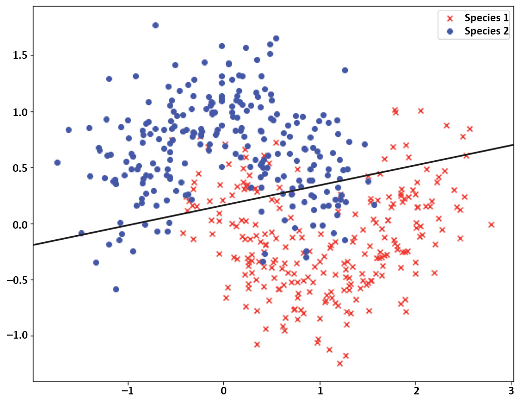
Figure 3.14: Underfitting
If we increase the flexibility of the neural network by adding more layers to it and increase the number of units in each layer, we can train a better model and succeed in capturing the non-linearity in the decision boundary. Such a model can be seen in the following plot. This is a model with a low training error rate and low-test error rate (again, the test error rate is slightly higher than the training error rate). Having a low training error rate and a slight difference between the test error rate and the training error rate is indicative of a model with low bias and low variance. A model with low bias and low variance represents the right amount of fitting for a given dataset:

Figure 3.15: Correct fit
But what will happen if we increase the flexibility of the neural network even more? By adding too much flexibility to the model, it will learn not only the patterns and relations in the training data but also the noise in them. In other words, the model will fit each individual training example as opposed to fitting only to the overall trends and relations in them. The following plot shows such a system. Evaluating this model will show a very low training error rate and a high-test error rate (with a large difference between the training error rate and test error rate). This is a model with low bias and high variance, and this situation is called overfitting:

Figure 3.16: Overfitting
Evaluating the model on both the training set and the test set and comparing their error rates provide valuable information on whether the current model is right for a given dataset. Also, in cases where the current model is not fitting the dataset correctly, it is possible to determine whether it is overfitting or underfitting to the data and change the model accordingly to find the right model. For example, if the model is underfitting, you can make the network larger. On the other hand, if the model is overfitting, you can reduce the overfitting by making the network smaller or providing more training data to it. There are many methods that can be implemented to prevent underfitting or overfitting in practice, one of which we will explore in the next section.
Early Stopping
Sometimes, the flexibility of a model is right for the dataset but overfitting or underfitting is still happening. This is because we are training the model for either too many iterations or too few iterations. When using an iterative optimizer such as gradient descent, the optimizer tries to fit the training data better and better in every iteration. Therefore, if we keep updating the parameters after the patterns in the data are learned, it will start fitting to the individual data examples.
By observing the training and test error rates in every iteration, it is possible to determine when the network is starting to overfit to the training data and stop the training process before this happens. Regions associated with underfitting and overfitting have been labeled on the following plot. The correct number of iterations for training the model can be determined from the region at which the test error rate has its lowest value. We labeled this region as the right fit on the plot and it can be seen that, in this region, both the training error rate and the test error rate are low:

Figure 3.17: Plot of training error rate and test error rate while training a model
You can easily store the values for training loss and test loss in every epoch while training with Keras. To do this, you need to provide the test set as the validation_data argument when defining the fit() method for the model and store it in a history dictionary:
history = model.fit(X_train, y_train, validation_data=(X_test, y_test))
You can plot the values stored in history later to find the correct number of iterations to train your model with:
import matplotlib.pyplot as plt
import matplotlib
# plot training loss
plt.plot(history.history['loss'])
# plot test loss
plt.plot(history.history['val_loss'])
In general, since deep neural networks are highly flexible models, the chance of overfitting happening is very high. There is a whole group of techniques, called regularization techniques, that have been developed to reduce overfitting in machine learning models in general, and deep neural networks in particular. You will learn more about these techniques in Chapter 5, Improving Model Accuracy. In the next activity, we will put our understanding into practice and attempt to find the optimal number of epochs to train for so as to prevent overfitting.
Activity 3.02: Advanced Fibrosis Diagnosis with Neural Networks
In this activity, you are going to use a real dataset to predict whether a patient has advanced fibrosis based on measurements such as age, gender, and BMI. The dataset consists of information for 1,385 patients who underwent treatment dosages for hepatitis C. For each patient, 28 different attributes are available, as well as a class label, which can only take two values: 1, indicating advanced fibrosis, and 0, indicating no indication of advanced fibrosis. This is a binary/two-class classification problem with an input dimension equal to 28.
In this activity, you will implement different deep neural network architectures to perform this classification. Plot the trends in the training error rates and test error rates and determine how many epochs the final classifier needs to be trained for:
Note
The dataset that's being used in this activity can be found here: https://packt.live/39pOUMT.

Figure 3.18: Schematic view of the binary classifier for a diabetes diagnosis
Follow these steps to complete this activity:
- Import all the necessary dependencies. Load the dataset from the data subfolder of the Chapter03 folder from GitHub:
X = pd.read_csv('../data/HCV_feats.csv')
y = pd.read_csv('../data/HCV_target.csv')
- Print the number of examples in the dataset, the number of features available, and the possible values for the class labels.
- Scale the data using the StandardScalar function from sklearn.preprocessing and split the dataset into the training set and test set with an 80:20 ratio. Then, print the number of examples in each set after splitting.
- Implement a shallow neural network with one hidden layer of size 3 and a tanh activation function to perform the classification. Compile the model with the following values for the hyperparameters: optimizer = 'sgd', loss = 'binary_crossentropy', metrics = ['accuracy']
- Fit the model with the following hyperparameters and store the values for training error rate and test error rate during the training process: batch_size = 20, epochs = 100, validation_split=0.1, and shuffle=False.
- Plot the training error rate and test error rate for every epoch of training. Use the plot to determine at which epoch the network is starting to overfit to the dataset. Also, print the values of the best accuracy that were reached on the training set and on the test set, as well as the loss and accuracy that were evaluated on the test dataset.
- Repeat steps 4 and 5 for a deep neural network with two hidden layers (the first layer of size 4 and the second layer of size 3) and a 'tanh' activation function for both layers in order to perform the classification.
Note
The solution for this activity can be found on page 374.
Please note that both models were able to achieve better accuracy on the training or validation set compared to the test set, and the training error rate kept decreasing when it was trained for a significant number of epochs. However, the validation error rate decreased during training to a certain value, and after that, it started increasing, which is indicative of overfitting to the training data. The maximum validation accuracy corresponds to the point on the plots where the validation loss is at its lowest and is truly representative of how well the model will perform on independent examples later.
It can be seen from the results that the model with one hidden layer is able to reach a lower validation and test error rate in comparison to the two-layer models. From this, we may conclude that this model is the best match for this particular problem. The model with one hidden layer shows a large amount of bias, indicated by the large gap between the training and validation errors, and both were still decreasing, indicating that the model can be trained for more epochs. Lastly, it can be determined from the plots that we should stop training around the region where the validation error rate starts increasing to prevent the model from overfitting to the data points.
Summary
In this chapter, you extended your knowledge of deep learning, from understanding the common representations and terminology to implementing them in practice through exercises and activities. You learned how forward propagation in neural networks works and how it is used for predicting outputs, how the loss function works as a measure of model performance, and how backpropagation is used to compute the derivatives of loss functions with respect to model parameters.
You also learned about gradient descent, which uses the gradients that are computed by backpropagation to gradually update the model parameters. In addition to basic theory and concepts, you implemented and trained both shallow and deep neural networks with Keras and utilized them to make predictions about the output of a given input.
To evaluate your models appropriately, you split a dataset into a training set and a test set as an alternative approach to improving network evaluation and learned the reasons why evaluating a model on training examples can be misleading. This helped further your understanding of overfitting and underfitting that can happen when training a model. Finally, you utilized the training error rate and test error rate to detect overfitting and underfitting in a network and implemented early stopping in order to reduce overfitting in a network.
In the next chapter, you will learn about the Keras wrapper with scikit-learn and how to use it to further improve model evaluation by using resampling methods such as cross-validation. By doing this, you will learn how to find the best set of hyperparameters for a deep neural network.