Overview
This chapter introduces you to building Keras wrappers with scikit-learn. You will learn to apply cross-validation to evaluate deep learning models, and create user-defined functions to implement deep learning models along with cross-validation. By the end of this chapter, you will be able to build robust models that perform as well on new, unseen data as they do on the trained data.
Introduction
In the previous chapter, we experimented with different neural network architectures. We were able to evaluate the performance of the different models by observing the loss and accuracy during the course of the training process. This helped us determine when the model was underfitting or overfitting the training data and how to use techniques such as early stopping to prevent overfitting.
In this chapter, you will learn about cross-validation. This is a resampling technique that leads to a very accurate and robust estimation of a model's performance, in comparison to the model evaluation approaches we discussed in the previous chapters.
This chapter starts with an in-depth discussion about why we need to use cross-validation for model evaluation, the underlying basics of cross-validation, its variations, and a comparison between them. Next, we will implement cross-validation on Keras deep learning models. We will also use Keras wrappers with scikit-learn to allow Keras models to be treated as estimators in a scikit-learn workflow. You will then learn how to implement cross-validation in scikit-learn and finally bring it all together and perform cross-validation using scikit-learn on Keras deep learning models.
Lastly, you will learn about how to use cross-validation to perform more than just model evaluation, and how a cross-validation estimation of model performance can be used to compare different models and select the one that results in the best performance on a particular dataset. You will also use cross-validation to improve the performance of a given model by finding the best set of hyperparameters for it. We will implement the concepts that we will learn about in this chapter in three activities, each involving a real-life dataset.
Cross-Validation
Resampling techniques are an important group of techniques in statistical data analysis. They involve repeatedly drawing samples from a dataset to create the training set and the test set. At each repetition, they fit and evaluate the model using the samples drawn from the dataset for the training set and the test set at that repetition.
Using these techniques can provide us with information about the model that is otherwise not obtainable by fitting and evaluating the model only once, using one training set and one test set. Since resampling methods involve fitting a model to the training data several times, they are computationally expensive. Therefore, when it comes to deep learning, we only implement them in the cases where the dataset and the network are relatively small, and the available computational power allows us to do so.
In this section, you will learn about a very important resampling method called cross-validation. Cross-validation is one of the most important and most commonly used resampling methods. It computes the best estimation of model performance on new, unseen examples when given a limited dataset. We will also explore the basics of cross-validation, its two variations, and a comparison between them.
Drawbacks of Splitting a Dataset Only Once
In the previous chapter, we mentioned that evaluating a model on the same dataset that's used to train the model is a methodological mistake. Since the model has been trained to reduce the error on this particular set of examples, its performance on it is highly biased. That is why the error rate on training data is always an underestimation of the error rate on new examples. We learned that one way to solve this problem is to randomly hold out a subset of the data as a test set for evaluation and fit the model on the rest of the data, which is called the training set. An illustration of this approach can be seen in the following image:

Figure 4.1: Overview of training set/test set split
As we mentioned previously, assigning the data to either the training set or the test set is completely random. This means that if we repeat this process, different data will be assigned to the test set and training set each time. The test error rate that's reported by this approach can vary a lot, depending on which examples are in the test set and which examples are in the training set.
Example
Let's look at an example. Here, we have built a single-layer neural network for the hepatitis C dataset that you saw in Activity 3.02, Advanced Fibrosis Diagnosis with Neural Networks in Chapter 3, Deep Learning with Keras. We used the training set/test set approach to compute the test error associated with this model. Instead of splitting and training only once, if we split the data into five separate datasets and repeated this process five times, we might expect five different plots for the test error rates. The test error rates for each of these five experiments can be seen in the following plot:

Figure 4.2: Plot of test error rates with five different training set/test set splits on an example dataset
As you can see, the test error rate is quite different in each experiment. This variation in the models' evaluation results indicates that the simple strategy of splitting the dataset into a training set and a test set only once may not lead to a robust and accurate estimation of the model's performance.
To summarize, the training set/test set approach that we learned about in the previous chapter has the obvious advantage of being simple, easy to implement, and computationally inexpensive. However, it has drawbacks too, which are as follows:
- The first drawback is that its estimation of the model's error rate strongly depends on exactly which data is assigned to the test set and which data is assigned to the training set.
- The second drawback is that, in this approach, we are only training the model on a subset of the data. Machine learning models tend to perform worse when they are trained using a small amount of data.
Since the performance of a model can be improved by training it on the entire dataset, we are always looking for ways to include all the available data points in training. Additionally, we are interested in finding a robust estimation of the model's performance by including all the available data points in the evaluation. These objectives can be accomplished with the use of cross-validation techniques. The following are the two methods of cross-validation:
- K-fold cross-validation
- Leave-one-out cross-validation
K-Fold Cross-Validation
In k-fold cross-validation, instead of dividing the dataset into two subsets, we divide the dataset into k approximately equal-sized subsets or folds. In the first iteration of the method, the first fold is considered a test set. The model is trained on the remaining k-1 folds, and then it is evaluated on the first fold (the first fold is used to estimate the test error rate).
This process is repeated k times, and a different fold is used as the test set in each iteration, while the remaining folds are used as the training set. Eventually, the method results in k different test error rates. The final k-fold cross-validation estimate of the model's error rate is computed by averaging these k test error rates.
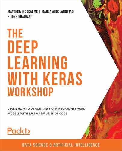
The following diagram illustrates the dataset splitting process in the k-fold cross-validation method:

Figure 4.3: Overview of dataset splitting in the k-fold cross-validation method
In practice, we usually perform k-fold cross-validation with k=5 or k=10, and these are the recommended values if you are struggling to select a value for your dataset. Deciding on the number of folds to use is dependent on the number of examples in the dataset and the available computational power. If k=5, the model will be trained and evaluated five times, while if k=10, this process will be repeated 10 times. The higher the number of folds, the longer it will take to perform k-fold cross-validation.
In k-fold cross-validation, the assignment of examples to each fold is completely random. However, by looking at the preceding diagram, you will see that, in the end, every single piece of data is used for both training and evaluation. That's why if you repeat k-fold cross-validation many times on the same dataset and the same model, the final reported test error rates will be almost identical. Therefore, k-fold cross-validation does not suffer from high variance in its results, in contrast to the training set/test set approach. Now, we will take a look at the second form of cross-validation: leave-one-out validation.
Leave-One-Out Cross-Validation
Leave-One-Out (LOO) is a variation of the cross-validation technique in which, instead of dividing the dataset into two comparable-sized subsets for the training set and test set, only one single piece of data is used for evaluation. If there are n data examples in the entire dataset, at each iteration of LOO cross-validation, the model is trained on n-1 examples and the single remaining example is used to compute the test error rate.
Using only one example for estimating the test error rate leads to an unbiased but high variance estimation of model performance; it is unbiased because this one example has not been used in training the model, it has high variance because it is computed based on only one data example, and it will vary depending on which exact data example is used. This process is repeated n times, and, at each iteration, a different data example is used for evaluation. In the end, the method will result in n different test error rates, and the final LOO cross-validation test error estimation is computed by averaging these n error rates.
An illustration of the dataset splitting process in the LOO cross-validation method can be seen in the following diagram:
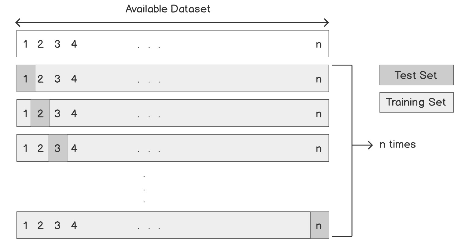
Figure 4.4: Overview of dataset splitting in the LOO cross-validation method
In each iteration of LOO cross-validation, almost all the examples in the dataset are used to train the model. On the other hand, in the training set/test set approach, a relatively large subset of data is used for evaluation and not used in training. Therefore, the LOO estimation of model performance is much closer to the performance of a model that is trained on the entire dataset, and this is the main advantage of LOO cross-validation over the training set/test set approach.
Additionally, since in each iteration of LOO cross-validation only one unique data example is used for evaluation, and every single data example is used for training as well, there is no randomness associated with this method. Therefore, if you repeat LOO cross-validation many times on the same dataset and the same model, the final reported test error rates will be exactly the same each time.
The drawback of LOO cross-validation is that it is computationally expensive. The reason for this is that the model needs to be trained n times, and in cases where n is large and/or the network is large, it will take a long time to complete. Both LOO and k-fold cross-validation have their advantages and disadvantages, all of which we will compare in the next section.
Comparing the K-Fold and LOO Methods
By comparing the two preceding diagrams, it is obvious that LOO cross-validation is, in fact, a special case of k-fold cross-validation, where k=n. However, as was mentioned previously, choosing k=n is computationally very expensive in comparison to choosing k=5 or k=10.
Therefore, the first advantage of k-fold cross-validation over LOO cross-validation is that it is computationally less expensive. The following table compares the k-fold with low-k, k-fold with high-k and LOO, and no cross-validation with respect to bias and variance. The table shows that the highest bias comes with a simple train-test split approach and that the highest variance comes with leave-one-put cross-validation. In the middle is k-fold cross-validation. This is why k-fold cross-validation is generally the most appropriate choice for most machine learning tasks:
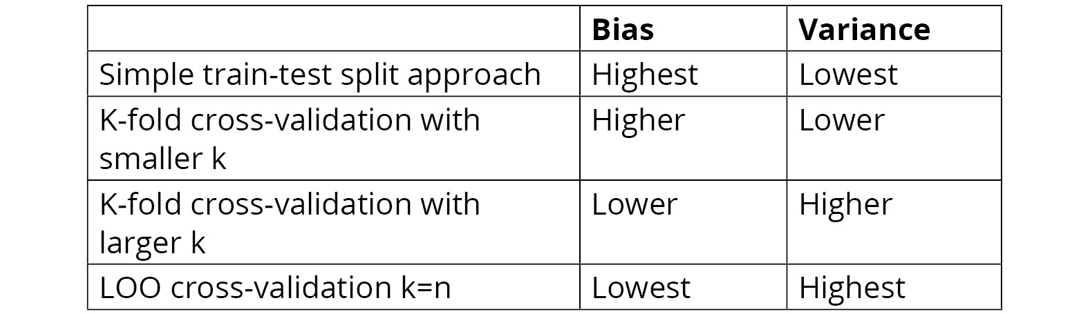
Figure 4.5: Comparing the train-test split, k-fold cross-validation, and LOO cross-validation methods
The following plot compares the training set/test set approach, k-fold cross-validation, and LOO cross-validation in terms of bias and variance:

Figure 4.6: Comparing the training set/test set approach, k-fold cross-validation, and LOO cross-validation in terms of bias and variance
Generally, in machine learning and data analysis, the most desirable model is the one with the lowest bias and the lowest variance. As shown in the preceding plot, the region labeled in the middle of the graph, where both bias and variance are low, is of interest. It turns out that this region is equivalent to k-fold cross-validation with k between 5 and 10. In the next section, we will explore how to implement various methods of cross-validation in practice.
Cross-Validation for Deep Learning Models
In this section, you will learn about using the Keras wrapper with scikit-learn, which is a helpful tool that allows us to use Keras models as part of a scikit-learn workflow. As a result, scikit-learn methods and functions, such as the one for performing cross-validation, can easily be applied to Keras models.
You will learn, step-by-step, how to implement what you learned about cross-validation in the previous section using scikit-learn. Furthermore, you will learn how to use cross-validation to evaluate Keras deep learning models using the Keras wrapper with scikit-learn. Lastly, you will practice what you have learned by solving a problem involving a real dataset.
Keras Wrapper with scikit-learn
When it comes to general machine learning and data analysis, the scikit-learn library is much richer and easier to use than Keras. That is why being able to use scikit-learn methods on Keras models will be of great value.
Fortunately, Keras comes with a helpful wrapper, keras.wrappers.scikit_learn, that allows us to build scikit-learn interfaces for deep learning models that can be used as classification or regression estimators in scikit-learn. There are two types of wrapper: one for classification estimators and one for regression estimators. The following code is used to define these scikit-learn interfaces:
keras.wrappers.scikit_learn.KerasClassifier(build_fn=None, **sk_params)
# wrappers for classification estimators
keras.wrappers.scikit_learn.KerasRegressor(build_fn=None, **sk_params)
# wrappers for regression estimators
The build_fn argument needs to be a callable function where a Keras sequential model is defined, compiled and returned inside its body.
The sk_params argument can take parameters for building the model (such as activation functions for layers) and parameters for fitting the model (such as the number of epochs and batch size). This will be put into practice in the following exercise, where we will use Keras wrappers for a regression problem.
Note
All the activities in this chapter will be developed in a Jupyter notebook. Please download this book's GitHub repository, along with all the prepared templates, which can be found here:
Exercise 4.01: Building the Keras Wrapper with scikit-learn for a Regression Problem
In this exercise, you will learn the step-by-step process of building the wrapper for a Keras deep learning model so that it can be used in a scikit-learn workflow. First, load in the dataset of 908 data points of a regression problem, where each record describes six attributes of a chemical, and the target is the acute toxicity toward the fish Pimephales promelas, or LC50:
Note
Watch out for the slashes in the string below. Remember that the backslashes ( ) are used to split the code across multiple lines, while the forward slashes ( / ) are part of the path.
# import data
import pandas as pd
colnames = ['CIC0', 'SM1_Dz(Z)', 'GATS1i',
'NdsCH', 'NdssC','MLOGP', 'LC50']
data = pd.read_csv('../data/qsar_fish_toxicity.csv',
sep=';', names=colnames)
X = data.drop('LC50', axis=1)
y = data['LC50']
# Print the sizes of the dataset
print("Number of Examples in the Dataset = ", X.shape[0])
print("Number of Features for each example = ", X.shape[1])
# print output range
print("Output Range = [%f, %f]" %(min(y), max(y)))
This is the expected output:
Number of Examples in the Dataset = 908
Number of Features for each example = 6
Output Range = [0.053000, 9.612000]
Since the output in this dataset takes a numerical value, this is a regression problem. The goal is to build a model that predicts the acute toxicity toward the fish LC50, given the other attributes of the chemical. Now, let's go through the steps:
- Define a function that builds and returns a Keras model for this regression problem. The Keras model that you define must have a single hidden layer of size 8 with ReLU activation functions. Also, use the Mean Squared Error (MSE) loss function and the Adam optimizer to compile the model:
from keras.models import Sequential
from keras.layers import Dense, Activation
# Create the function that returns the keras model
def build_model():
# build the Keras model
model = Sequential()
model.add(Dense(8, input_dim=X.shape[1],
activation='relu'))
model.add(Dense(1))
# Compile the model
model.compile(loss='mean_squared_error',
optimizer='adam')
# return the model
return model
- Now, use the Keras wrapper with scikit-learn to create the scikit-learn interface for your model. Remember that you need to provide the epochs, batch_size, and verbose arguments here:
# build the scikit-Learn interface for the keras model
from keras.wrappers.scikit_learn import KerasRegressor
YourModel = KerasRegressor(build_fn= build_model,
epochs=100,
batch_size=20,
verbose=1)
Now, YourModel is ready to be used as a regression estimator in scikit-learn.
In this exercise, we learned how to build a Keras wrapper with scikit-learn for a regression problem by using a simulated dataset.
Note
To access the source code for this specific section, please refer to https://packt.live/38nuqVP.
You can also run this example online at https://packt.live/31MLgMF.
We will continue implementing cross-validation using this dataset in the rest of the exercises in this chapter.
Cross-Validation with scikit-learn
In the previous chapter, you learned that you can perform training set/test set splitting easily in scikit-learn. Let's assume that your original dataset is stored in X and y arrays. You can split them randomly into a training set and a test set using the following commands:
from sklearn.model_selection import train_test_split
X_train, X_test, y_train, y_test = train_test_split
(X, y, test_size=0.3,
random_state=0)
The test_size argument can be assigned to any number between 0 and 1, depending on how large you would like the test set to be. By providing an int number for a random_state argument, you will be able to select the seed for the random number generator.
The easiest way to perform cross-validation in scikit-learn is by using the cross_val_score function. In order to do this, you need to define your estimator first (in our case, the estimator will be a Keras model). Then, you will be able to perform cross-validation on your estimator/model using the following commands:
from sklearn.model_selection import cross_val_score
scores = cross_val_score(YourModel, X, y, cv=5)
Notice that we provide the Keras model and the original dataset as arguments to the cross_val_score function, along with the number of folds (the cv argument). Here, we used cv=5, so the cross_val_score function will randomly split the dataset into five-folds and perform training and fitting on the model five times using five different training and test sets. It will compute the default metric for model evaluation (or the metrics given to the Keras model when defining it) at each iteration/fold and store them in scores. We can print the final cross-validation score as follows:
print(scores.mean())
Earlier, we mentioned that the score that's returned by the cross_val_score function is the default metric for our model or the metric that we determined for it when defining our model. However, it is possible to change the cross-validation metric by providing the desired metric as a scoring argument when calling the cross_val_score function.
Note
You can learn more about how to provide the desired metric in the scoring argument of the cross_val_score function here: https://scikit-learn.org/stable/modules/model_evaluation.html#scoring-parameter.
By providing an integer number for the cv argument of the cross_val_score function, we are telling the function to perform k-fold cross-validation on the dataset. However, there are several other iterators available in scikit-learn that we can assign to cv to perform other variations of cross-validation on the dataset. For example, the following code block will perform LOO cross-validation on the dataset:
from sklearn.model_selection import LeaveOneOut
loo = LeaveOneOut()
scores = cross_val_score(YourModel, X, y, cv=loo)
In the next section, we will explore k-fold cross-validation in scikit-learn and see how it can be used with Keras models.
Cross-Validation Iterators in scikit-learn
A list of the most commonly used cross-validation iterators available in scikit-learn is provided here, along with a brief description of each of them:
- KFold(n_splits=?)
This divides the dataset into k folds or groups. The n_splits argument is required to determine how many folds to use. If n_splits=n, it will be equivalent to LOO cross-validation.
- RepeatedKFold(n_splits=?, n_repeats=?, random_state=random_state)
This will repeat k-fold cross-validation n_repeats times.
- LeaveOneOut()
This will split the dataset for LOO cross-validation.
- ShuffleSplit(n_splits=?, test_size=?, random_state= random_state)
This will generate an n_splits number of random and independent training set/test set dataset splits. It is possible to store the seed for the random number generator using the random_state argument; if you do this, the dataset splits will be reproducible.
In addition to the regular iterators, such as the ones mentioned here, there are stratified versions as well. Stratified sampling is useful when the number of examples in different classes of a dataset is unbalanced. For example, imagine that we want to design a classifier to predict whether someone will default on their credit card debt, where almost 95% of the examples in the dataset are in the negative class. Stratified sampling makes sure that the relative class frequencies are preserved in each training set/test set split. It is recommended to use the stratified versions of iterators for such cases.
Usually, before using a training set to train and evaluate a model, we perform preprocessing on it to scale the examples so that they have a mean equal to 0 and a standard deviation equal to 1. In the training set/test set approach, we need to scale the training set and store the transformation. The following code block will do this for us:
from sklearn.preprocessing import StandardScaler
scaler = StandardScaler()
X_train = scaler.fit_transform(X_train)
X_test = scaler.transform(X_test)
Here's an example of performing stratified k-fold cross-validation with k=5 on our X, y dataset:
from sklearn.model_selection import StratifiedKFold
skf = StratifiedKFold(n_splits=5)
scores = cross_val_score(YourModel, X, y, cv=skf)
Note
You can learn more about cross-validation iterators in scikit-learn here:
https://scikit-learn.org/stable/modules/cross_validation.html#cross-validation-iterators.
Now that we understand cross-validation iterators, we can put them into practice in an exercise.
Exercise 4.02: Evaluating Deep Neural Networks with Cross-Validation
In this exercise, we will bring all the concepts and methods that we have learned about in this topic about cross-validation together. We will go through all the steps one more time, from defining a Keras deep learning model to transferring it to a scikit-learn workflow and performing cross-validation in order to evaluate its performance. In a sense, this exercise is a recap of what we have learned so far, and what is covered here will be extremely helpful for Activity 4.01, Model Evaluation Using Cross-Validation for an Advanced Fibrosis Diagnosis Classifier:
- The first step is always to load the dataset that you would like to build the model for. First, load in the dataset of 908 data points of a regression problem, where each record describes six attributes of a chemical and the target is the acute toxicity toward the fish Pimephales promelas, or LC50:
# import data
import pandas as pd
colnames = ['CIC0', 'SM1_Dz(Z)', 'GATS1i',
'NdsCH', 'NdssC','MLOGP', 'LC50']
data = pd.read_csv('../data/qsar_fish_toxicity.csv',
sep=';', names=colnames)
X = data.drop('LC50', axis=1)
y = data['LC50']
# Print the sizes of the dataset
print("Number of Examples in the Dataset = ", X.shape[0])
print("Number of Features for each example = ", X.shape[1])
# print output range
print("Output Range = [%f, %f]" %(min(y), max(y)))
The output is as follows:
Number of Examples in the Dataset = 908
Number of Features for each example = 6
Output Range = [0.053000, 9.612000]
- Define the function that returns the Keras model with a single hidden layer of size 8 with ReLU activation functions using the Mean Squared Error (MSE) loss function and the Adam optimizer:
from keras.models import Sequential
from keras.layers import Dense, Activation
# Create the function that returns the keras model
def build_model():
# build the Keras model
model = Sequential()
model.add(Dense(8, input_dim=X.shape[1],
activation='relu'))
model.add(Dense(1))
# Compile the model
model.compile(loss='mean_squared_error',
optimizer='adam')
# return the model
return model
- Set the seed and use the wrapper to build the scikit-learn interface for the Keras model we defined in the function in step 2:
# build the scikit-Learn interface for the keras model
from keras.wrappers.scikit_learn import KerasRegressor
import numpy as np
from tensorflow import random
seed = 1
np.random.seed(seed)
random.set_seed(seed)
YourModel = KerasRegressor(build_fn= build_model,
epochs=100, batch_size=20,
verbose=1 , shuffle=False)
- Define the iterator to use for cross-validation. Let's perform 5-fold cross-validation:
# define the iterator to perform 5-fold cross-validation
from sklearn.model_selection import KFold
kf = KFold(n_splits=5)
- Call the cross_val_score function to perform cross-validation. This step will take a while to complete, depending on the computational power that's available:
# perform cross-validation on X, y
from sklearn.model_selection import cross_val_score
results = cross_val_score(YourModel, X, y, cv=kf)
- Once cross-validation has been completed, print the final cross-validation estimation of model performance (the default metric for performance will be the test loss):
# print the result
print(f"Final Cross-Validation Loss = {abs(results.mean()):.4f}")
Here's an example output:
Final Cross-Validation Loss = 0.9680
The cross-validation loss states that the Keras model that was trained on this dataset is able to predict the LC50 of the chemicals with an average loss of 0.9680. We will try to examine this model further in the next exercise.
These were all the steps that are required in order to evaluate a Keras deep learning model using cross-validation in scikit-learn. Now, we will put them into practice in an activity.
Note
To access the source code for this specific section, please refer to https://packt.live/3eRTlTM.
You can also run this example online at https://packt.live/31IdVT0.
Activity 4.01: Model Evaluation Using Cross-Validation for an Advanced Fibrosis Diagnosis Classifier
We learned about the hepatitis C dataset in Activity 3.02, Advanced Fibrosis Diagnosis with Neural Networks of Chapter 3, Deep Learning with Keras. The dataset consists of information for 1385 patients who underwent treatment dosages for hepatitis C. For each patient, 28 different attributes are available, such as age, gender, and BMI, as well as a class label, which can only take two values: 1, indicating advanced fibrosis, and 0, indicating no indication of advanced fibrosis. This is a binary/two-class classification problem with an input dimension equal to 28.
In Chapter 3, Deep Learning with Keras, we built Keras models to perform classification on this dataset. We trained and evaluated the models using training set/test set splitting and reported the test error rate. In this activity, we are going to use what we learned in this topic to train and evaluate a deep learning model using k-fold cross-validation. We will use the model that resulted in the best test error rate from the previous activity. The goal is to compare the cross-validation error rate with the training set/test set approach error rate:
- Import the necessary libraries. Load the dataset from the data subfolder of the Chapter04 folder from GitHub using X = pd.read_csv('../data/HCV_feats.csv'), y = pd.read_csv('../data/HCV_target.csv'). Print the number of examples in the dataset, the number of features available, and the possible values for the class labels.
- Define the function that returns the Keras model. The Keras model will be a deep neural network with two hidden layers, where the first hidden layer is of size 4 and the second hidden layer is of size 2, and use the tanh activation function to perform the classification. Use the following values for the hyperparameters:
optimizer = 'adam', loss = 'binary_crossentropy', metrics = ['accuracy']
- Build the scikit-learn interface for the Keras model with epochs=100, batch_size=20, and shuffle=False. Define the cross-validation iterator as StratifiedKFold with k=5. Perform k-fold cross-validation on the model and store the scores.
- Print the accuracy for each iteration/fold, plus the overall cross-validation accuracy and its associated standard deviation.
- Compare this result with the result from Activity 3.02, Advanced Fibrosis Diagnosis with Neural Networks of Chapter 3, Deep Learning with Keras.
After implementing the preceding steps, the expected output will look as follows:
Test accuracy at fold 1 = 0.5198556184768677
Test accuracy at fold 2 = 0.4693140685558319
Test accuracy at fold 3 = 0.512635350227356
Test accuracy at fold 4 = 0.5740072131156921
Test accuracy at fold 5 = 0.5523465871810913
Final Cross Validation Test Accuracy: 0.5256317675113678
Standard Deviation of Final Test Accuracy: 0.03584760640500936
Note
The solution for this activity can be found on page 381.
The accuracy we received from training set/test set approach we performed in Activity 3.02, Advanced Fibrosis Diagnosis with Neural Networks of Chapter 3, Deep Learning with Keras, was 49.819%, which is lower than the test accuracy we achieved when performing 5-fold cross-validation on the same deep learning model and the same dataset, but lower than the accuracy on one of the folds.
The reason for this difference is that the test error rate resulting from the training set/test set approach was computed by only including a subset of the data points in the model's evaluation. On the other hand, the test error rate here is computed by including all the data points in the evaluation, and therefore this estimation of the model's performance is more accurate and more robust, performing better on the unseen test dataset.
In this activity, we used cross-validation to perform a model evaluation on a problem involving a real dataset. Improving model evaluation is not the only purpose of using cross-validation, and it can be used to select the best model or parameters for a given problem as well.
Model Selection with Cross-Validation
Cross-validation provides us with robust estimation of model performance on unseen examples. For this reason, it can be used to decide between two models for a particular problem or to decide which model parameters (or hyperparameters) to use for a particular problem. In these cases, we would like to find out which model or which set of model parameters/hyperparameters results in the lowest test error rate. Therefore, we will select that model or that set of parameters/hyperparameters for our problem.
In this section, you are going to practice using cross-validation for this purpose. You will learn how to define a set of hyperparameters for your deep learning model and then write user-defined functions in order to perform cross-validation on your model for each of the possible combinations of hyperparameters. Then, you will observe which combination of hyperparameters leads to the lowest test error rate, and that combination will be your choice for your final model.
Cross-Validation for Model Evaluation versus Model Selection
In this section, we are going to go deeper into what it means to use cross-validation for model evaluation versus model selection. So far, we have learned that evaluating a model on the training set results in an underestimation of the model's error rate on unseen examples. Splitting the dataset into a training set and a test set gives us a more accurate estimation of the model's performance but suffers from high variance.
Lastly, cross-validation results in a much more robust and accurate estimation of the model's performance on unseen examples. An illustration of the error rate estimations resulting from these three approaches for model evaluation can be seen in the following plot.
The following plot shows the case where the error rate estimation in the training set/test set approach is slightly lower than the cross-validation estimation. However, it is important to remember that the training set/test set error rate can be higher than the cross-validation estimation error rate as well, depending on what data is included in the test set (hence the high variance problem). On the other hand, the error rate resulting from performing an evaluation on the training set is always lower than the other two approaches:
Figure 4.7: Illustration of the error rate estimations resulting from the three approaches to model evaluation
We have established that cross-validation leads to the best estimation of a model's performance on independent data examples. Knowing this, we can use cross-validation to decide which model to use for a particular problem. For example, if we have four different models and we would like to decide which one is a better fit for a particular dataset, we can train and evaluate each of the four models using cross-validation and choose the model with the lowest cross-validation error rate as our final model for the dataset. The following plot shows the cross-validation error rate associated with four hypothetical models. From this, we can conclude that Model 1 is the best fit for the problem, while Model 4 is the worst choice. These four models could be deep neural networks with a different number of hidden layers and a different number of units in their hidden layers:

Figure 4.8: Illustration of cross-validation error rates associated with four hypothetical models
After we have found out which model is the best fit for a particular problem, the next step is choosing the best set of parameters or hyperparameters for that model. Previously, we discussed that when building a deep neural network, several hyperparameters need to be selected for the model, and several choices are available for each of these hyperparameters.
These hyperparameters include the type of activation function, loss function, and optimizer, plus the number of epochs and batch size. We can define the set of possible choices for each of these hyperparameters and then implement the model, along with cross-validation, to find the best combination of hyperparameters.
An illustration of the cross-validation error rates associated with four different sets of hyperparameters for a hypothetical deep learning model is shown in the following plot. From this, we can conclude that Set 1 is the best choice for this model since the line corresponding to Hyperparameters Set 1 has the lowest value for the cross-validation error rate:

Figure 4.9: Illustration of cross-validation error rates associated with four different sets of hyperparameters for a hypothetical deep learning model
In the next exercise, we will learn how to iterate through different model architectures and hyperparameters to find the set that results in an optimal model.
Exercise 4.03: Writing User-Defined Functions to Implement Deep Learning Models with Cross-Validation
In this exercise, you will learn how to use cross-validation for the purpose of model selection.
First, load in the dataset of 908 data points of a regression problem, where each record describes six attributes of a chemical and the target is the acute toxicity toward the fish Pimephales promelas, or LC50. The goal is to build a model to predict the LC50 of each chemical, given the chemical attributes:
# import data
import pandas as pd
import numpy as np
from tensorflow import random
colnames = ['CIC0', 'SM1_Dz(Z)', 'GATS1i', 'NdsCH',
'NdssC','MLOGP', 'LC50']
data = pd.read_csv('../data/qsar_fish_toxicity.csv',
sep=';', names=colnames)
X = data.drop('LC50', axis=1)
y = data['LC50']
Follow these steps to complete this exercise:
- Define three functions to return three Keras models. The first model should have one hidden layer of size 4, the second model should have one hidden layer of size 8, and the third model should have two hidden layers, with the first layer of size 4 and the second layer of size 2. Use a ReLU activation function for all the hidden layers. The goal is to find out which of these three models leads to the lowest cross-validation error rate:
# Define the Keras models
from keras.models import Sequential
from keras.layers import Dense
def build_model_1():
# build the Keras model_1
model = Sequential()
model.add(Dense(4, input_dim=X.shape[1],
activation='relu'))
model.add(Dense(1))
# Compile the model
model.compile(loss='mean_squared_error',
optimizer='adam')
# return the model
return model
def build_model_2():
# build the Keras model_2
model = Sequential()
model.add(Dense(8, input_dim=X.shape[1],
activation='relu'))
model.add(Dense(1))
# Compile the model
model.compile(loss='mean_squared_error',
optimizer='adam')
# return the model
return model
def build_model_3():
# build the Keras model_3
model = Sequential()
model.add(Dense(4, input_dim=X.shape[1],
activation='relu'))
model.add(Dense(2, activation='relu'))
model.add(Dense(1))
# Compile the model
model.compile(loss='mean_squared_error',
optimizer='adam')
# return the model
return model
- Write a loop to build the Keras wrapper and perform 3-fold cross-validation on the three models. Store the scores for each model:
"""
define a seed for random number generator so the result will be reproducible
"""
seed = 1
np.random.seed(seed)
random.set_seed(seed)
# perform cross-validation on each model
from keras.wrappers.scikit_learn import KerasRegressor
from sklearn.model_selection import KFold
from sklearn.model_selection import cross_val_score
results_1 = []
models = [build_model_1, build_model_2, build_model_3]
# loop over three models
for m in range(len(models)):
model = KerasRegressor(build_fn=models[m],
epochs=100, batch_size=20,
verbose=0, shuffle=False)
kf = KFold(n_splits=3)
result = cross_val_score(model, X, y, cv=kf)
results_1.append(result)
- Print the final cross-validation error rate for each of the models to find out which model has a lower error rate:
# print the cross-validation scores
print("Cross-Validation Loss for Model 1 =",
abs(results_1[0].mean()))
print("Cross-Validation Loss for Model 2 =",
abs(results_1[1].mean()))
print("Cross-Validation Loss for Model 3 =",
abs(results_1[2].mean()))
Here's an example output:
Cross-Validation Loss for Model 1 = 0.990475798256843
Cross-Validation Loss for Model 2 = 0.926532513151634
Cross-Validation Loss for Model 3 = 0.9735719371528117
Model 2 results in the lowest error rate, so we will use it in the steps that follow.
- Use cross-validation again to determine the number of epochs and batch size for the model that resulted in the lowest cross-validation error rate. Write the code that performs 3-fold cross-validation on every possible combination of epochs and batch-size in the ranges epochs=[100, 150] and batch_size=[20, 15] and store the scores:
"""
define a seed for random number generator so the result will be reproducible
"""
np.random.seed(seed)
random.set_seed(seed)
results_2 = []
epochs = [100, 150]
batches = [20, 15]
# Loop over pairs of epochs and batch_size
for e in range(len(epochs)):
for b in range(len(batches)):
model = KerasRegressor(build_fn= build_model_3,
epochs= epochs[e],
batch_size= batches[b],
verbose=0,
shuffle=False)
kf = KFold(n_splits=3)
result = cross_val_score(model, X, y, cv=kf)
results_2.append(result)
Note
The preceding code block uses two for loops to perform 3-fold cross-validation for all possible combinations of epochs and batch_size. Since there are two choices for each of them, four different pairs are possible and therefore cross-validation will be performed four times.
- Print the final cross-validation error rate for each of the epochs/batch_size pairs to find out which pair has the lowest error rate:
"""
Print cross-validation score for each possible pair of epochs, batch_size
"""
c = 0
for e in range(len(epochs)):
for b in range(len(batches)):
print("batch_size =", batches[b],",
epochs =", epochs[e], ", Test Loss =",
abs(results_2[c].mean()))
c += 1
Here's an example output:
batch_size = 20 , epochs = 100 , Test Loss = 0.9359159401008821
batch_size = 15 , epochs = 100 , Test Loss = 0.9642481369794683
batch_size = 20 , epochs = 150 , Test Loss = 0.9561188386646661
batch_size = 15 , epochs = 150 , Test Loss = 0.9359079093029896
As you can see, the performance for epochs=150 and batch_size=15, and for epochs=100 and batch_size=20, are almost the same. Therefore, we will choose epochs=100 and batch_size=20 in the next step to speed up this process.
- Use cross-validation again in order to decide on the activation function for the hidden layers and the optimizer for the model from activations = ['relu', 'tanh'] and optimizers = ['sgd', 'adam', 'rmsprop']. Remember to use the best pair of batch_size and epochs from the previous step:
# Modify build_model_2 function
def build_model_2(activation='relu', optimizer='adam'):
# build the Keras model_2
model = Sequential()
model.add(Dense(8, input_dim=X.shape[1],
activation=activation))
model.add(Dense(1))
# Compile the model
model.compile(loss='mean_squared_error',
optimizer=optimizer)
# return the model
return model
results_3 = []
activations = ['relu', 'tanh']
optimizers = ['sgd', 'adam', 'rmsprop']
"""
Define a seed for the random number generator so the result will be reproducible
"""
np.random.seed(seed)
random.set_seed(seed)
# Loop over pairs of activation and optimizer
for o in range(len(optimizers)):
for a in range(len(activations)):
optimizer = optimizers[o]
activation = activations[a]
model = KerasRegressor(build_fn= build_model_3,
epochs=100, batch_size=20,
verbose=0, shuffle=False)
kf = KFold(n_splits=3)
result = cross_val_score(model, X, y, cv=kf)
results_3.append(result)
Note
Notice that we had to modify the build_model_2 function by passing the activation, the optimizer, and their default values as arguments of the function.
- Print the final cross-validation error rate for each pair of activation and optimizer to find out which pair has the lower error rate:
"""
Print cross-validation score for each possible pair of optimizer, activation
"""
c = 0
for o in range(len(optimizers)):
for a in range(len(activations)):
print("activation = ", activations[a],",
optimizer = ", optimizers[o], ",
Test Loss = ", abs(results_3[c].mean()))
c += 1
Here's the output:
activation = relu , optimizer = sgd , Test Loss = 1.0123592540516995
activation = tanh , optimizer = sgd , Test Loss = 3.393908379781118
activation = relu , optimizer = adam , Test Loss = 0.9662686089392641
activation = tanh , optimizer = adam , Test Loss = 2.1369285960222144
activation = relu , optimizer = rmsprop , Test Loss = 2.1892826984214984
activation = tanh , optimizer = rmsprop , Test Loss = 2.2029884275363014
- The activation='relu' and optimizer='adam' pair results in the lowest error rate. Also, the result for the activation='relu' and optimizer='sgd' pair is almost as good. Therefore, we can use either of these optimizers in the final model to predict the aquatic toxicity for this dataset.
Note
To access the source code for this specific section, please refer to https://packt.live/2BYCwbg.
You can also run this example online at https://packt.live/3gofLfP.
Now, you are ready to practice model selection using cross-validation on another dataset. In Activity 4.02, Model Selection Using Cross-Validation for the Advanced Fibrosis Diagnosis Classifier, you will practice these steps further by implementing them by yourself on a classification problem with the hepatitis C dataset.
Note
Exercise 4.02, Evaluating Deep Neural Networks with Cross-Validation, and Exercise 4.03, Writing User-Defined Functions to Implement Deep Learning Models with Cross-Validation, involve performing k-fold cross-validation several times, so the steps may take several minutes to complete. If they are taking too long to complete, you may want to try speeding up the process by decreasing the number of folds or epochs or increasing the batch sizes. Obviously, if you do so, you will get different results compared to the expected outputs, but the same principles still apply for selecting the model and hyperparameters.
Activity 4.02: Model Selection Using Cross-Validation for the Advanced Fibrosis Diagnosis Classifier
In this activity, we are going to improve our classifier for the hepatitis C dataset by using cross-validation for model selection and hyperparameter selection. Follow these steps:
- Import the required packages. Load the dataset from the data subfolder of the Chapter04 folder from GitHub using X = pd.read_csv('../data/HCV_feats.csv'), y = pd.read_csv('../data/HCV_target.csv').
- Define three functions, each returning a different Keras model. The first Keras model will be a deep neural network with three hidden layers all of size 4 and ReLU activation functions. The second Keras model will be a deep neural network with two hidden layers, the first layer of size 4 and the second later of size 2, and ReLU activation functions. The third Keras model will be a deep neural network with two hidden layers, both of size 8, and a ReLU activation function. Use the following values for the hyperparameters:
optimizer = 'adam', loss = 'binary_crossentropy', metrics = ['accuracy']
- Write the code that will loop over the three models and perform 5-fold cross-validation on each of them (use epochs=100, batch_size=20, and shuffle=False in this step). Store all the cross-validation scores in a list and print the results. Which model results in the best accuracy?
Note
Steps 3, 4, and 5 of this activity involve performing 5-fold cross-validation three, four, and six times, respectively. Therefore, they may take some time to complete.
- Write the code that uses the epochs = [100, 200] and batches = [10, 20] values for epochs and batch_size. Perform 5-fold cross-validation for each possible pair on the Keras model that resulted in the best accuracy from step 3. Store all the cross-validation scores in a list and print the results. Which epochs and batch_size pair results in the best accuracy?
- Write the code that uses the optimizers = ['rmsprop', 'adam','sgd'] and activations = ['relu', 'tanh'] values for optimizer and activation. Perform 5-fold cross-validation for each possible pair on the Keras model that resulted in the best accuracy from step 3. Use the batch_size and epochs values that resulted in the best accuracy from step 4. Store all the cross-validation scores in a list and print the results. Which optimizer and activation pair results in the best accuracy?
Note
Please note that there is randomness associated with initializing weights and biases in a deep neural network, as well as with selecting which examples to include in each fold when performing k-fold cross-validation. Therefore, you might get a completely different result if you run the exact same code twice. For this reason, it is important to set up seeds when building and training neural networks, as well as when performing cross-validation. By doing this, you can make sure that you are repeating the exact same neural network initialization and the exact same training sets and test sets when you rerun the code.
After implementing these steps, the expected output will be as follows:
activation = relu , optimizer = rmsprop , Test accuracy = 0.5234657049179077
activation = tanh , optimizer = rmsprop , Test accuracy = 0.49602887630462644
activation = relu , optimizer = adam , Test accuracy = 0.5039711117744445
activation = tanh , optimizer = adam , Test accuracy = 0.4989169597625732
activation = relu , optimizer = sgd , Test accuracy = 0.48953068256378174
activation = tanh , optimizer = sgd , Test accuracy = 0.5191335678100586
Note
The solution for this activity can be found on page 384.
In this activity, you learned how to use cross-validation to evaluate deep neural networks in order to find the model that results in the lowest error rate for a classification problem. You also learned how to improve a given classification model by using cross-validation in order to find the best set of hyperparameters for it. In the next activity, we repeat this activity with a regression task.
Activity 4.03: Model Selection Using Cross-validation on a Traffic Volume Dataset
In this activity, you are going to practice model selection using cross-validation one more time. Here, we are going to use a simulated dataset that represents a target variable representing the volume of traffic in cars/hour across a city bridge and various normalized features related to traffic data such as the time of day and the traffic volume on the previous day. Our goal is to build a model that predicts the traffic volume across the city bridge given the various features.
The dataset contains 10000 records, and for each of them, 10 attributes/features are included. The goal is to build a deep neural network that receives the 10 features and predicts the traffic volume across the bridge. Since the output is a number, this is a regression problem. Let's get started:
- Import all the required packages.
- Print the input and output sizes to check the number of examples in the dataset and the number of features for each example. Also, you can print the range of the output (the output in this dataset represents the median value of owner-occupied homes in thousands of dollars).
- Define three functions, each returning a different Keras model. The first Keras model will be a shallow neural network with one hidden layer of size 10 and a ReLU activation function. The second Keras model will be a deep neural network with two hidden layers of size 10 and a ReLU activation function in each layer. The third Keras model will be a deep neural network with three hidden layers of size 10 and a ReLU activation function in each layer.
Use the following values as well:
optimizer = 'adam', loss = 'mean_squared_error'
Note
Steps 4, 5, and 6 of this activity involve performing 5-fold cross-validation three, four, and three times, respectively. Therefore, they may take some time to complete.
- Write the code to loop over the three models and perform 5-fold cross-validation on each of them (use epochs=100, batch_size=5, and shuffle=False in this step). Store all the cross-validation scores in a list and print the results. Which model results in the lowest test error rate?
- Write the code that uses the epochs = [80, 100] and batches = [5, 10] values for epochs and batch_size. Perform 5-fold cross-validation for each possible pair on the Keras model that resulted in the lowest test error rate from step 4. Store all the cross-validation scores in a list and print the results. Which epochs and batch_size pair results in the lowest test error rate?
- Write the code that uses optimizers = ['rmsprop', 'sgd', 'adam'] and perform 5-fold cross-validation for each possible optimizer on the Keras model that resulted in the lowest test error rate from step 4. Use the batch_size and epochs values that resulted in the lowest test error rate from step 5. Store all the cross-validation scores in a list and print the results. Which optimizer results in the lowest test error rate?
After implementing these steps, the expected output will be as follows:
optimizer= adam test error rate = 25.391812739372256
optimizer= sgd test error rate = 25.140230269432067
optimizer= rmsprop test error rate = 25.217947859764102
Note
The solution for this activity can be found on page 391.
In this activity, you learned how to use cross-validation to evaluate deep neural networks in order to find the model that results in the lowest error rate for a regression problem. Also, you learned how to improve a given regression model by using cross-validation in order to find the best set of hyperparameters for it.
Summary
In this chapter, you learned about cross-validation, which is one of the most important resampling methods. It results in the best estimation of model performance on independent data. This chapter covered the basics of cross-validation and its two different variations, leave-one-out and k-fold, along with a comparison of them.
Next, we covered the Keras wrapper with scikit-learn, which is a very helpful tool that allows scikit-learn methods and functions that perform cross-validation to be easily applied to Keras models. Following this, you were shown a step-by-step process of implementing cross-validation in order to evaluate Keras deep learning models using the Keras wrapper with scikit-learn.
Finally, you learned that cross-validation estimations of model performance can be used to decide between different models for a particular problem or to decide which parameters (or hyperparameters) should be used for a particular model. You practiced using cross-validation for this purpose by writing user-defined functions in order to perform cross-validation on different models or different possible combinations of hyperparameters and selecting the model or the set of hyperparameters that leads to the lowest test error rate for your final model.
In the next chapter, you will learn that what we did here in order to find the best set of hyperparameters for our model is, in fact, a technique called hyperparameter tuning or hyperparameter optimization. Also, you will learn how to perform hyperparameter tuning in scikit-learn by using a method called grid search and without the need to write user-defined functions to loop over possible combinations of hyperparameters.