
System Identification Based on Mutual Information Criteria
As a central concept in communication theory, mutual information measures the amount of information that one random variable contains about another. The larger the mutual information between two random variables is, the more information they share, and the better the estimation algorithm can be. Typically, there are two mutual information-based identification criteria: the minimum mutual information (MinMI) and the maximum mutual information (MaxMI) criteria. The MinMI criterion tries to minimize the mutual information between the identification error and the input signal such that the error signal contains as little as possible information about the input,1 while the MaxMI criterion aims to maximize the mutual information between the system output and the model output such that the model contains as much as possible information about the system in their outputs. Although the MinMI criterion is essentially equivalent to the minimum error entropy (MEE) criterion, their physical meanings are different. The MaxMI criterion is somewhat similar to the Infomax principle, an optimization principle for neural networks and other information processing systems. They are, however, different in their concepts. The Infomax states that a function that maps a set of input values I to a set of output values O should be chosen (or learned) so as to maximize the mutual information between I and O, subject to a set of specified constraints and/or noise processes. In the following, we first discuss the MinMI criterion.
6.1 System Identification Under the MinMI Criterion
The basic idea behind the MinMI criterion is that the model parameters should be determined such that the identification error contains as little as possible information about the input signal. The scheme of this identification method is shown in Figure 6.1. The objective function is the mutual information between the error and the input, and the optimal parameter is solved as
![]() (6.1)
(6.1)
where ![]() is the identification error at
is the identification error at ![]() time (the difference between the measurement
time (the difference between the measurement ![]() and the model output
and the model output ![]() ),
), ![]() is a vector consisting of all the inputs that have influence on the model output
is a vector consisting of all the inputs that have influence on the model output ![]() (possibly an infinite dimensional vector),
(possibly an infinite dimensional vector), ![]() is the set of all possible
is the set of all possible ![]() -dimensional parameter vectors.
-dimensional parameter vectors.

For a general causal system, ![]() will be
will be
![]() (6.2)
(6.2)
If the model output depends on finite input (e.g., the finite impulse response (FIR) filter), then
![]() (6.3)
(6.3)
Assume the initial state of the model is known, the output ![]() will be a function of
will be a function of ![]() , i.e.,
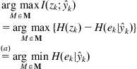
, i.e., ![]() . In this case, the MinMI criterion is equivalent to the MEE criterion. In fact, we can derive
. In this case, the MinMI criterion is equivalent to the MEE criterion. In fact, we can derive
 (6.4)
(6.4)
where (a) is because that the conditional entropy ![]() is not related to the parameter vector
is not related to the parameter vector ![]() . In Chapter 3, we have proved a similar property when discussing the MEE Bayesian estimation. That is, minimizing the estimation error entropy is equivalent to minimizing the mutual information between the error and the observation.
. In Chapter 3, we have proved a similar property when discussing the MEE Bayesian estimation. That is, minimizing the estimation error entropy is equivalent to minimizing the mutual information between the error and the observation.
Although both are equivalent, the MinMI criterion and the MEE criterion are much different in meaning. The former aims to decrease the statistical dependence while the latter tries to reduce the uncertainty (scatter or dispersion).
6.1.1 Properties of MinMI Criterion
Let the model be an FIR filter. We discuss in the following the optimal solution of the MinMI criterion and investigate the connection to the mean square error (MSE) criterion [234].
Theorem 6.1
For system identification scheme of Figure 6.1, if the model is an FIR filter (![]() ),
), ![]() and
and ![]() are zero-mean and jointly Gaussian, and the input covariance matrix
are zero-mean and jointly Gaussian, and the input covariance matrix ![]() satisfies
satisfies ![]() , then we have
, then we have ![]() , and
, and ![]() , where
, where ![]() ,
, ![]() denotes the optimal weight vector under MSE criterion.
denotes the optimal weight vector under MSE criterion.
Proof:
According to the mean square estimation theory [235], ![]() , thus we only need to prove
, thus we only need to prove ![]() . As
. As ![]() , we have
, we have
 (6.5)
(6.5)
where ![]() . And then, we can derive the following gradient
. And then, we can derive the following gradient
 (6.6)
(6.6)
where (a) follows from the fact that the conditional entropy ![]() does not depend on the weight vector
does not depend on the weight vector ![]() and (b) is because that
and (b) is because that ![]() is zero-mean Gaussian. Let this gradient be zero, we obtain
is zero-mean Gaussian. Let this gradient be zero, we obtain ![]() . Next we prove
. Next we prove ![]() . By (2.28), we have
. By (2.28), we have
 (6.7)
(6.7)
where (c) follows from ![]() .
.
Theorem 6.1 indicates that with Gaussian assumption, the optimal FIR filter under MinMI criterion will be equivalent to that under the MSE criterion (i.e., the Wiener solution), and the MinMI between the error and the input will be zero.
Theorem 6.2
If the unknown system and the model are both FIR filters with the same order, and the noise signal ![]() is independent of the input sequence
is independent of the input sequence ![]() (both can be of arbitrary distribution), then we have
(both can be of arbitrary distribution), then we have ![]() , where
, where ![]() denotes the weight vector of unknown system.
denotes the weight vector of unknown system.
Proof:
Without Gaussian assumption, Theorem 6.1 cannot be applied here. Let ![]() be the weight error vector between the unknown system and the model. We have
be the weight error vector between the unknown system and the model. We have ![]() and
and
 (6.8)
(6.8)
where (a) is due to the fact that the entropy of the sum of two independent random variables is not less than the entropy of each individual variable. The equality in (a) holds if and only if ![]() , i.e.,
, i.e., ![]() .
.
Theorem 6.2 suggests that the MinMI criterion might be robust with respect to the independent additive noise despite its distribution.
Theorem 6.3
Under the conditions of Theorem 6.2, and assuming that the input ![]() and the noise
and the noise ![]() are both unit-power white Gaussian processes, then
are both unit-power white Gaussian processes, then
![]() (6.9)
(6.9)
where ![]() ,
, ![]() ,
, ![]() ,
, ![]() .
.
Proof:
Obviously, we have ![]() , and
, and
![]() (6.10)
(6.10)
By the mean square estimation theory [235],
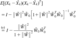 (6.11)
where (a) follows from ![]() ,
, ![]() is an
is an ![]() identity matrix. Therefore
identity matrix. Therefore
 (6.12)
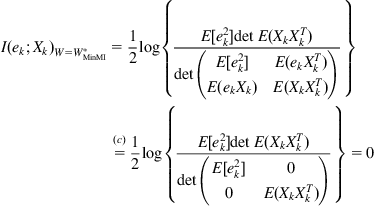
On the other hand, by (2.28), the mutual information ![]() can be calculated as
can be calculated as
 (6.13)
Combining (6.12) and (6.13) yields the result.
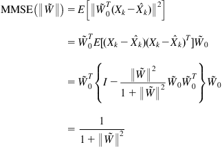
The term ![]() in Theorem 6.3 is actually the minimum MSE when estimating
in Theorem 6.3 is actually the minimum MSE when estimating ![]() based on
based on ![]() . Figure 6.2 shows the mutual information
. Figure 6.2 shows the mutual information ![]() and the minimum MSE
and the minimum MSE ![]() versus different weight error norm
versus different weight error norm ![]() . It can be seen that as
. It can be seen that as ![]() (or
(or ![]() ), we have
), we have ![]() and
and ![]() . This implies that when the model weight vector
. This implies that when the model weight vector ![]() approaches the system weight vector
approaches the system weight vector ![]() , the error
, the error ![]() contains less and less information about the input vector
contains less and less information about the input vector ![]() (or the information contained in the input signal has been sufficiently utilized), and it becomes more and more difficult to estimate the input based on the error signal (i.e., the minimum MSE
(or the information contained in the input signal has been sufficiently utilized), and it becomes more and more difficult to estimate the input based on the error signal (i.e., the minimum MSE ![]() attains gradually its maximum value).
attains gradually its maximum value).
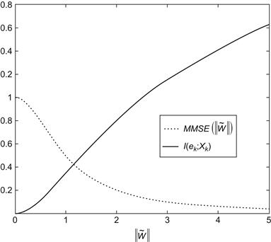
Figure 6.2 Mutual information ![]() and the minimum MSE
and the minimum MSE ![]() versus weight error norm. Source: Adopted from [234].
versus weight error norm. Source: Adopted from [234].
6.1.2 Relationship with Independent Component Analysis
The parameter identification under MinMI criterion is actually a special case of independent component analysis (ICA) [133]. A brief scheme of the ICA problem is shown in Figure 6.3, where ![]() is the
is the ![]() -dimensional source vector,
-dimensional source vector, ![]() is the
is the ![]() -dimensional observation vector that is related to the source vector through
-dimensional observation vector that is related to the source vector through ![]() , where
, where ![]() is the
is the ![]() mixing matrix [236]. Assume that each component of the source signal
mixing matrix [236]. Assume that each component of the source signal ![]() is mutually independent. There is no other prior knowledge about
is mutually independent. There is no other prior knowledge about ![]() and the mixing matrix
and the mixing matrix ![]() . The aim of the ICA is to search a
. The aim of the ICA is to search a ![]() matrix
matrix ![]() (i.e., the demixing matrix) such that
(i.e., the demixing matrix) such that ![]() approaches as closely as possible
approaches as closely as possible ![]() up to scaling and permutation ambiguities.
up to scaling and permutation ambiguities.
The ICA can be formulated as an optimization problem. To make each component of ![]() as mutually independent as possible, one can solve the matrix
as mutually independent as possible, one can solve the matrix ![]() under a certain objective function that measures the degree of dependence (or independence). Since the mutual information measures the statistical dependence between random variables, we may use the mutual information between components of
under a certain objective function that measures the degree of dependence (or independence). Since the mutual information measures the statistical dependence between random variables, we may use the mutual information between components of ![]() as the optimization criterion,2 i.e.,
as the optimization criterion,2 i.e.,
 (6.14)
To some extent, the system parameter identification can be regarded as an ICA problem. Consider the FIR system identification:
 (6.15)
where ![]() ,
, ![]() and
and ![]() are
are ![]() -dimensional weight vectors of the unknown system and the model. If regarding the vectors
-dimensional weight vectors of the unknown system and the model. If regarding the vectors ![]() and
and ![]() as, respectively, the source signal and the observation in ICA, we have
as, respectively, the source signal and the observation in ICA, we have
![]() (6.16)
(6.16)
where ![]() is the mixing matrix and
is the mixing matrix and ![]() is the
is the ![]() identity matrix. The goal of the parameter identification is to make the model weight vector
identity matrix. The goal of the parameter identification is to make the model weight vector ![]() approximate the unknown weight vector
approximate the unknown weight vector ![]() , and hence make the identification error
, and hence make the identification error ![]() (
(![]() ) approach the additive noise
) approach the additive noise ![]() , or in other words, make the vector
, or in other words, make the vector ![]() approach the ICA source vector
approach the ICA source vector ![]() . Therefore, the vector
. Therefore, the vector ![]() can be regarded as the demixing output vector, where the demixing matrix is
can be regarded as the demixing output vector, where the demixing matrix is
![]() (6.17)
(6.17)
Due to the scaling ambiguity of the demixing output, it is reasonable to introduce a more general demixing matrix:
![]() (6.18)
(6.18)
where ![]() ,
, ![]() . In this case, the demixed output
. In this case, the demixed output ![]() will be related to the identification error via a proportional factor
will be related to the identification error via a proportional factor ![]() .
.
According to (6.14), the optimal demixing matrix will be
 (6.19)
After obtaining the optimal matrix ![]() , one may get the optimal weight vector [133]
, one may get the optimal weight vector [133]
![]() (6.20)
(6.20)
Clearly, the above ICA formulation is actually the MinMI criterion-based parameter identification.
6.1.3 ICA-Based Stochastic Gradient Identification Algorithm
The MinMI criterion is in essence equivalent to the MEE criterion. Thus, one can utilize the various information gradient algorithms in Chapter 4 to implement the MinMI criterion-based identification. In the following, we introduce an ICA-based stochastic gradient identification algorithm [133].
According to the previous discussion, the MinMI criterion-based identification can be regarded as an ICA problem, i.e.,
![]() (6.21)
(6.21)
Since
![]() (6.22)
(6.22)
by (2.8), we have
![]() (6.23)
(6.23)
And hence
 (6.24)
where (a) is due to the fact that the term ![]() is not related to the matrix
is not related to the matrix ![]() . Denote the objective function
. Denote the objective function ![]() . The instantaneous value of
. The instantaneous value of ![]() is
is
![]() (6.25)
(6.25)
in which ![]() is the PDF of
is the PDF of ![]() (
(![]() ).
).
In order to solve the demixing matrix ![]() , one can resort to the natural gradient (or relative gradient)-based method [133,237]:
, one can resort to the natural gradient (or relative gradient)-based method [133,237]:
 (6.26)
where ![]() . As the PDF
. As the PDF ![]() is usually unknown, a certain nonlinear function (e.g., the tanh function) will be used to approximate the
is usually unknown, a certain nonlinear function (e.g., the tanh function) will be used to approximate the ![]() function.3
function.3
If adopting different step-sizes for learning the parameters ![]() and
and ![]() , we have
, we have
 (6.27)
The above algorithm is referred to as the ICA-based stochastic gradient identification algorithm (or simply the ICA algorithm). The model weight vector learned by this method is
![]() (6.28)
(6.28)
If the parameter ![]() is set to constant
is set to constant ![]() , the algorithm will reduce to
, the algorithm will reduce to
![]() (6.29)
(6.29)
6.1.4 Numerical Simulation Example
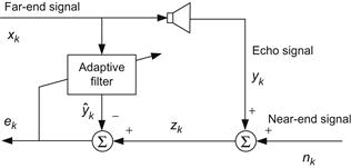
Figure 6.4 illustrates a general configuration of an acoustic echo canceller (AEC) [133]. ![]() is the far-end signal going to the loudspeaker, and
is the far-end signal going to the loudspeaker, and ![]() is the echo signal entering into the microphone that is produced by an undesirable acoustic coupling between the loudspeaker and the microphone.
is the echo signal entering into the microphone that is produced by an undesirable acoustic coupling between the loudspeaker and the microphone. ![]() is the near-end signal which is usually independent of the far-end signal and the echo signal.
is the near-end signal which is usually independent of the far-end signal and the echo signal. ![]() is the signal received by the microphone (
is the signal received by the microphone (![]() ). The aim of the echo cancelation is to remove the echo part in
). The aim of the echo cancelation is to remove the echo part in ![]() by subtracting the output of an adaptive filter that is driven by the far-end signal. As shown in Figure 6.4, the filter output
by subtracting the output of an adaptive filter that is driven by the far-end signal. As shown in Figure 6.4, the filter output ![]() is the synthetic echo signal, and the error signal
is the synthetic echo signal, and the error signal ![]() is the echo-canceled signal (or the estimate of the near-end signal). The key technique in AEC is to build an accurate model for the echo channel (or accurately identifying the parameters of the synthetic filter).
is the echo-canceled signal (or the estimate of the near-end signal). The key technique in AEC is to build an accurate model for the echo channel (or accurately identifying the parameters of the synthetic filter).
One may use the previously discussed ICA algorithm to implement the adaptive echo cancelation [133]. Suppose the echo channel is a 100 tap FIR filter, and assume that the input (far-end) signal ![]() is uniformly distributed over the interval [–4, 4], and the noise (near-end) signal
is uniformly distributed over the interval [–4, 4], and the noise (near-end) signal ![]() is Cauchy distributed, i.e.,
is Cauchy distributed, i.e., ![]() . The performance of the algorithms is measured by the echo return loss enhancement (ERLE) in dB:
. The performance of the algorithms is measured by the echo return loss enhancement (ERLE) in dB:
![]() (6.30)
(6.30)
Simulation results are shown in Figures 6.5 and 6.6. In Figure 6.5, the performances of the ICA algorithm, the normalized least mean square (NLMS), and the recursive least squares (RLS) are compared, while in Figure 6.6, the performances of the ICA algorithm and the algorithm (6.29) with ![]() are compared. During the simulation, the
are compared. During the simulation, the ![]() function in the ICA algorithm is chosen as
function in the ICA algorithm is chosen as
![]() (6.31)
(6.31)

Figure 6.5 Plots of the performance of three algorithms (ICA, NLMS, RLS) in Cauchy noise environment. Source: Adopted from [133].

Figure 6.6 Plots of the performance of the ICA algorithm and the algorithm (6.29) with ![]() (
(![]() ). Source: Adopted from [133].
). Source: Adopted from [133].
It can be clearly seen that the ICA-based algorithm shows excellent performance in echo cancelation.
6.2 System Identification Under the MaxMI Criterion
Consider the system identification scheme shown in Figure 6.7, in which ![]() is the common input to the unknown system and the model,
is the common input to the unknown system and the model, ![]() is the intrinsic (noiseless) output of the unknown system,
is the intrinsic (noiseless) output of the unknown system, ![]() is the additive noise,
is the additive noise, ![]() is the noisy output measurement, and
is the noisy output measurement, and ![]() stands for the output of the model. Under the MaxMI criterion, the identification procedure is to determine a model
stands for the output of the model. Under the MaxMI criterion, the identification procedure is to determine a model ![]() such that the mutual information between the noisy system output
such that the mutual information between the noisy system output ![]() and the model output
and the model output ![]() is maximized. Thus the optimal model
is maximized. Thus the optimal model ![]() is given by
is given by
 (6.32)
where ![]() denotes the model set (collection of all candidate models),
denotes the model set (collection of all candidate models), ![]() ,
, ![]() , and
, and ![]() denote, respectively, the PDFs of
denote, respectively, the PDFs of ![]() ,
, ![]() , and
, and ![]() .
.

The MaxMI criterion provides a fresh insight into system identification. Roughly speaking, the noisy measurement ![]() represents the output of an information source and is transmitted over an information channel, i.e., the identifier (including the model set and search algorithm), and the model output
represents the output of an information source and is transmitted over an information channel, i.e., the identifier (including the model set and search algorithm), and the model output ![]() represents the channel output. Then the identification problem can be regarded as the information transmitting problem, and the goal of identification is to maximize the channel capacity (measured by
represents the channel output. Then the identification problem can be regarded as the information transmitting problem, and the goal of identification is to maximize the channel capacity (measured by ![]() ) over all possible identifiers.
) over all possible identifiers.
6.2.1 Properties of the MaxMI Criterion
In the following, we present some important properties of the MaxMI criterion [135,136].
Property 6.1:
Maximizing the mutual information ![]() is equivalent to minimizing the conditional error entropy
is equivalent to minimizing the conditional error entropy ![]() , where
, where ![]() .
.
Proof:
It is easy to derive
 (6.33)
And hence
 (6.34)
where (a) is due to the fact that the model ![]() has no effect on the entropy
has no effect on the entropy ![]() .
.
The second property states that under certain conditions, the MaxMI criterion will be equivalent to maximizing the correlation coefficient.
Property 6.2:
If ![]() and
and ![]() are jointly Gaussian, we have
are jointly Gaussian, we have ![]() , where
, where ![]() is the correlation coefficient between
is the correlation coefficient between ![]() and
and ![]() .
.
Proof:
Since ![]() and
and ![]() are jointly Gaussian, the mutual information
are jointly Gaussian, the mutual information ![]() can be calculated as
can be calculated as
![]() (6.35)
(6.35)
The log function is monotonically increasing, thus we have
![]() (6.36)
(6.36)
Property 6.3:
Assume the noise ![]() is independent of the input signal
is independent of the input signal ![]() . Then maximizing the mutual information
. Then maximizing the mutual information ![]() is equivalent to maximizing a lower bound of the intrinsic (noiseless) mutual information
is equivalent to maximizing a lower bound of the intrinsic (noiseless) mutual information ![]() .
.
Proof:
Denote ![]() the intrinsic error, i.e.,
the intrinsic error, i.e., ![]() , we have
, we have
 (6.37)
where (b) follows from the independence condition and the fact that the entropy of the sum of two independent random variables is not less than the entropy of each individual variable. It follows easily that
![]() (6.38)
(6.38)
which completes the proof.
In Figure 6.7, the measurement ![]() may be further distorted by a certain function. Denote
may be further distorted by a certain function. Denote ![]() the distorted measurement, we have
the distorted measurement, we have
![]() (6.39)
(6.39)
where ![]() is the distortion function. Such distortion widely exists in practical systems. Typical examples include the saturation and the dead zone.
is the distortion function. Such distortion widely exists in practical systems. Typical examples include the saturation and the dead zone.
Property 6.4:
Suppose the noisy measurement ![]() is distorted by a function
is distorted by a function ![]() . Then maximizing the distorted mutual information,
. Then maximizing the distorted mutual information, ![]() is equivalent to maximizing a lower bound of the undistorted mutual information
is equivalent to maximizing a lower bound of the undistorted mutual information ![]() .
.
Proof:
This property is a direct consequence of the data processing inequality (see Theorem 2.3), which states that for any random variables ![]() and
and ![]() , and any measurable function
, and any measurable function ![]() ,
,
![]() (6.40)
(6.40)
In (6.40), if function ![]() is invertible, the equality will hold. In this case, we have
is invertible, the equality will hold. In this case, we have
![]() (6.41)
(6.41)
That is, the invertible distortion does not change the optimal solutions of MaxMI.
Property 6.5:
If the measurement ![]() is Gaussian, then maximizing the mutual information
is Gaussian, then maximizing the mutual information ![]() will be equivalent to minimizing a lower bound of the MSE.
will be equivalent to minimizing a lower bound of the MSE.
Proof:
According to Theorem 2.4, the rate distortion function for a Gaussian source ![]() with MSE distortion is
with MSE distortion is
![]() (6.42)
(6.42)
where ![]() . Let
. Let ![]() , we have
, we have
 (6.43)
where ![]() is the variance of
is the variance of ![]() . It follows easily that
. It follows easily that
 (6.44)
This completes the proof.
Consider now a special case where the model is represented by an FIR filter in which the output ![]() is given by
is given by
![]() (6.45)
(6.45)
where ![]() is the input (regressor) vector and
is the input (regressor) vector and ![]() is the weight vector. Then we have the following results.
is the weight vector. Then we have the following results.
Property 6.6:
For the case of the FIR model and under the assumption that ![]() and
and ![]() are jointly Gaussian, the optimal weight vector under the MaxMI criterion will be
are jointly Gaussian, the optimal weight vector under the MaxMI criterion will be
![]() (6.46)
(6.46)
where ![]() ,
, ![]() ,
, ![]() (
(![]() ). and in particular, if
). and in particular, if ![]() , the MSE
, the MSE ![]() will attain the lower bound as in (6.44), i.e.,
will attain the lower bound as in (6.44), i.e.,
![]() (6.47)
(6.47)
Proof:
Since ![]() and
and ![]() are jointly Gaussian, then
are jointly Gaussian, then ![]() and
and ![]() are also jointly Gaussian. By Property 6.2, we have
are also jointly Gaussian. By Property 6.2, we have
 (6.48)
where (c) is because that ![]() is not related to
is not related to ![]() . And then,
. And then,
 (6.49)
Let the above gradient be zero, and denote ![]() , we obtain the optimal weight vector
, we obtain the optimal weight vector
![]() (6.50)
(6.50)
It can be easily verified that for any ![]() , and
, and ![]() , the optimal weight vector (6.50) makes the gradient (6.49) zero. When
, the optimal weight vector (6.50) makes the gradient (6.49) zero. When ![]() , the optimal weight becomes the Wiener solution
, the optimal weight becomes the Wiener solution ![]() . In this case, the MSE is
. In this case, the MSE is
![]() (6.51)
(6.51)
Further the mutual information ![]() is
is
 (6.52)
Combining (6.51) and (6.52), we obtain ![]() .
.
Property 6.6 indicates that with a FIR filter structure and under Gaussian assumption, the MaxMI criterion yields a scaled Wiener solution which is not unique. Thus it does not satisfy the identifiability condition.4 The main reason for this is that any invertible transformation does not change the mutual information. In this property, ![]() is restricted to nonzero. If
is restricted to nonzero. If ![]() , we have
, we have ![]() , and the mutual information
, and the mutual information ![]() will be undefined (ill-posed).
will be undefined (ill-posed).
A priori information usually has great value in system identification. For example, if the structures of the system or the parameters are partially known, we may use this information to impose some constraints on the structures or parameters of the filter. For the case in which the desired responses are distorted, the a priori information can help to improve the accuracy of the solution. In particular, certain parameter constraints may yield a unique optimal solution under the MaxMI criterion. Consider the optimal solution (6.50) under the following parameter constraint:
![]() (6.53)
(6.53)
where ![]() ,
, ![]() . Let
. Let ![]() , we have
, we have
![]() (6.54)
(6.54)
If ![]() , then
, then ![]() can be uniquely determined as
can be uniquely determined as ![]() .
.
6.2.2 Stochastic Mutual Information Gradient Identification Algorithm
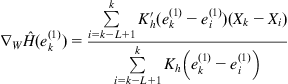
The stochastic gradient identification algorithm under the MaxMI criterion can be expressed as
![]() (6.55)
(6.55)
where ![]() denotes the instantaneous estimate of the gradient of mutual information
denotes the instantaneous estimate of the gradient of mutual information ![]() evaluated at the current value of the weight vector and
evaluated at the current value of the weight vector and ![]() is the step-size. The key problem of the update equation (6.55) is how to calculate the instantaneous gradient
is the step-size. The key problem of the update equation (6.55) is how to calculate the instantaneous gradient ![]() .
.
Let us start with the calculation of the gradient (not the instantaneous gradient) of ![]() :
:
 (6.56)
where ![]() ,
, ![]() , and
, and ![]() denote the related PDFs at the instant
denote the related PDFs at the instant ![]() . Then the instantaneous value of
. Then the instantaneous value of ![]() can be obtained by dropping the expectation operator and plugging in the estimates of the PDFs, i.e.,
can be obtained by dropping the expectation operator and plugging in the estimates of the PDFs, i.e.,
 (6.57)
where ![]() and
and ![]() are, respectively, the estimates of
are, respectively, the estimates of ![]() and
and ![]() . To estimate the density functions, one usually adopts the kernel density estimation (KDE) method and uses the following Gaussian functions as the kernels [135]
. To estimate the density functions, one usually adopts the kernel density estimation (KDE) method and uses the following Gaussian functions as the kernels [135]
 (6.58)
where ![]() and
and ![]() denote the kernel widths.
denote the kernel widths.
Based on the above Gaussian kernels, the estimates of the PDFs and their gradients can be calculated as follows:
 (6.59)
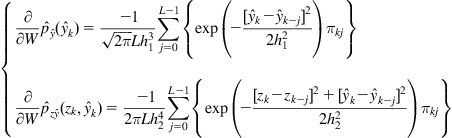 (6.60)
where ![]() is the sliding data length and
is the sliding data length and ![]() . For FIR filter, we have
. For FIR filter, we have
![]() (6.61)
(6.61)
Combining (6.55), (6.57), (6.59), and (6.60), we obtain a stochastic gradient identification algorithm under the MaxMI criterion, which is referred to as the stochastic mutual information gradient (SMIG) algorithm [135].
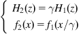
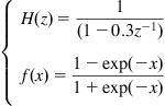
The performances of the SMIG algorithm compared with the least mean square (LMS) algorithm are demonstrated in the following by Monte Carlo simulations. Consider the FIR system identification [135]:
 (6.62)
where ![]() and
and ![]() are, respectively, the transfer functions of the unknown system and the model. Suppose the input signal
are, respectively, the transfer functions of the unknown system and the model. Suppose the input signal ![]() and the additive noise
and the additive noise ![]() are both unit-power white Gaussian processes. To uniquely determine an optimal solution under the MaxMI criterion, it is assumed that the first component of the unknown weight vector is a priori known (which is assumed to be 0.8). Thus the goal is to search the optimal solution of the other five weights. The initial weights (except
are both unit-power white Gaussian processes. To uniquely determine an optimal solution under the MaxMI criterion, it is assumed that the first component of the unknown weight vector is a priori known (which is assumed to be 0.8). Thus the goal is to search the optimal solution of the other five weights. The initial weights (except ![]() ) for the adaptive FIR filter are zero-mean Gaussian distributed with variance 0.01. Further, the following distortion functions are considered [135]:
) for the adaptive FIR filter are zero-mean Gaussian distributed with variance 0.01. Further, the following distortion functions are considered [135]:


Figure 6.8 plots the distortion functions of the saturation and dead zone. Figure 6.9 shows the desired response signal with data loss (the probability of data loss is 0.3). In the simulation below, the Gaussian kernels are used and the kernel sizes are kept fixed at ![]() .
.

Figure 6.8 Distortion functions of saturation and dead zone. Source: Adopted from [135].

Figure 6.9 Desired response signal with data loss. Source: Adopted from [135].
Figure 6.10 illustrates the average convergence curves over 50 Monte Carlo simulation runs. One can see that, without measurement distortions, the conventional LMS algorithm has a better performance. However, in the case of measurement distortions, it is evident the deterioration of the LMS algorithm whereas the SMIG algorithm is little affected and achieves a much better performance. Simulation results confirm that the MaxMI criterion is more robust to the measurement distortion than traditional MSE criterion.

Figure 6.10 Average convergence curves of SMIG and LMS algorithms: (A) undistorted, (B) saturation, (C) dead zone, and (D) data loss. Source: Adopted from [135].
6.2.3 Double-Criterion Identification Method
The system identification scheme of Figure 6.7 does not, in general, satisfy the condition of parameter identifiability (i.e., the uniqueness of the optimal solution). In order to uniquely determine an optimal solution, some a priori information about the parameters is required. However, such a priori information is not available for many practical applications. To address this problem, we introduce in the following the double-criterion identification method [136].
Consider the Wiener system shown in Figure 6.11, where the system has the cascade structure and consists of a discrete-time linear filter ![]() followed by a zero-memory nonlinearity
followed by a zero-memory nonlinearity ![]() . Wiener systems are typical nonlinear systems and are widely used for nonlinear modeling [238]. The double-criterion method mainly aims at the Wiener system identification, but it also applies to many other systems. In fact, any system can be regarded as a cascade system consisting of itself followed by
. Wiener systems are typical nonlinear systems and are widely used for nonlinear modeling [238]. The double-criterion method mainly aims at the Wiener system identification, but it also applies to many other systems. In fact, any system can be regarded as a cascade system consisting of itself followed by ![]() .
.
First, we define the equivalence between two Wiener systems.
Definition 6.1
Two Wiener systems ![]() and
and ![]() are said to be equivalent if and only if
are said to be equivalent if and only if ![]() , such that
, such that
 (6.63)
Although there is a scale factor ![]() between two equivalent Wiener systems, they have exactly the same input–output behavior.
between two equivalent Wiener systems, they have exactly the same input–output behavior.
The optimal solution of the system identification scheme of Figure 6.7 is usually nonunique. For Wiener system, the nonuniqueness means the optimal solutions are not all equivalent. According to the data processing inequality, we have
![]() (6.64)
(6.64)
where ![]() and
and ![]() denote, respectively, the intermediate output (the output of the linear part) and the zero-memory nonlinearity of the Wiener model. Then under the MaxMI criterion, the optimal Wiener model will be
denote, respectively, the intermediate output (the output of the linear part) and the zero-memory nonlinearity of the Wiener model. Then under the MaxMI criterion, the optimal Wiener model will be
 (6.65)
where ![]() denotes the parameter vector of the linear subsystem and
denotes the parameter vector of the linear subsystem and ![]() denotes all measurable mappings
denotes all measurable mappings ![]() . Evidently, the optimal solutions given by (6.65) contain infinite nonequivalent Wiener models. Actually, we always have
. Evidently, the optimal solutions given by (6.65) contain infinite nonequivalent Wiener models. Actually, we always have ![]() provided
provided ![]() is an invertible function.
is an invertible function.
In order to ensure that all the optimal Wiener models are equivalent, the identification scheme of Figure 6.7 has to be modified. One can adopt the double-criterion identification method [136]. As shown in Figure 6.12, the double-criterion method utilizes both MaxMI and MSE criteria to identify the Wiener system. Specifically, the linear filter part is identified by using the MaxMI criterion, and the zero-memory nonlinear part is learned by the MSE criterion. In Figure 6.12, ![]() and
and ![]() denote, respectively, the linear and nonlinear subsystems of the unknown Wiener system, where
denote, respectively, the linear and nonlinear subsystems of the unknown Wiener system, where ![]() and
and ![]() are related parameter vectors. The adaptive Wiener model
are related parameter vectors. The adaptive Wiener model ![]() usually takes the form of “FIR + polynomial”, that is, the linear subsystem
usually takes the form of “FIR + polynomial”, that is, the linear subsystem ![]() is an
is an ![]() -order FIR filter, and the nonlinear subsystem
-order FIR filter, and the nonlinear subsystem ![]() is a
is a ![]() -order polynomial. In this case, the intermediate output
-order polynomial. In this case, the intermediate output ![]() and the final output
and the final output ![]() of the model are
of the model are
 (6.66)
where ![]() and
and ![]() are
are ![]() -dimensional FIR weight vector and input vector,
-dimensional FIR weight vector and input vector, ![]() is the
is the ![]() -dimensional polynomial coefficient vector, and
-dimensional polynomial coefficient vector, and ![]() is the polynomial basis vector.
is the polynomial basis vector.
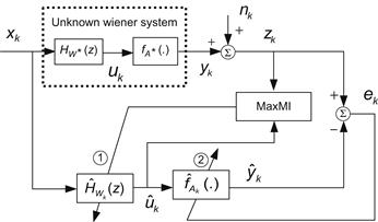
Figure 6.12 Double-criterion identification scheme for Wiener system: (1) linear filter part is identified using MaxMI criterion and (2) nonlinear part is trained using MSE criterion.
It should be noted that similar two-gradient identification algorithms for the Wiener system have been proposed in [239,240], wherein the linear and nonlinear subsystems are both identified using the MSE criterion.
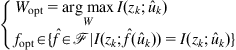
The optimal solution for the above double-criterion identification is
 (6.67)
For general case, it is hard to find the closed-form expressions for ![]() and
and ![]() . The following theorem only considers the case in which the unknown Wiener system has the same structure as the assumed Wiener model.
. The following theorem only considers the case in which the unknown Wiener system has the same structure as the assumed Wiener model.
Theorem 6.4
For the Wiener system identification scheme shown in Figure 6.12, if
1. The unknown system and the model have the same structure, that is, ![]() and
and ![]() are both
are both ![]() -order FIR filters, and
-order FIR filters, and ![]() and
and ![]() are both
are both ![]() -order polynomials.
-order polynomials.
Then the optimal solution of (6.67) will be
![]() (6.68)
(6.68)
where ![]() ,
, ![]() , and
, and ![]() is expressed as
is expressed as
 (6.69)
Proof:
Since ![]() and
and ![]() are mutually independent, we have
are mutually independent, we have
 (6.70)
where ![]() follows from the fact that the entropy of the sum of two independent random variables is not less than the entropy of each individual variable.
follows from the fact that the entropy of the sum of two independent random variables is not less than the entropy of each individual variable.
In (6.70), the equality holds if and only if conditioned on ![]() ,
, ![]() is a deterministic variable, that is,
is a deterministic variable, that is, ![]() is a function of
is a function of ![]() . This implies that the mutual information
. This implies that the mutual information ![]() will achieve its maximum value (
will achieve its maximum value (![]() ) if and only if there exists a function
) if and only if there exists a function ![]() such that
such that ![]() , i.e.,
, i.e.,
![]() (6.71)
(6.71)
As the nonlinear function ![]() is assumed to be invertible, we have
is assumed to be invertible, we have
![]() (6.72)
(6.72)
where ![]() denotes the inverse function of
denotes the inverse function of ![]() and
and ![]() . It follows that
. It follows that
 (6.73)
And hence
![]() (6.74)
(6.74)
which implies ![]() . Let
. Let ![]() , we obtain the optimum FIR weight
, we obtain the optimum FIR weight ![]() .
.
Now the optimal polynomial coefficients can be easily determined. By independent assumption, we have
![]() (6.75)
(6.75)
with equality if and only if ![]() . This means the MSE cost will attain its minimum value (
. This means the MSE cost will attain its minimum value (![]() ) if and only if the intrinsic error (
) if and only if the intrinsic error (![]() ) remains zero. Therefore,
) remains zero. Therefore,
 (6.76)
Then we get ![]() , where
, where ![]() is given by (6.69). This completes the proof.
is given by (6.69). This completes the proof.
Theorem 6.4 indicates that for identification scheme of Figure 6.12, under certain conditions the optimal solution will match the true system exactly (i.e., with zero intrinsic error). There is a free parameter ![]() in the solution, however, its specific value has no substantial effect on the cascaded model. The literature [240] gives a similar result about the optimal solution under the single MSE criterion. In [240], the linear FIR subsystem is estimated up to a scaling factor which equals the derivative of the nonlinear function around a bias point.
in the solution, however, its specific value has no substantial effect on the cascaded model. The literature [240] gives a similar result about the optimal solution under the single MSE criterion. In [240], the linear FIR subsystem is estimated up to a scaling factor which equals the derivative of the nonlinear function around a bias point.
The double-criterion identification can be implemented in two manners. The first is the sequential identification scheme, in which the MaxMI criterion is first used to learn the linear FIR filter. At the end of the first adaptation phase, the tap weights are frozen, and then the MSE criterion is used to estimate the polynomial coefficients. The second adaptation scheme simultaneously trains both the linear and nonlinear parts of the Wiener model. Obviously, the second scheme is more suitable for online identification. In the following, we focus only on the simultaneous scheme.
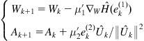
In [136], a stochastic gradient-based double-criterion identification algorithm was developed as follows:
 (6.77)
where ![]() denotes the stochastic (instantaneous) gradient of the mutual information
denotes the stochastic (instantaneous) gradient of the mutual information ![]() with respect to the FIR weight vector
with respect to the FIR weight vector ![]() (see (6.57) for the computation),
(see (6.57) for the computation), ![]() denotes the Euclidean norm,
denotes the Euclidean norm, ![]() and
and ![]() are the step-sizes. The update equation (a1) is actually the SMIG algorithm developed in 6.2.2. The second part (a2) of the algorithm (6.77) scales the FIR weight vector to a unit vector. The purpose of scaling the weight vector is to constrain the output energy of the FIR filter, and to avoid “very large values” of the scale factor
are the step-sizes. The update equation (a1) is actually the SMIG algorithm developed in 6.2.2. The second part (a2) of the algorithm (6.77) scales the FIR weight vector to a unit vector. The purpose of scaling the weight vector is to constrain the output energy of the FIR filter, and to avoid “very large values” of the scale factor ![]() in the optimal solution. As mutual information is scaling invariant,6 the scaling (a2) does not influence the search of the optimal solution. However, it certainly affects the value of
in the optimal solution. As mutual information is scaling invariant,6 the scaling (a2) does not influence the search of the optimal solution. However, it certainly affects the value of ![]() in the optimal solution. In fact, if the algorithm converges to the optimal solution, we have
in the optimal solution. In fact, if the algorithm converges to the optimal solution, we have ![]() , and
, and
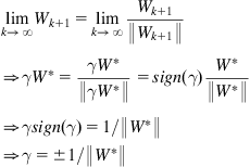 (6.78)
That is, the scale factor ![]() equals either
equals either ![]() or
or ![]() , which is no longer a free parameter.
, which is no longer a free parameter.
The third part (a3) of the algorithm (6.77) is the NLMS algorithm, which minimizes the MSE cost with step-size scaled by the energy of polynomial regression signal ![]() . The NLMS is more suitable for the nonlinear subsystem identification than the standard LMS algorithm, because during the adaptation, the polynomial regression signals are usually nonstationary. The algorithm (6.77) is referred to as the SMIG-NLMS algorithm [136].
. The NLMS is more suitable for the nonlinear subsystem identification than the standard LMS algorithm, because during the adaptation, the polynomial regression signals are usually nonstationary. The algorithm (6.77) is referred to as the SMIG-NLMS algorithm [136].
Next, Monte Carlo simulation results are presented to demonstrate the performance of the SMIG-NLMS algorithm. For comparison purpose, simulation results of the following two algorithms are also included.
 (6.79)
 (6.80)
where ![]() ,
, ![]() ,
, ![]() ,
, ![]() are step-sizes,
are step-sizes, ![]() ,
, ![]() , and
, and ![]() denote the stochastic information gradient (SIG) under Shannon entropy criterion, calculated as
denote the stochastic information gradient (SIG) under Shannon entropy criterion, calculated as
 (6.81)
where ![]() denotes the kernel function with bandwidth
denotes the kernel function with bandwidth ![]() . The algorithms (6.79) and (6.80) are referred to as the LMS-NLMS and SIG-NLMS algorithms [136], respectively. Note that the LMS-NLMS algorithm is actually the normalized version of the algorithm developed in [240].
. The algorithms (6.79) and (6.80) are referred to as the LMS-NLMS and SIG-NLMS algorithms [136], respectively. Note that the LMS-NLMS algorithm is actually the normalized version of the algorithm developed in [240].
Due to the “scaling” property of the linear and nonlinear portions, the expression of Wiener system is not unique. In order to evaluate how close the estimated Wiener model and the true system are, we introduce the following measures [136]:

Among the three performance measures, the angles ![]() and
and ![]() quantify the identification performance of the subsystems (linear FIR and nonlinear polynomial), while the IEP quantifies the overall performance.
quantify the identification performance of the subsystems (linear FIR and nonlinear polynomial), while the IEP quantifies the overall performance.
Let us consider the case in which the FIR weights and the polynomial coefficients of the unknown Wiener system are [136]
![]() (6.86)
(6.86)
The common input ![]() is a white Gaussian process with unit variance and the disturbance noise
is a white Gaussian process with unit variance and the disturbance noise ![]() is another white Gaussian process with variance
is another white Gaussian process with variance ![]() . The initial FIR weight vector
. The initial FIR weight vector ![]() of the adaptive model is obtained by normalizing a zero-mean Gaussian-distributed random vector (
of the adaptive model is obtained by normalizing a zero-mean Gaussian-distributed random vector (![]() ), and the initial polynomial coefficients are zero-mean Gaussian distributed with variance 0.01. For the SMIG-NLMS and SIG-NLMS algorithms, the sliding data length is set as
), and the initial polynomial coefficients are zero-mean Gaussian distributed with variance 0.01. For the SMIG-NLMS and SIG-NLMS algorithms, the sliding data length is set as ![]() and the kernel widths are chosen according to Silverman’s rule. The step-sizes involved in the algorithms are experimentally selected so that the initial convergence rates are visually identical.
and the kernel widths are chosen according to Silverman’s rule. The step-sizes involved in the algorithms are experimentally selected so that the initial convergence rates are visually identical.
The average convergence curves of the angles ![]() and
and ![]() , over 1000 independent Monte Carlo simulation runs, are shown in Figures 6.13 and 6.14. It is evident that the SMIG-NLMS algorithm achieves the smallest angles (mismatches) in both linear and nonlinear subsystems during the steady-state phase. More detailed statistical results of the subsystems training are presented in Figures 6.15 and 6.16, in which the histograms of the angles
, over 1000 independent Monte Carlo simulation runs, are shown in Figures 6.13 and 6.14. It is evident that the SMIG-NLMS algorithm achieves the smallest angles (mismatches) in both linear and nonlinear subsystems during the steady-state phase. More detailed statistical results of the subsystems training are presented in Figures 6.15 and 6.16, in which the histograms of the angles ![]() and
and ![]() at the final iteration are plotted. The inset plots in Figures 6.15 and 6.16 give the summary of the mean and spread of the histograms. One can observe again that the SMIG-NLMS algorithm outperforms both the LMS-NLMS and SIG-NLMS algorithms in terms of the angles between the estimated and true parameter vectors.
at the final iteration are plotted. The inset plots in Figures 6.15 and 6.16 give the summary of the mean and spread of the histograms. One can observe again that the SMIG-NLMS algorithm outperforms both the LMS-NLMS and SIG-NLMS algorithms in terms of the angles between the estimated and true parameter vectors.

Figure 6.13 Average convergence curves of the angle ![]() over 1000 Monte Carlo runs. Source: Adopted from [136].
over 1000 Monte Carlo runs. Source: Adopted from [136].

Figure 6.14 Average convergence curves of the angle ![]() over 1000 Monte Carlo runs. Source: Adopted from [136].
over 1000 Monte Carlo runs. Source: Adopted from [136].

Figure 6.15 Histogram plots of the angle ![]() at the final iteration over 1000 Monte Carlo runs. Source: Adopted from [136].
at the final iteration over 1000 Monte Carlo runs. Source: Adopted from [136].
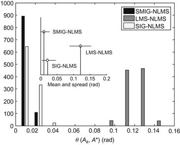
Figure 6.16 Histogram plots of the angle ![]() at the final iteration over 1000 Monte Carlo runs. Source: Adopted from [136].
at the final iteration over 1000 Monte Carlo runs. Source: Adopted from [136].
The overall identification performance can be measured by the IEP. Figure 6.17 illustrates the convergence curves of the IEP over 1000 Monte Carlo runs. It is clear that the SMIG-NLMS algorithm achieves the smallest IEP during the steady-state phase. Figure 6.18 shows the probability density functions of the steady-state intrinsic errors. As expected, the SMIG-NLMS algorithm yields the largest and most concentrated peak centered at the zero intrinsic error, and hence achieves the best accuracy in identification.

Figure 6.17 Convergence curves of the IEP over 1000 Monte Carlo runs. Source: Adopted from [136].
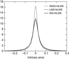
Figure 6.18 Probability density functions of the steady-state intrinsic errors. Source: Adopted from [136].
In the previous simulations, the unknown Wiener system has the same structure as the assumed model. In order to show how the algorithm performs when the real system is different from the assumed model (i.e., the unmatched case), another simulation with the same setup is conducted. This time the linear and nonlinear parts of the unknown system are assumed to be
 (6.87)
Table 6.1 lists the mean±deviation results of the IEP at final iteration over 1000 Monte Carlo runs. Clearly, the SMIG-NLMS algorithm produces the IEP with both lower mean and smaller deviation. Figure 6.19 shows the desired output (intrinsic output of the true system) and the model outputs (trained by different algorithms) during the last 100 samples for the test input. The results indicate that the identified model by the SMIG-NLMS algorithm describes the test data with the best accuracy.
Table 6.1
Mean±Deviation Results of the IEP at the Final Iteration Over 1000 Monte Carlo Runs
| IEP | |
| SMIG-NLMS | 0.0011±0.0065 |
| LMS-NLMS | 0.0028±0.0074 |
| SIG-NLMS | 0.0033±0.0089 |
Source: Adopted from [136].

Figure 6.19 Desired output (the intrinsic output of the true system) and model outputs for the test input data. Source: Adopted from [136].
Appendix I MinMI Rate Criterion
The authors in [124] propose the MinMI rate criterion. Consider the linear Gaussian system
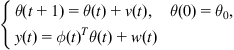 (I.1)
(I.1)
where ![]() ,
, ![]() ,
, ![]() . One can adopt the following linear recursive algorithm to estimate the parameters
. One can adopt the following linear recursive algorithm to estimate the parameters
![]() (I.2)
(I.2)
The MinMI rate criterion is to search an optimal gain matrix ![]() such that the mutual information rate
such that the mutual information rate ![]() between the error signal
between the error signal ![]() and a unity-power white Gaussian noise
and a unity-power white Gaussian noise ![]() is minimized, where
is minimized, where ![]() ,
, ![]() is a certain Gaussian process independent of
is a certain Gaussian process independent of ![]() . Clearly, the MinMI rate criterion requires that the asymptotic power spectral
. Clearly, the MinMI rate criterion requires that the asymptotic power spectral ![]() of the error process
of the error process ![]() satisfies
satisfies ![]() (otherwise
(otherwise ![]() does not exist). It can be calculated that
does not exist). It can be calculated that
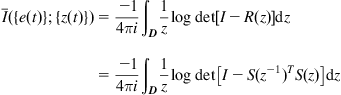 (I.3)
(I.3)
where ![]() is a spectral factor of
is a spectral factor of ![]() . Hence, under the MinMI rate criterion the optimal gain matrix
. Hence, under the MinMI rate criterion the optimal gain matrix ![]() will be
will be
![]() (I.4)
(I.4)
1The minimum mutual information rate criterion was also proposed in [124], which minimizes the mutual information rate between the error signal and a certain white Gaussian process (see Appendix I).
2The mutual information minimization is a basic optimality criterion in ICA. Other ICA criteria, such as the negentropy maximization, Infomax, likelihood maximization, and the higher order statistics, in general conform with the mutual information minimization.
3One can also apply the kernel density estimation method to estimate ![]() , and then use the estimated PDF to compute the
, and then use the estimated PDF to compute the ![]() function.
function.
4It is worth noting that the identifiability problem under the MaxMI criterion has been studied in [134], wherein the “identifiability” does not means the uniqueness of the solution, but just means that the mutual information between the system output and the model output is nonzero.
5Data loss means that there exists accidental loss of the measurement data due to certain failures in the sensors or communication channels.
6For any random variables ![]() and
and ![]() , the mutual information
, the mutual information ![]() satisfies
satisfies ![]() ,
, ![]() ,
, ![]() .
.
7In practice, the IEP is evaluated using the sample mean instead of the expectation value.