
System Identification Under Information Divergence Criteria
The fundamental contribution of information theory is to provide a unified framework for dealing with the notion of information in a precise and technical sense. Information, in a technical sense, can be quantified in a unified manner by using the Kullback–Leibler information divergence (KLID). Two information measures, Shannon’s entropy and mutual information are special cases of KL divergence [43]. The use of probability in system identification is also shown to be equivalent to measuring KL divergence between the actual and model distributions. In parameter estimation, the KL divergence for inference is consistent with common statistical approaches, such as the maximum likelihood (ML) estimation. Based on the KL divergence, Akaike derived the well-known Akaike’s information criterion (AIC), which is widely used in the area of model selection. Another important model selection criterion, the minimum description length, first proposed by Rissanen in 1978, is also closely related to the KL divergence. In identification of stationary Gaussian processes, it has been shown that the optimal solution to an approximation problem for Gaussian random variables with the divergence criterion is identical to the main step of the subspace algorithm [123].
There are many definitions of information divergence, but in this chapter our focus is mainly on the KLID. In most cases, the extension to other definitions is straightforward.
5.1 Parameter Identifiability Under KLID Criterion
The identifiability arises in the context of system identification, indicating whether or not the unknown parameter can be uniquely identified from the observation of the system. One would not select a model structure whose parameters cannot be identified, so the problem of identifiability is crucial in the procedures of system identification. There are many concepts of identifiability. Typical examples include Fisher information–based identifiability [216], least squares (LS) identifiability [217], consistency-in-probability identifiability [218], transfer function–based identifiability [219], and spectral density–based identifiability [219]. In the following, we discuss the fundamental problem of system parameter identifiability under KLID criterion.
5.1.1 Definitions and Assumptions
Let ![]() (
(![]() ) be a sequence of observations with joint probability density functions (PDFs)
) be a sequence of observations with joint probability density functions (PDFs) ![]() ,
, ![]() , where
, where ![]() is a
is a ![]() -dimensional column vector,
-dimensional column vector, ![]() is a
is a ![]() -dimensional parameter vector, and
-dimensional parameter vector, and ![]() is the parameter space. Let
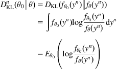
is the parameter space. Let ![]() be the true parameter. The KLID between
be the true parameter. The KLID between ![]() and
and ![]() will be
will be
 (5.1)
(5.1)
where ![]() denotes the expectation of the bracketed quantity taken with respect to the actual parameter value
denotes the expectation of the bracketed quantity taken with respect to the actual parameter value ![]() . Based on the KLID, a natural way of parameter identification is to look for a parameter
. Based on the KLID, a natural way of parameter identification is to look for a parameter ![]() , such that the KLID of Eq. (5.1) is minimized, that is,
, such that the KLID of Eq. (5.1) is minimized, that is,
![]() (5.2)
(5.2)
An important question that arises in the context of such identification problem is whether or not the parameter ![]() can be uniquely determined. This is the parameter identifiability problem. Assume
can be uniquely determined. This is the parameter identifiability problem. Assume ![]() lies in
lies in ![]() (hence
(hence ![]() ). The notion of identifiability under KLID criterion can then be defined as follows.
). The notion of identifiability under KLID criterion can then be defined as follows.
Definition 5.1
The parameter set ![]() is said to be KLID-identifiable at
is said to be KLID-identifiable at ![]() , if and only if
, if and only if ![]() ,
, ![]() ,
, ![]() implies
implies ![]() .
.
By the definition, if parameter set ![]() is KLID-identifiable at
is KLID-identifiable at ![]() (we also say
(we also say ![]() is KLID-identifiable), then for any
is KLID-identifiable), then for any ![]() ,
, ![]() , we have
, we have ![]() , and hence
, and hence ![]() . Therefore, any change in the parameter yields changes in the output density.
. Therefore, any change in the parameter yields changes in the output density.
The identifiability can also be defined in terms of the information divergence rate.
Definition 5.2
The parameter set ![]() is said to be KLIDR-identifiable at
is said to be KLIDR-identifiable at ![]() , if and only if
, if and only if ![]() , the KL information divergence rate (KLIDR)
, the KL information divergence rate (KLIDR) ![]() exists, and
exists, and ![]() implies
implies ![]() .
.
Let ![]() be the
be the ![]() -neighborhood of
-neighborhood of ![]() , where
, where ![]() denotes the Euclidean norm. The local KLID (or local KLIDR)-identifiability is defined as follows.
denotes the Euclidean norm. The local KLID (or local KLIDR)-identifiability is defined as follows.
Definition 5.3
The parameter set ![]() is said to be locally KLID (or locally KLIDR)-identifiable at
is said to be locally KLID (or locally KLIDR)-identifiable at ![]() , if and only if there exists
, if and only if there exists ![]() , such that
, such that ![]() ,
, ![]() (or
(or ![]() ) implies
) implies ![]() .
.
Here, we give some assumptions that will be used later on.
Assumption 5.1
![]() ,
, ![]() , the KLID
, the KLID ![]() always exists.
always exists.
Remark:
Let ![]() be the probability space of the output sequence
be the probability space of the output sequence ![]() with parameter
with parameter ![]() , where
, where ![]() is the related measurable space, and
is the related measurable space, and ![]() is the probability measure.
is the probability measure. ![]() is said to be absolutely continuous with respect to
is said to be absolutely continuous with respect to ![]() , denoted by
, denoted by ![]() , if
, if ![]() for every
for every ![]() such that
such that ![]() . Clearly, the existence of
. Clearly, the existence of ![]() implies
implies ![]() . Thus by Assumption 5.1,
. Thus by Assumption 5.1, ![]() , we have
, we have ![]() ,
, ![]() .
.
Assumption 5.2
The density function ![]() is at least twice continuously differentiable with respect to
is at least twice continuously differentiable with respect to ![]() , and
, and ![]() , the following interchanges between integral (or limitation) and derivative are permissible:
, the following interchanges between integral (or limitation) and derivative are permissible:
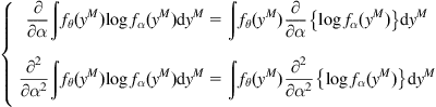 (5.3)
(5.3)
 (5.4)
(5.4)
Remark:
The interchange of differentiation and integration can be justified by bounded convergence theorem for appropriately well-behaved PDF ![]() . Similar assumptions can be found in Ref. [220]. A sufficient condition for the permission of interchange between differentiation and limitation is the uniform convergence of the limitation in
. Similar assumptions can be found in Ref. [220]. A sufficient condition for the permission of interchange between differentiation and limitation is the uniform convergence of the limitation in ![]() .
.
5.1.2 Relations with Fisher Information
Fisher information is a classical criterion for parameter identifiability [216]. There are close relationships between KLID (KLIDR)-identifiability and Fisher information.
The Fisher information matrix (FIM) for the family of densities ![]() is given by:
is given by:
 (5.5)
(5.5)
As ![]() , the Fisher information rate matrix (FIRM) is:
, the Fisher information rate matrix (FIRM) is:
![]() (5.6)
(5.6)
Theorem 5.1
Assume that ![]() is an open subset of
is an open subset of ![]() . Then,
. Then, ![]() will be locally KLID-identifiable if the FIM
will be locally KLID-identifiable if the FIM ![]() is positive definite.
is positive definite.
Proof:
As ![]() is an open subset, an obvious sufficient condition for
is an open subset, an obvious sufficient condition for ![]() to be locally KLID-identifiable is that
to be locally KLID-identifiable is that ![]() , and
, and ![]() . This can be easily proved. By Assumption 5.2, we have
. This can be easily proved. By Assumption 5.2, we have
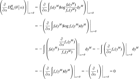 (5.7)
(5.7)
On the other hand, we can derive
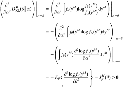 (5.8)
(5.8)
Theorem 5.2
Assume that ![]() is an open subset of
is an open subset of ![]() . Then
. Then ![]() will be locally KLIDR-identifiable if the FIRM
will be locally KLIDR-identifiable if the FIRM ![]() is positive definite.
is positive definite.
Proof:
By Theorem 5.1 and Assumption 5.2, we have
 (5.9)
(5.9)
and
 (5.10)
Thus, ![]() is locally KLIDR-identifiable.
is locally KLIDR-identifiable.
Suppose the observation sequence ![]() (
(![]() ) is a stationary zero-mean Gaussian process, with power spectral
) is a stationary zero-mean Gaussian process, with power spectral ![]() . According to Theorem 2.7, the spectral expressions of the KLIDR and FIRM are as follows:
. According to Theorem 2.7, the spectral expressions of the KLIDR and FIRM are as follows:
![]() (5.11)
(5.11)
![]() (5.12)
(5.12)
In this case, we can easily verify that ![]() , and
, and ![]() . In fact, we have
. In fact, we have
 (5.13)
and
 (5.14)
where  .
.
5.1.3 Gaussian Process Case
When the observation sequence ![]() is jointly Gaussian distributed, the KLID-identifiability can be easily checked. Consider the following joint Gaussian PDF:
is jointly Gaussian distributed, the KLID-identifiability can be easily checked. Consider the following joint Gaussian PDF:
![]() (5.15)
(5.15)
where ![]() is the mean vector, and
is the mean vector, and ![]() is the
is the ![]() -dimensional covariance matrix. Then we have
-dimensional covariance matrix. Then we have
![]() (5.16)
(5.16)
where ![]() is
is
 (5.17)
Clearly, for the Gaussian process ![]() , we have
, we have ![]() if and only if
if and only if ![]() and
and ![]() . Denote
. Denote ![]() ,
, ![]() , where
, where ![]() is the ith row and jth column element of
is the ith row and jth column element of ![]() . The element
. The element ![]() is said to be a regular element if and only if
is said to be a regular element if and only if ![]() , i.e., as a function of
, i.e., as a function of ![]() ,
, ![]() is not a constant. In a similar way, we define the regular element of the mean vector
is not a constant. In a similar way, we define the regular element of the mean vector ![]() . Let
. Let ![]() be a column vector containing all the distinct regular elements from
be a column vector containing all the distinct regular elements from ![]() and
and ![]() . We call
. We call ![]() the regular characteristic vector (RCV) of the Gaussian process
the regular characteristic vector (RCV) of the Gaussian process ![]() . Then we have
. Then we have ![]() if and only if
if and only if ![]() . According to Definition 5.1, for the Gaussian process
. According to Definition 5.1, for the Gaussian process ![]() , the parameter set
, the parameter set ![]() is KLID-identifiable at
is KLID-identifiable at ![]() , if and only if
, if and only if ![]() ,
, ![]() ,
, ![]() implies
implies ![]() .
.
Assume that ![]() is an open subset of
is an open subset of ![]() . By Lemma 1 of Ref. [219], the map
. By Lemma 1 of Ref. [219], the map ![]() will be locally one to one at
will be locally one to one at ![]() if the Jacobian of
if the Jacobian of ![]() has full rank
has full rank ![]() at
at ![]() . Therefore, a sufficient condition for
. Therefore, a sufficient condition for ![]() to be locally KLID-identifiable is that
to be locally KLID-identifiable is that
![]() (5.18)
(5.18)
Example 5.1
Consider the following second-order state-space model (![]() ) [120]:
) [120]:
 (5.19)
where ![]() is a zero-mean white Gaussian process with unit power. Then the output sequence with
is a zero-mean white Gaussian process with unit power. Then the output sequence with ![]() is
is
 (5.20)
It is easy to obtain the RCV:
 (5.21)
The Jacobian matrix can then be calculated as:
 (5.22)
Clearly, we have ![]() for all
for all ![]() with
with ![]() . So this parameterization is locally KLID-identifiable provided
. So this parameterization is locally KLID-identifiable provided ![]() . The identifiability can also be checked from the transfer function. The transfer function of the above system is:
. The identifiability can also be checked from the transfer function. The transfer function of the above system is:
![]() (5.23)
(5.23)
![]() ,
, ![]() , define
, define ![]() . Then
. Then ![]() , we have
, we have ![]() provided the following two conditions are met:
provided the following two conditions are met:
According to the Definition 1 of Ref. [219], this system is also locally identifiable from the transfer function provided ![]() .
.
The KLID-identifiability also has connection with the LS-identifiability [217]. Consider the signal-plus-noise model:
![]() (5.24)
(5.24)
where ![]() is a parameterized deterministic signal,
is a parameterized deterministic signal, ![]() is a zero-mean white Gaussian noise,
is a zero-mean white Gaussian noise, ![]() (
(![]() is an
is an ![]() -dimensional identity matrix), and
-dimensional identity matrix), and ![]() is the noisy observation. Then we have
is the noisy observation. Then we have
 (5.25)
By Eq. (5.16), we derive
 (5.26)
where ![]() . The above KLID is equivalent to the LS criterion of the deterministic part. In this case, the KLID-identifiability reduces to the LS-identifiability of the deterministic part.
. The above KLID is equivalent to the LS criterion of the deterministic part. In this case, the KLID-identifiability reduces to the LS-identifiability of the deterministic part.
Next, we show that for a stationary Gaussian process, the KLIDR-identifiability is identical to the identifiability from the output spectral density [219].
Let ![]() (
(![]() ) be a parameterized zero-mean stationary Gaussian process with continuous spectral density
) be a parameterized zero-mean stationary Gaussian process with continuous spectral density ![]() (
(![]() -dimensional matrix). By Theorem 2.7, the KLIDR between
-dimensional matrix). By Theorem 2.7, the KLIDR between ![]() and
and ![]() exists and is given by:
exists and is given by:
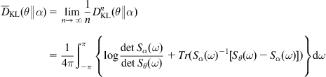 (5.27)
Theorem 5.3
![]() , with equality if and only if
, with equality if and only if ![]() ,
, ![]() .
.
Proof:
![]() , the spectral density matrices
, the spectral density matrices ![]() and
and ![]() are positive definite. Let
are positive definite. Let ![]() and
and ![]() be two normally distributed
be two normally distributed ![]() -dimensional vectors,
-dimensional vectors, ![]() and
and ![]() , respectively. Then we have
, respectively. Then we have
![]() (5.28)
(5.28)
Combining Eqs. (5.28) and (5.27) yields
![]() (5.29)
(5.29)
It follows easily that ![]() , with equality if and only if
, with equality if and only if ![]() for almost every
for almost every ![]() (hence
(hence ![]() ,
, ![]() ).
).
By Theorem 5.3, we may conclude that for a stationary Gaussian process, ![]() is KLIDR-identifiable if and only if
is KLIDR-identifiable if and only if ![]() ,
, ![]() implies
implies ![]() . This is exactly the identifiability from the output spectral density.
. This is exactly the identifiability from the output spectral density.
5.1.4 Markov Process Case
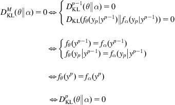
Now we focus on situations where the observation sequence is a parameterized Markov process. First, let us define the minimum identifiable horizon (MIH).
Definition 5.4
Assume that ![]() is KLID-identifiable. Then the MIH is [120]:
is KLID-identifiable. Then the MIH is [120]:
![]() (5.30)
(5.30)
where ![]() .
.
The MIH is the minimum length of the observation sequence from which ![]() can be uniquely identified. If the MIH is known, we could identify
can be uniquely identified. If the MIH is known, we could identify ![]() with the least observation data. In general, it is difficult to obtain the exact value of MIH. In some special situations, however, one can derive an upper bound on the MIH. For a parameterized Markov process, this upper bound is straightforward. In the theorem below, we show that for a
with the least observation data. In general, it is difficult to obtain the exact value of MIH. In some special situations, however, one can derive an upper bound on the MIH. For a parameterized Markov process, this upper bound is straightforward. In the theorem below, we show that for a ![]() -order strictly stationary Markov process, the number
-order strictly stationary Markov process, the number ![]() provides an upper bound on the MIH.
provides an upper bound on the MIH.
Theorem 5.4
If the observation sequence ![]() (
(![]() ) is a
) is a ![]() -order strictly stationary Markov process (
-order strictly stationary Markov process (![]() ), and the parameter set
), and the parameter set ![]() is KLID-identifiable at
is KLID-identifiable at ![]() , then we have
, then we have ![]() .
.
Proof:
As parameter set ![]() is KLID-identifiable at
is KLID-identifiable at ![]() , by Definition 5.1, there exists a number
, by Definition 5.1, there exists a number ![]() , such that
, such that ![]() ,
, ![]() . Let us consider two cases, one for which
. Let us consider two cases, one for which ![]() and the other for which
and the other for which ![]() .
.
1. ![]() : The zero-order strictly stationary Markov process refers to an independent and identically distributed sequence. In this case, we have
: The zero-order strictly stationary Markov process refers to an independent and identically distributed sequence. In this case, we have ![]() , and
, and
 (5.31)
And hence, ![]() , we have
, we have ![]() . It follows that
. It follows that ![]() , and
, and ![]() .
.
![]() (5.32)
(5.32)
By Markovian and stationary properties, one can derive
 (5.33)
 (5.34)
where ![]() is the conditional KLID. And hence,
is the conditional KLID. And hence,
 (5.35)
Example 5.2
Consider the first-order AR model (![]() ) [120]:
) [120]:
![]() (5.36)
(5.36)
where ![]() is a zero-mean white Gaussian noise with unit power. Assume that the system has reached steady state when the observations begin. The observation sequence
is a zero-mean white Gaussian noise with unit power. Assume that the system has reached steady state when the observations begin. The observation sequence ![]() will be a first-order stationary Gaussian Markov process, with covariance matrix:
will be a first-order stationary Gaussian Markov process, with covariance matrix:
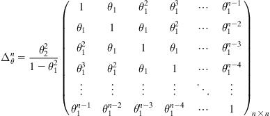 (5.37)
![]() (
(![]() ,
, ![]() ), we have
), we have
![]() (5.38)
(5.38)
where ![]() are the RCVs. And hence,
are the RCVs. And hence, ![]() .
.
The following corollary is a direct consequence of Theorem 5.4.
Corollary 5.1
For a ![]() -order strictly stationary Markov process
-order strictly stationary Markov process ![]() , the parameter set
, the parameter set ![]() is KLID-identifiable at
is KLID-identifiable at ![]() if and only if
if and only if ![]() ,
, ![]() implies
implies ![]() .
.
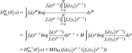
From the theory of stochastic process, for a ![]() -order strictly stationary Markov process
-order strictly stationary Markov process ![]() , under certain conditions (see Ref. [221] for details), the conditional density
, under certain conditions (see Ref. [221] for details), the conditional density ![]() will determine uniquely the joint density
will determine uniquely the joint density ![]() . In this case, the KLID-identifiability and the KLIDR-identifiability are equivalent.
. In this case, the KLID-identifiability and the KLIDR-identifiability are equivalent.
Theorem 5.5
Assume that the observation sequence ![]() is a
is a ![]() -order strictly stationary Markov process (
-order strictly stationary Markov process (![]() ), whose conditional density
), whose conditional density ![]() uniquely determines the joint density
uniquely determines the joint density ![]() . Then,
. Then, ![]() ,
, ![]() is KLID-identifiable if and only if it is KLIDR-identifiable.
is KLID-identifiable if and only if it is KLIDR-identifiable.


5.1.5 Asymptotic KLID-Identifiability
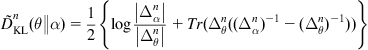
In the previous discussions, we assume that the true density ![]() is known. In most practical situations, however, the actual density, and hence the KLID, needs to be estimated using random data drawn from the underlying density. Let
is known. In most practical situations, however, the actual density, and hence the KLID, needs to be estimated using random data drawn from the underlying density. Let ![]() be an independent and identically distributed (i.i.d.) sample drawn from
be an independent and identically distributed (i.i.d.) sample drawn from ![]() . The density estimator for
. The density estimator for ![]() will be a mapping
will be a mapping ![]() [98]:
[98]:
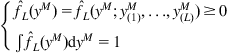 (5.41)
The asymptotic KLID-identifiability is then defined as follows:
Definition 5.5
The parameter set ![]() is said to be asymptotic KLID-identifiable at
is said to be asymptotic KLID-identifiable at ![]() , if there exists a sequence of density estimates
, if there exists a sequence of density estimates ![]() , such that
, such that ![]() (convergence in probability), where
(convergence in probability), where ![]() is the minimum KLID estimator,
is the minimum KLID estimator, ![]() .
.
Theorem 5.6
Assume that the parameter space ![]() is a compact subset, and the density estimate sequence
is a compact subset, and the density estimate sequence ![]() satisfies
satisfies ![]() . Then,
. Then, ![]() will be asymptotic KLID-identifiable provided it is KLID-identifiable.
will be asymptotic KLID-identifiable provided it is KLID-identifiable.
Proof:
Since ![]() , for
, for ![]() and
and ![]() arbitrarily small, there exists an
arbitrarily small, there exists an ![]() such that for
such that for ![]() ,
,
![]() (5.42)
(5.42)
where ![]() is the probability of Borel set
is the probability of Borel set ![]() . On the other hand, as
. On the other hand, as ![]() , we have
, we have
![]() (5.43)
(5.43)
Then the event ![]() , and hence
, and hence
![]() (5.44)
(5.44)
By Pinsker’s inequality, we have
 (5.45)
where ![]() is the
is the ![]() -distance (or the total variation). It follows that
-distance (or the total variation). It follows that
 (5.46)
In addition, the following inequality holds:
![]() (5.47)
(5.47)
Then we have
![]() (5.48)
(5.48)
And hence
 (5.49)
For any ![]() , we define the set
, we define the set ![]() , where
, where ![]() is the Euclidean norm. As
is the Euclidean norm. As ![]() is a compact subset in
is a compact subset in ![]() ,
, ![]() must be a compact set too. Meanwhile, by Assumption 5.2, the function
must be a compact set too. Meanwhile, by Assumption 5.2, the function ![]() (
(![]() ) will be a continuous mapping
) will be a continuous mapping ![]() . Thus, a minimum of
. Thus, a minimum of ![]() over the set
over the set ![]() must exist. Denote
must exist. Denote ![]() , it follows easily that
, it follows easily that
![]() (5.50)
(5.50)
If ![]() is KLID-identifiable,
is KLID-identifiable, ![]() ,
, ![]() , we have
, we have ![]() , or equivalently,
, or equivalently, ![]() . It follows that
. It follows that ![]() . Let
. Let ![]() , we have
, we have
 (5.51)
This implies ![]() , and hence
, and hence ![]() .
.
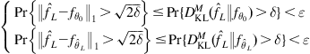
According to Theorem 5.6, if the density estimate ![]() is consistent in KLID in probability (
is consistent in KLID in probability (![]() ), the KLID-identifiability will be a sufficient condition for the asymptotic KLID-identifiability. The next theorem shows that, under certain conditions, the KLID-identifiability will also be a necessary condition for
), the KLID-identifiability will be a sufficient condition for the asymptotic KLID-identifiability. The next theorem shows that, under certain conditions, the KLID-identifiability will also be a necessary condition for ![]() to be asymptotic KLID-identifiable.
to be asymptotic KLID-identifiable.
Theorem 5.7
If ![]() is asymptotic KLID-identifiable, then it is KLID-identifiable provided
is asymptotic KLID-identifiable, then it is KLID-identifiable provided
Proof:
If ![]() is asymptotic KLID-identifiable, then for
is asymptotic KLID-identifiable, then for ![]() and
and ![]() arbitrarily small, there exists an
arbitrarily small, there exists an ![]() such that for
such that for ![]() ,
,
![]() (5.53)
(5.53)
Suppose ![]() is not KLID-identifiable, then
is not KLID-identifiable, then ![]() ,
, ![]() , such that
, such that ![]() . Let
. Let ![]() , we have (as
, we have (as ![]() is a compact subset, the minimum exists)
is a compact subset, the minimum exists)
 (5.54)
where (a) follows from ![]() . The above result contradicts the condition (2). Therefore,
. The above result contradicts the condition (2). Therefore, ![]() must be KLID-identifiable.
must be KLID-identifiable.
In the following, we consider several specific density estimation methods and discuss the consistency problems of the related parameter estimators.
5.1.5.1 Maximum Likelihood Estimation
The maximum likelihood estimation (MLE) is a popular parameter estimation method and is also an important parametric approach for the density estimation. By MLE, the density estimator is
![]() (5.55)
(5.55)
where ![]() is obtained by maximizing the likelihood function, that is,
is obtained by maximizing the likelihood function, that is,
![]() (5.56)
(5.56)
Lemma 5.1
The MLE density estimate sequence ![]() satisfies
satisfies ![]() .
.
A simple proof of this lemma can be found in Ref. [222]. Combining Theorem 5.6 and Lemma 5.1, we have the following corollary.
Corollary 5.2
Assume that ![]() is a compact subset in
is a compact subset in ![]() , and
, and ![]() is KLID-identifiable. Then we have
is KLID-identifiable. Then we have ![]() .
.
According to Corollary 5.2, the KLID-identifiability is a sufficient condition to guarantee the ML estimator to converge to the true value in probability one. This is not surprising since the ML estimator is in essence a special case of the minimum KLID estimator.
5.1.5.2 Histogram-Based Estimation
The histogram-based estimation is a common nonparametric method for density estimation. Suppose the i.i.d. samples ![]() take values in a measurable space
take values in a measurable space ![]() . Let
. Let ![]() ,
, ![]() , be a sequence of partitions of
, be a sequence of partitions of ![]() , with
, with ![]() either finite or infinite, such that the
either finite or infinite, such that the ![]() -measure
-measure ![]() for each
for each ![]() . Then the standard histogram density estimator with respect to
. Then the standard histogram density estimator with respect to ![]() and
and ![]() is given by:
is given by:
![]() (5.57)
(5.57)
where ![]() is the standard empirical measure of
is the standard empirical measure of ![]() , i.e.,
, i.e.,
![]() (5.58)
(5.58)
where ![]() is the indicator function.
is the indicator function.
According to Ref. [223], under certain conditions, the density estimator ![]() will converge in reversed order information divergence to the true underlying density
will converge in reversed order information divergence to the true underlying density ![]() , and the expected KLID
, and the expected KLID
![]() (5.59)
(5.59)
Since ![]() , by Markov’s inequality [224], for any
, by Markov’s inequality [224], for any ![]() , we have
, we have
![]() (5.60)
(5.60)
It follows that ![]() ,
, ![]() , and for any
, and for any ![]() and
and ![]() arbitrarily small, there exists an
arbitrarily small, there exists an ![]() such that for
such that for ![]() ,
,
![]() (5.61)
(5.61)
Thus we have ![]() . By Theorem 5.6, the following corollary holds.
. By Theorem 5.6, the following corollary holds.
Corollary 5.3
Assume that ![]() is a compact subset in
is a compact subset in ![]() , and
, and ![]() is KLID-identifiable. Let
is KLID-identifiable. Let ![]() be the standard histogram density estimator satisfying Eq. (5.59). Then we have
be the standard histogram density estimator satisfying Eq. (5.59). Then we have ![]() , where
, where ![]() .
.
5.1.5.3 Kernel-Based Estimation
The kernel-based estimation (or kernel density estimation, KDE) is another important nonparametric approach for the density estimation. Given an i.i.d. sample ![]() , the kernel density estimator is
, the kernel density estimator is
 (5.62)
where ![]() is a kernel function satisfying
is a kernel function satisfying ![]() and
and ![]() ,
, ![]() is the kernel width.
is the kernel width.
For the KDE, the following lemma holds (see chapter 9 in Ref. [98] for details).
Lemma 5.2
Assume that ![]() is a fixed kernel, and the kernel width
is a fixed kernel, and the kernel width ![]() depends on
depends on ![]() only. If
only. If ![]() and
and ![]() as
as ![]() , then
, then ![]() .
.
From ![]() , one cannot derive
, one cannot derive ![]() . And hence, Theorem 5.6 cannot be applied here. However, if the parameter is estimated by minimizing the total variation (not the KLID), the following theorem holds.
. And hence, Theorem 5.6 cannot be applied here. However, if the parameter is estimated by minimizing the total variation (not the KLID), the following theorem holds.
Theorem 5.8
Assume that ![]() is a compact subset in
is a compact subset in ![]() ,
, ![]() is KLID-identifiable, and the kernel width
is KLID-identifiable, and the kernel width ![]() satisfies the conditions in Lemma 5.2. Then we have
satisfies the conditions in Lemma 5.2. Then we have ![]() , where
, where ![]() .
.
Proof:
As ![]() , by Markov’s inequality, we have
, by Markov’s inequality, we have ![]() . Following a similar derivation as for Theorem 5.6, one can easily reach the conclusion.
. Following a similar derivation as for Theorem 5.6, one can easily reach the conclusion.
The KLID and the total variation are both special cases of the family of ![]() -divergence [130]. The
-divergence [130]. The ![]() -divergence between the PDFs
-divergence between the PDFs ![]() and
and ![]() is
is
![]() (5.63)
(5.63)
where ![]() is a class of convex functions. The minimum
is a class of convex functions. The minimum ![]() -divergence estimator is given by [130]:
-divergence estimator is given by [130]:
![]() (5.64)
(5.64)
Below we give a more general result, which includes Theorems 5.6 and 5.8 as special cases.
Theorem 5.9
Assume that ![]() is a compact subset in
is a compact subset in ![]() ,
, ![]() is KLID-identifiable, and for a given
is KLID-identifiable, and for a given ![]() ,
, ![]() ,
, ![]() , where function
, where function ![]() is strictly increasing over the interval
is strictly increasing over the interval ![]() , and
, and ![]() . Then, if the density estimate sequence
. Then, if the density estimate sequence ![]() satisfies
satisfies ![]() , we have
, we have ![]() , where
, where ![]() is the minimum
is the minimum ![]() -divergence estimator.
-divergence estimator.
5.2 Minimum Information Divergence Identification with Reference PDF
Information divergences have been suggested by many authors for the solution of the related problems of system identification. The ML criterion and its extensions (e.g., AIC) can be derived from the KL divergence approach. The information divergence approach is a natural generalization of the LS view. Actually one can think of a “distance” between the actual (empirical) and model distributions of the data, without necessarily introducing the conceptually more demanding concepts of likelihood or posterior. In the following, we introduce a novel system identification approach based on the minimum information divergence criterion.
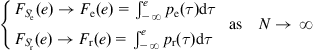
Apart from conventional methods, the new approach adopts the idea of PDF shaping and uses the divergence between the actual error PDF and a reference (or target) PDF (usually with zero mean and a narrow range) as the identification criterion. As illustrated in Figure 5.1, in this scheme, the model parameters are adjusted such that the error distribution tends to the reference distribution. With KLID, the optimal parameters (or weights) of the model can be expressed as:
![]() (5.65)
(5.65)
where ![]() and
and ![]() denote, respectively, the actual error PDF and the reference PDF. Other information divergence measures such as
denote, respectively, the actual error PDF and the reference PDF. Other information divergence measures such as ![]() -divergence can also be used but are not considered here.
-divergence can also be used but are not considered here.

The above method shapes the error distribution, and can be used to achieve the desired variance or entropy of the error, provided the desired PDF of the error can be achieved. This is expected to be useful in complex signal processing and learning systems. If we choose the ![]() function as the reference PDF, the identification error will be forced to concentrate around the zero with a sharper peak. This coincides with commonsense predictions about system identification.
function as the reference PDF, the identification error will be forced to concentrate around the zero with a sharper peak. This coincides with commonsense predictions about system identification.
It is worth noting that the PDF shaping approaches can be found in other contexts. In the control literature, Karny et al. [225,226] proposed an alternative formulation of stochastic control design problem: the joint distributions of closed-loop variables should be forced to be as close as possible to their desired distributions. This formulation is called the fully probabilistic control. Wang et al. [227–229] designed new algorithms to control the shape of the output PDF of a stochastic dynamic system. In adaptive signal processing literature, Sala-Alvarez et al. [230] proposed a general criterion for the design of adaptive systems in digital communications, called the statistical reference criterion, which imposes a given PDF at the output of an adaptive system.
It is important to remark that the minimum value of the KLID in Eq. (5.65) may not be zero. In fact, all the possible PDFs of the error are, in general, restricted to a certain set of functions ![]() . If the reference PDF is not contained in the possible PDF set, i.e.,
. If the reference PDF is not contained in the possible PDF set, i.e., ![]() , we have
, we have
![]() (5.66)
(5.66)
In this case, the optimal error PDF ![]() , and the reference distribution can never be realized. This is however not a problem of great concern, since our goal is just to make the error distribution closer (not necessarily identical) to the reference distribution.
, and the reference distribution can never be realized. This is however not a problem of great concern, since our goal is just to make the error distribution closer (not necessarily identical) to the reference distribution.
In some special situations, this new identification method is equivalent to the ML identification. Suppose that in Figure 5.1 the noise ![]() is independent of the input
is independent of the input ![]() , and the unknown system can be exactly identified, i.e., the intrinsic error (
, and the unknown system can be exactly identified, i.e., the intrinsic error (![]() ) between the unknown system and the model can be zero. In addition, we assume that the noise PDF
) between the unknown system and the model can be zero. In addition, we assume that the noise PDF ![]() is known. In this case, if setting
is known. In this case, if setting ![]() , we have
, we have
 (5.67)
where (a) comes from the fact that the weight vector minimizing the KLID (when ![]() ) also minimizes the error entropy, and
) also minimizes the error entropy, and ![]() is the likelihood function.
is the likelihood function.
5.2.1 Some Properties
We present in the following some important properties of the minimum KLID criterion with reference PDF (called the KLID criterion for short).
The KLID criterion is much different from the minimum error entropy (MEE) criterion. The MEE criterion does not consider the mean of the error due to its invariance to translation. Under MEE criterion, the estimator makes the error PDF as sharp as possible, and neglects the PDF’s location. Under KLID criterion, however, the estimator makes the actual error PDF and reference PDF as close as possible (in both shape and location).
The KLID criterion is sensitive to the error mean. This can be easily verified: if ![]() and
and ![]() are both Gaussian PDFs with zero mean and unit variance, we have
are both Gaussian PDFs with zero mean and unit variance, we have ![]() ; while if the error mean becomes nonzero,
; while if the error mean becomes nonzero, ![]() , we have
, we have ![]() . The following theorem suggests that, under certain conditions the mean value of the optimal error PDF under KLID criterion is equal to the mean value of the reference PDF.
. The following theorem suggests that, under certain conditions the mean value of the optimal error PDF under KLID criterion is equal to the mean value of the reference PDF.
Theorem 5.10
Assume that ![]() and
and ![]() satisfy:
satisfy:
2. ![]() ,
, ![]() is an even function, where
is an even function, where ![]() is the mean value of
is the mean value of ![]() ;
;
3. ![]() is an even and strictly log-concave function, where
is an even and strictly log-concave function, where ![]() is the mean value of
is the mean value of ![]() .
.
Then, the mean value of the optimal error PDF (![]() ) is
) is ![]() .
.
Proof:
Using reduction to absurdity. Suppose ![]() , and let
, and let ![]() . Denote
. Denote ![]() and
and ![]() . According to the assumptions,
. According to the assumptions, ![]() , and
, and ![]() is an even function. Then we have
is an even function. Then we have
 (5.68)
where (a), (d), and (e) follow from the shift-invariance of the KLID, (b) is because ![]() is strictly log-concave, and (c) is because
is strictly log-concave, and (c) is because ![]() and
and ![]() are even functions. Therefore,
are even functions. Therefore, ![]() , such that
, such that
![]() (5.69)
(5.69)
This contradicts with ![]() . And hence,
. And hence, ![]() holds.
holds.
On the other hand, the KLID criterion is also closely related to the MEE criterion. The next theorem provides an upper bound on the error entropy under the constraint that the KLID is bounded.
Theorem 5.11
Let the reference PDF ![]() be a zero-mean Gaussian PDF with variance
be a zero-mean Gaussian PDF with variance ![]() . If the error PDF
. If the error PDF ![]() satisfies
satisfies
![]() (5.70)
(5.70)
where ![]() is a positive constant, then the error entropy
is a positive constant, then the error entropy ![]() satisfies
satisfies
![]() (5.71)
(5.71)
where ![]() is the solution of the following equation:
is the solution of the following equation:
![]() (5.72)
(5.72)
Proof:
Denote ![]() the collection of all the error PDFs that satisfy
the collection of all the error PDFs that satisfy ![]() . Clearly, this is a convex set.
. Clearly, this is a convex set. ![]() , we have
, we have
![]() (5.73)
(5.73)
In order to solve the error distribution that achieves the maximum entropy, we create the Lagrangian:
![]() (5.74)
(5.74)
where ![]() and
and ![]() are the Lagrange multipliers. When
are the Lagrange multipliers. When ![]() ,
, ![]() is a concave function of
is a concave function of ![]() . If
. If ![]() is a function such that
is a function such that ![]() for
for ![]() sufficiently small, the Gateaux derivative of
sufficiently small, the Gateaux derivative of ![]() with respect to
with respect to ![]() is given by:
is given by:
 (5.75)
If it is zero for all ![]() , we have
, we have
![]() (5.76)
(5.76)
Thus, if ![]() (such that
(such that ![]() is a concave function of
is a concave function of ![]() ), the error PDF that achieves the maximum entropy exists and is given by
), the error PDF that achieves the maximum entropy exists and is given by
![]() (5.77)
(5.77)
According to the assumptions, ![]() . It follows that
. It follows that
![]() (5.78)
(5.78)
where ![]() . Obviously,
. Obviously, ![]() is a Gaussian density, and we have
is a Gaussian density, and we have
![]() (5.79)
(5.79)
So ![]() can be determined as
can be determined as
 (5.80)
In order to determine the value of ![]() , we use the Kuhn–Tucker condition:
, we use the Kuhn–Tucker condition:
![]() (5.81)
(5.81)
When ![]() , we have
, we have ![]() , that is,
, that is,
![]() (5.82)
(5.82)
Therefore, ![]() is the solution of the Eq. (5.72).
is the solution of the Eq. (5.72).
Define the function ![]() . It is easy to verify that
. It is easy to verify that ![]() is continuous and monotonically decreasing over interval
is continuous and monotonically decreasing over interval ![]() . Since
. Since ![]() ,
, ![]() , and
, and ![]() , the equation
, the equation ![]() certainly has a solution in
certainly has a solution in ![]() .
.
From the previous derivations, one may easily obtain:
![]() (5.83)
(5.83)
The above theorem indicates that, under the KLID constraint ![]() , the error entropy is upper bounded by the reference entropy plus a certain constant. In particular, when
, the error entropy is upper bounded by the reference entropy plus a certain constant. In particular, when ![]() , we have
, we have ![]() and
and ![]() . Therefore, if one chooses a reference PDF with small entropy, the error entropy will also be confined within small values. In practice, the reference PDF is, in general, chosen as a PDF with zero mean and small entropy (e.g., the
. Therefore, if one chooses a reference PDF with small entropy, the error entropy will also be confined within small values. In practice, the reference PDF is, in general, chosen as a PDF with zero mean and small entropy (e.g., the ![]() distribution at zero).
distribution at zero).
In most practical situations, the error PDF is unknown and needs to be estimated from samples. There is always a bias in the density estimation; in order to offset the influence of the bias, one can use the same method to estimate the reference density based on the samples drawn from the reference PDF. Let ![]() and
and ![]() be respectively the actual and reference error samples. The KDEs of
be respectively the actual and reference error samples. The KDEs of ![]() and
and ![]() will be
will be
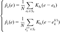 (5.84)
where ![]() and
and ![]() are corresponding kernel widths. Using the estimated PDFs, one may obtain the empirical KLID criterion
are corresponding kernel widths. Using the estimated PDFs, one may obtain the empirical KLID criterion ![]() .
.
Theorem 5.12
The empirical KLID ![]() , with equality if and only if
, with equality if and only if ![]() .
.
Proof:
![]() , we have
, we have ![]() , with equality if and only if
, with equality if and only if ![]() . And hence
. And hence
 (5.85)
with equality if and only if ![]() .
.
Theorem 5.13
If ![]() is a Gaussian kernel function,
is a Gaussian kernel function, ![]() , then
, then
![]() (5.87)
(5.87)
Proof:
Since Gaussian kernel is bounded, and ![]() , the kernel-based density estimates
, the kernel-based density estimates ![]() and
and ![]() will also be bounded, and
will also be bounded, and
 (5.88)
By Lemma 5.3, we have
![]() (5.89)
(5.89)
where
 (5.90)
Then we obtain Eq. (5.87).
The above theorem suggests that convergence in KLID ensures the convergence in ![]() distance (
distance ( ).
).
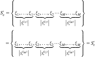
Before giving Theorem 5.14, we introduce some notations. By rearranging the samples in ![]() and
and ![]() , one obtains the increasing sequences:
, one obtains the increasing sequences:
 (5.91)
where ![]() ,
, ![]() . Denote
. Denote ![]() , and
, and ![]() .
.
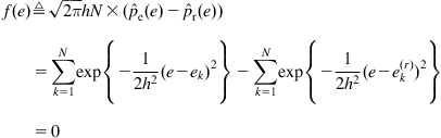
Theorem 5.14
If ![]() is a Gaussian kernel function,
is a Gaussian kernel function, ![]() , then
, then ![]() if and only if
if and only if ![]() .
.
Proof:
By Theorem 5.12, it suffices to prove that ![]() if and only if
if and only if ![]() .
.
Sufficiency: If ![]() , we have
, we have
 (5.92)
Necessity: If ![]() , then we have
, then we have
 (5.93)
Let ![]() , where
, where ![]() . Then,
. Then,
![]() (5.94)
(5.94)
where ![]() ,
, ![]() ,
, ![]() . Since
. Since ![]() ,
, ![]() , we have
, we have ![]() . It follows that
. It follows that
 (5.95)
As ![]() is a symmetric and positive definite matrix (
is a symmetric and positive definite matrix (![]() ), we get
), we get ![]() , that is
, that is
![]() (5.96)
(5.96)
Thus, ![]() , and
, and
 (5.97)
This completes the proof.
Theorem 5.14 indicates that, under certain conditions the zero value of the empirical KLID occurs only when the actual and reference sample sets are identical.
Based on the sample sets ![]() and
and ![]() , one can calculate the empirical distribution:
, one can calculate the empirical distribution:
![]() (5.98)
(5.98)
where ![]() , and
, and ![]() . According to the limit theorem in probability theory [224], we have
. According to the limit theorem in probability theory [224], we have
 (5.99)
If ![]() , and
, and ![]() is large enough, we have
is large enough, we have ![]() , and hence
, and hence ![]() . Therefore, when the empirical KLID approaches zero, the actual error PDF will be approximately identical with the reference PDF.
. Therefore, when the empirical KLID approaches zero, the actual error PDF will be approximately identical with the reference PDF.
5.2.2 Identification Algorithm
In the following, we derive a stochastic gradient–based identification algorithm under the minimum KLID criterion with a reference PDF. Since the KLID is not symmetric, we use the symmetric version of KLID (also referred to as the J-information divergence):
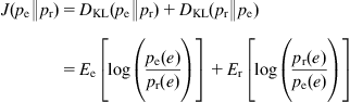 (5.100)
By dropping off the expectation operators ![]() and
and ![]() , and plugging in the estimated PDFs, one may obtain the estimated instantaneous value of J-information divergence:
, and plugging in the estimated PDFs, one may obtain the estimated instantaneous value of J-information divergence:
![]() (5.101)
(5.101)
where ![]() and
and ![]() are
are
 (5.102)
Then a stochastic gradient–based algorithm can be readily derived as follows:
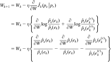 (5.103)
where
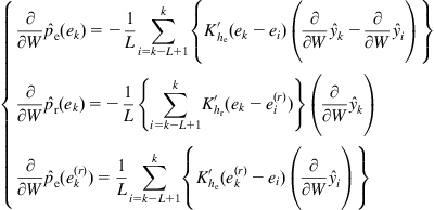 (5.104)
This algorithm is called the stochastic information divergence gradient (SIDG) algorithm [125,126].
In order to achieve an error distribution with zero mean and small entropy, one can choose the ![]() function at zero as the reference PDF. It is, however, worth noting that the
function at zero as the reference PDF. It is, however, worth noting that the ![]() function is not always the best choice. In many situations, the desired error distribution may be far from the
function is not always the best choice. In many situations, the desired error distribution may be far from the ![]() distribution. In practice, the desired error distribution can be estimated from some prior knowledge or preliminary identification results.
distribution. In practice, the desired error distribution can be estimated from some prior knowledge or preliminary identification results.
Remark:
Strictly speaking, if one selects the ![]() function as the reference distribution, the information divergence will be undefined (ill-posed). In practical applications, however, we often use the estimated information divergence as an alternative cost function, where the actual and reference error distributions are both estimated by KDE approach (usually with the same kernel width). It is easy to verify that, for the
function as the reference distribution, the information divergence will be undefined (ill-posed). In practical applications, however, we often use the estimated information divergence as an alternative cost function, where the actual and reference error distributions are both estimated by KDE approach (usually with the same kernel width). It is easy to verify that, for the ![]() distribution, the estimated PDF is actually the kernel function. In this case, the estimated divergence will always be valid.
distribution, the estimated PDF is actually the kernel function. In this case, the estimated divergence will always be valid.
5.2.3 Simulation Examples
Example 5.3
Consider the FIR system identification [126]:
![]() (5.105)
(5.105)
where the true weight vector ![]() . The input signal
. The input signal ![]() is assumed to be a zero-mean white Gaussian process with unit power.
is assumed to be a zero-mean white Gaussian process with unit power.
We show that the optimal solution under information divergence criterion may be not unique. Suppose the reference PDF ![]() is Gaussian PDF with zero mean and variance
is Gaussian PDF with zero mean and variance ![]() . The J-information divergence between
. The J-information divergence between ![]() and
and ![]() can be calculated as:
can be calculated as:
![]() (5.106)
(5.106)
Clearly, there are infinitely many weight pairs ![]() that satisfy
that satisfy ![]() . In fact, any weight pair
. In fact, any weight pair ![]() that lies on the circle
that lies on the circle ![]() will be an optimal solution. In this case, the system parameters are not identifiable. However, when
will be an optimal solution. In this case, the system parameters are not identifiable. However, when ![]() , the circle will shrink to a point and all the solutions will converge to a unique solution
, the circle will shrink to a point and all the solutions will converge to a unique solution ![]() . For the case
. For the case ![]() , the 3D surface of the J-information divergence is depicted in Figure 5.2. Figure 5.3 draws the convergence trajectories of the weight pair
, the 3D surface of the J-information divergence is depicted in Figure 5.2. Figure 5.3 draws the convergence trajectories of the weight pair ![]() learned by the SIDG algorithm, starting from the initial point
learned by the SIDG algorithm, starting from the initial point ![]() . As expected, these trajectories converge to the circles centered at
. As expected, these trajectories converge to the circles centered at ![]() . When
. When ![]() , the weight pair
, the weight pair ![]() will converge to (1.0047, 0.4888), which is very close to the true weight vector.
will converge to (1.0047, 0.4888), which is very close to the true weight vector.

Figure 5.2 3D surface of J-information divergence. Source: Adapted from Ref. [126].
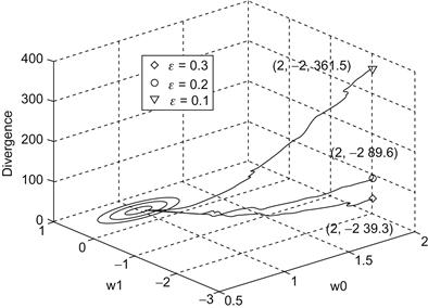
Figure 5.3 Convergence trajectories of weight pair (![]() ,
,![]() ). Source: Adapted from Ref. [126].
). Source: Adapted from Ref. [126].
Example 5.4
Identification of the hybrid system (switch system) [125]:
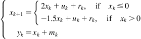 (5.107)
where ![]() is the state variable,
is the state variable, ![]() is the input,
is the input, ![]() is the process noise, and
is the process noise, and ![]() is the measurement noise. This system can be written in a parameterized form (
is the measurement noise. This system can be written in a parameterized form (![]() merging into
merging into ![]() ) [125]:
) [125]:
![]() (5.108)
(5.108)
where ![]() is the mode index,
is the mode index, ![]() ,
, ![]() ,
, ![]() , and
, and ![]() . In this example,
. In this example, ![]() and
and ![]() . Based on the parameterized form (Eq. (5.108)), one can establish the noisy hybrid decoupling polynomial (NHDP) [125]. By expanding the NHDP and ignoring the higher-order components of the noise, we obtain the first-order approximation (FOA) model. In Ref. [125], the SIDG algorithm (based on the FOA model) was applied to identify the above hybrid system. Figure 5.4 shows the identification performance for different measurement noise powers
. Based on the parameterized form (Eq. (5.108)), one can establish the noisy hybrid decoupling polynomial (NHDP) [125]. By expanding the NHDP and ignoring the higher-order components of the noise, we obtain the first-order approximation (FOA) model. In Ref. [125], the SIDG algorithm (based on the FOA model) was applied to identify the above hybrid system. Figure 5.4 shows the identification performance for different measurement noise powers ![]() . For comparison purpose, we also draw the performance of the least mean square (LMS) and algebraic geometric approach [232]. In Figure 5.4, the identification performance
. For comparison purpose, we also draw the performance of the least mean square (LMS) and algebraic geometric approach [232]. In Figure 5.4, the identification performance ![]() is defined as:
is defined as:
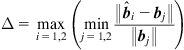 (5.109)
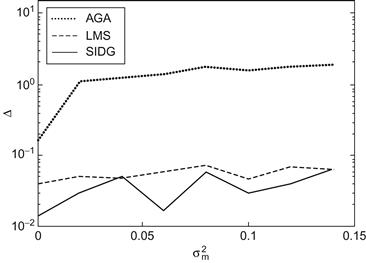
Figure 5.4 Identification performance for different measurement noise powers. Source: Adapted from Ref. [125].
In the simulation, the ![]() function is selected as the reference PDF for SIDG algorithm. Simulation results indicate that the SIDG algorithm can achieve a better performance.
function is selected as the reference PDF for SIDG algorithm. Simulation results indicate that the SIDG algorithm can achieve a better performance.
To further verify the performance of the SIDG algorithm, we consider the case in which ![]() and
and ![]() is uniformly distributed in the range of
is uniformly distributed in the range of ![]() . The reference samples are set to
. The reference samples are set to ![]() according to some preliminary identification results. Figure 5.5 shows the scatter graphs of the estimated parameter vector
according to some preliminary identification results. Figure 5.5 shows the scatter graphs of the estimated parameter vector ![]() (with 300 simulation runs), where (A) and (B) correspond, respectively, to the LMS and SIDG algorithms. In each graph, there are two clusters. Evidently, the clusters generated by SIDG are more compact than those generated by LMS, and the centers of the former are closer to the true values than those of the latter (the true values are
(with 300 simulation runs), where (A) and (B) correspond, respectively, to the LMS and SIDG algorithms. In each graph, there are two clusters. Evidently, the clusters generated by SIDG are more compact than those generated by LMS, and the centers of the former are closer to the true values than those of the latter (the true values are ![]() and
and ![]() ). The involved error PDFs are illustrated in Figure 5.6. As one can see, the error distribution produced by SIDG is closer to the desired error distribution.
). The involved error PDFs are illustrated in Figure 5.6. As one can see, the error distribution produced by SIDG is closer to the desired error distribution.


Figure 5.6 Comparison of the error PDFs. Source: Adapted from Ref. [125].
5.2.4 Adaptive Infinite Impulsive Response Filter with Euclidean Distance Criterion
In Ref. [233], the Euclidean distance criterion (EDC), which can be regarded as a special case of the information divergence criterion with a reference PDF, was successfully applied to develop the global optimization algorithms for adaptive infinite impulsive response (IIR) filters. In the following, we give a brief introduction of this approach.
The EDC for the adaptive IIR filters is defined as the Euclidean distance (or L2 distance) between the error PDF and ![]() function [233]:
function [233]:
![]() (5.110)
(5.110)
The above formula can be expanded as:
![]() (5.111)
(5.111)
where ![]() stands for the parts of this Euclidean distance measure that do not depend on the error distribution. By dropping
stands for the parts of this Euclidean distance measure that do not depend on the error distribution. By dropping ![]() , the EDC can be simplified to
, the EDC can be simplified to
![]() (5.112)
(5.112)
where ![]() is the quadratic information potential of the error.
is the quadratic information potential of the error.
By substituting the kernel density estimator (usually with Gaussian kernel ![]() ) for the error PDF in the integral, one may obtain the empirical EDC:
) for the error PDF in the integral, one may obtain the empirical EDC:
 (5.113)
A gradient-based identification algorithm can then be derived as follows:
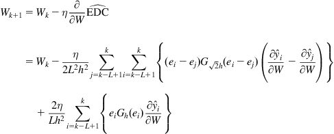 (5.114)
where the gradient ![]() depends on the model structure. Below we derive this gradient for the IIR filters.
depends on the model structure. Below we derive this gradient for the IIR filters.
Let us consider the following IIR filter:
![]() (5.115)
(5.115)
which can be written in the form
![]() (5.116)
(5.116)
where ![]() ,
, ![]() . Then we can derive
. Then we can derive
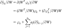 (5.117)
In Eq. (5.117), the parameter gradient is calculated in a recursive manner.
Example 5.5
Identifying the following unknown system [233]:
![]() (5.118)
(5.118)
The adaptive model is chosen to be the reduced order IIR filter
![]() (5.119)
(5.119)
The main goal is to determine the values of the coefficients (or weights) ![]() , such that the EDC is minimized. Assume that the error is Gaussian distributed,
, such that the EDC is minimized. Assume that the error is Gaussian distributed, ![]() . Then, the empirical EDC can be approximately calculated as [233]:
. Then, the empirical EDC can be approximately calculated as [233]:
![]() (5.120)
(5.120)
where ![]() is the kernel width. Figure 5.7 shows the contours of the EDC performance surface in different
is the kernel width. Figure 5.7 shows the contours of the EDC performance surface in different ![]() (the input signal is assumed to be a white Gaussian noise with zero mean and unit variance). As one can see, the local minima of the performance surface have disappeared with large kernel width. Thus, by carefully controlling the kernel width, the algorithm can converge to the global minimum. The convergence trajectory of the adaptation process with the weight approaching to the global minimum is shown in Figure 5.8.
(the input signal is assumed to be a white Gaussian noise with zero mean and unit variance). As one can see, the local minima of the performance surface have disappeared with large kernel width. Thus, by carefully controlling the kernel width, the algorithm can converge to the global minimum. The convergence trajectory of the adaptation process with the weight approaching to the global minimum is shown in Figure 5.8.

Figure 5.7 Contours of the EDC performance surface: (A) ![]() ; (B)
; (B) ![]() ; (C)
; (C) ![]() ; and (D)
; and (D) ![]() . Source: Adapted from Ref. [233].
. Source: Adapted from Ref. [233].
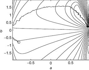
Figure 5.8 Weight convergence trajectory under EDC. Source: Adapted from Ref. [233].