
Information Measures
The concept of information is so rich that there exist various definitions of information measures. Kolmogorov had proposed three methods for defining an information measure: probabilistic method, combinatorial method, and computational method [146]. Accordingly, information measures can be categorized into three categories: probabilistic information (or statistical information), combinatory information, and algorithmic information. This book focuses mainly on statistical information, which was first conceptualized by Shannon [44]. As a branch of mathematical statistics, the establishment of Shannon information theory lays down a mathematical framework for designing optimal communication systems. The core issues in Shannon information theory are how to measure the amount of information and how to describe the information transmission. According to the feature of data transmission in communication, Shannon proposed the use of entropy, which measures the uncertainty contained in a probability distribution, as the definition of information in the data source.
2.1 Entropy
Definition 2.1
Given a discrete random variable ![]() with probability mass function
with probability mass function ![]() ,
, ![]() , Shannon’s (discrete) entropy is defined by [43]
, Shannon’s (discrete) entropy is defined by [43]
![]() (2.1)
(2.1)
where ![]() is Hartley’s amount of information associated with the discrete value
is Hartley’s amount of information associated with the discrete value ![]() with probability
with probability ![]() .1 This information measure was originally devised by Claude Shannon in 1948 to study the amount of information in a transmitted message. Shannon entropy measures the average information (or uncertainty) contained in a probability distribution and can also be used to measure many other concepts, such as diversity, similarity, disorder, and randomness. However, as the discrete entropy depends only on the distribution
.1 This information measure was originally devised by Claude Shannon in 1948 to study the amount of information in a transmitted message. Shannon entropy measures the average information (or uncertainty) contained in a probability distribution and can also be used to measure many other concepts, such as diversity, similarity, disorder, and randomness. However, as the discrete entropy depends only on the distribution ![]() , and takes no account of the values, it is independent of the dynamic range of the random variable. The discrete entropy is unable to differentiate between two random variables that have the same distribution but different dynamic ranges. Actually the discrete random variables with the same entropy may have arbitrarily small or large variance, a typical measure for value dispersion of a random variable.
, and takes no account of the values, it is independent of the dynamic range of the random variable. The discrete entropy is unable to differentiate between two random variables that have the same distribution but different dynamic ranges. Actually the discrete random variables with the same entropy may have arbitrarily small or large variance, a typical measure for value dispersion of a random variable.
Since system parameter identification deals, in general, with continuous random variables, we are more interested in the entropy of a continuous random variable.
Definition 2.2
If ![]() is a continuous random variable with PDF
is a continuous random variable with PDF ![]() ,
, ![]() , Shannon’s differential entropy is defined as
, Shannon’s differential entropy is defined as
![]() (2.2)
(2.2)
The differential entropy is a functional of the PDF ![]() . For this reason, we also denote it by
. For this reason, we also denote it by ![]() . The entropy definition in (2.2) can be extended to multiple random variables. The joint entropy of two continuous random variables
. The entropy definition in (2.2) can be extended to multiple random variables. The joint entropy of two continuous random variables ![]() and
and ![]() is
is
![]() (2.3)
(2.3)
where ![]() denotes the joint PDF of
denotes the joint PDF of ![]() . Furthermore, one can define the conditional entropy of
. Furthermore, one can define the conditional entropy of ![]() given
given ![]() as
as
![]() (2.4)
(2.4)
where ![]() is the conditional PDF of
is the conditional PDF of ![]() given
given ![]() .2
.2
If ![]() and
and ![]() are discrete random variables, the entropy definitions in (2.3) and (2.4) only need to replace the PDFs with the probability mass functions and the integral operation with the summation.
are discrete random variables, the entropy definitions in (2.3) and (2.4) only need to replace the PDFs with the probability mass functions and the integral operation with the summation.
Theorem 2.1
Properties of the differential entropy3 :
1. Differential entropy can be either positive or negative.
2. Differential entropy is not related to the mean value (shift invariant), i.e., ![]() , where
, where ![]() is an arbitrary constant.
is an arbitrary constant.
5. Entropy has the concavity property: ![]() is a concave function of
is a concave function of ![]() , that is,
, that is, ![]() , we have
, we have
![]() (2.5)
(2.5)
6. If random variables ![]() and
and ![]() are mutually independent, then
are mutually independent, then
![]() (2.6)
(2.6)
that is, the entropy of the sum of two independent random variables is no smaller than the entropy of each individual variable.
7. Entropy power inequality (EPI): If ![]() and
and ![]() are mutually independent
are mutually independent ![]() -dimensional random variables, we have
-dimensional random variables, we have
![]() (2.7)
(2.7)
with equality if and only if ![]() and
and ![]() are Gaussian distributed and their covariance matrices are in proportion to each other.
are Gaussian distributed and their covariance matrices are in proportion to each other.
8. Assume ![]() and
and ![]() are two
are two ![]() -dimensional random variables,
-dimensional random variables, ![]() ,
, ![]() denotes a smooth bijective mapping defined over
denotes a smooth bijective mapping defined over ![]() ,
, ![]() is the Jacobi matrix of
is the Jacobi matrix of ![]() , then
, then
![]() (2.8)
(2.8)
where ![]() denotes the determinant.
denotes the determinant.
9. Suppose ![]() is a
is a ![]() -dimensional Gaussian random variable,
-dimensional Gaussian random variable, ![]() , i.e.,
, i.e.,
![]() (2.9)
(2.9)
Then the differential entropy of ![]() is
is
![]() (2.10)
(2.10)
Differential entropy measures the uncertainty and dispersion in a probability distribution. Intuitively, the larger the value of entropy, the more scattered the probability density of a random variable or in other word, the smaller the value of entropy, the more concentrated the probability density. For a one-dimensional random variable, the differential entropy is similar to the variance. For instance, the differential entropy of a one-dimensional Gaussian random variable ![]() is
is ![]() , where
, where ![]() denotes the variance of
denotes the variance of ![]() . It is clear to see that in this case the differential entropy increases monotonically with increasing variance. However, the entropy is in essence quite different from the variance; it is a more comprehensive measure. The variance of some random variable is infinite, while the entropy is still finite. For example, consider the following Cauchy distribution4 :
. It is clear to see that in this case the differential entropy increases monotonically with increasing variance. However, the entropy is in essence quite different from the variance; it is a more comprehensive measure. The variance of some random variable is infinite, while the entropy is still finite. For example, consider the following Cauchy distribution4 :
![]() (2.11)
(2.11)
Its variance is infinite, while the differential entropy is ![]() [147].
[147].
There is an important entropy optimization principle, that is, the maximum entropy (MaxEnt) principle enunciated by Jaynes [148] and Kapur and Kesavan [149]. According to MaxEnt, among all the distributions that satisfy certain constraints, one should choose the distribution that maximizes the entropy, which is considered to be the most objective and most impartial choice. MaxEnt is a powerful and widely accepted principle for statistical inference with incomplete knowledge of the probability distribution.
The maximum entropy distribution under characteristic moment constraints can be obtained by solving the following optimization problem:
 (2.12)
where ![]() is the natural constraint (the normalization constraint) and
is the natural constraint (the normalization constraint) and ![]() (
(![]() ) denote
) denote ![]() (generalized) characteristic moment constraints.
(generalized) characteristic moment constraints.
Theorem 2.2
(Maximum Entropy PDF) Satisfying the constraints in (2.12), the maximum entropy PDF is given by
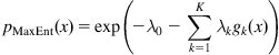 (2.13)
where the coefficients ![]() are the solution of the following equations5:
are the solution of the following equations5:
 (2.14)
In statistical information theory, in addition to Shannon entropy, there are many other definitions of entropy, such as Renyi entropy (named after Alfred Renyi) [152], Havrda–Charvat entropy [153], Varma entropy [154], Arimoto entropy [155], and ![]() -entropy [156]. Among them,
-entropy [156]. Among them, ![]() -entropy is the most generalized definition of entropy.
-entropy is the most generalized definition of entropy. ![]() -entropy of a continuous random variable
-entropy of a continuous random variable ![]() is defined by [156]
is defined by [156]
![]() (2.15)
(2.15)
where either ![]() is a concave function and
is a concave function and ![]() is a monotonously increasing function or
is a monotonously increasing function or ![]() is a convex function and
is a convex function and ![]() is a monotonously decreasing function. When
is a monotonously decreasing function. When ![]() ,
, ![]() -entropy becomes the
-entropy becomes the ![]() -entropy:
-entropy:
![]() (2.16)
(2.16)
where ![]() is a concave function. Similar to Shannon entropy,
is a concave function. Similar to Shannon entropy, ![]() -entropy is also shift-invariant and satisfies (see Appendix C for the proof)
-entropy is also shift-invariant and satisfies (see Appendix C for the proof)
![]() (2.17)
(2.17)
where ![]() and
and ![]() are two mutually independent random variables. Some typical examples of
are two mutually independent random variables. Some typical examples of ![]() -entropy are given in Table 2.1. As one can see, many entropy definitions can be regarded as the special cases of
-entropy are given in Table 2.1. As one can see, many entropy definitions can be regarded as the special cases of ![]() -entropy.
-entropy.

From Table 2.1, Renyi’s entropy of order-![]() is defined as
is defined as
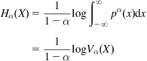 (2.18)
where ![]() ,
, ![]() ,
, ![]() is called the order-
is called the order-![]() information potential (when
information potential (when ![]() , called the quadratic information potential, QIP) [64]. The Renyi entropy is a generalization of Shannon entropy. In the limit
, called the quadratic information potential, QIP) [64]. The Renyi entropy is a generalization of Shannon entropy. In the limit ![]() , it will converge to Shannon entropy, i.e.,
, it will converge to Shannon entropy, i.e., ![]() .
.
The previous entropies are all defined based on the PDFs (for continuous random variable case). Recently, some researchers also propose to define the entropy measure using the distribution or survival functions [157,158]. For example, the cumulative residual entropy (CRE) of a scalar random variable ![]() is defined by [157]
is defined by [157]
![]() (2.19)
(2.19)
where ![]() is the survival function of
is the survival function of ![]() . The CRE is just defined by replacing the PDF with the survival function (of an absolute value transformation of
. The CRE is just defined by replacing the PDF with the survival function (of an absolute value transformation of ![]() ) in the original differential entropy (2.2). Further, the order-
) in the original differential entropy (2.2). Further, the order-![]() (
(![]() ) survival information potential (SIP) is defined as [159]
) survival information potential (SIP) is defined as [159]
![]() (2.20)
(2.20)
This new definition of information potential is valid for both discrete and continuous random variables.
In recent years, the concept of correntropy has also been applied successfully in signal processing and machine learning [137]. The correntropy is not a true entropy measure, but in this book it is still regarded as an information theoretic measure since it is closely related to Renyi’s quadratic entropy (![]() ), that is, the negative logarithm of the sample mean of correntropy (with Gaussian kernel) yields the Parzen estimate of Renyi’s quadratic entropy [64]. Let
), that is, the negative logarithm of the sample mean of correntropy (with Gaussian kernel) yields the Parzen estimate of Renyi’s quadratic entropy [64]. Let ![]() and
and ![]() be two random variables with the same dimensions, the correntropy is defined by
be two random variables with the same dimensions, the correntropy is defined by
![]() (2.21)
(2.21)
where ![]() denotes the expectation operator,
denotes the expectation operator, ![]() is a translation invariant Mercer kernel6, and
is a translation invariant Mercer kernel6, and ![]() denotes the joint distribution function of
denotes the joint distribution function of ![]() . According to Mercer’s theorem, any Mercer kernel
. According to Mercer’s theorem, any Mercer kernel ![]() induces a nonlinear mapping
induces a nonlinear mapping ![]() from the input space (original domain) to a high (possibly infinite) dimensional feature space
from the input space (original domain) to a high (possibly infinite) dimensional feature space ![]() (a vector space in which the input data are embedded), and the inner product of two points
(a vector space in which the input data are embedded), and the inner product of two points ![]() and
and ![]() in
in ![]() can be implicitly computed by using the Mercer kernel (the so-called “kernel trick”) [160–162]. Then the correntropy (2.21) can alternatively be expressed as
can be implicitly computed by using the Mercer kernel (the so-called “kernel trick”) [160–162]. Then the correntropy (2.21) can alternatively be expressed as
![]() (2.22)
(2.22)
where ![]() denotes the inner product in
denotes the inner product in ![]() . From (2.22), one can see that the correntropy is in essence a new measure of the similarity between two random variables, which generalizes the conventional correlation function to feature spaces.
. From (2.22), one can see that the correntropy is in essence a new measure of the similarity between two random variables, which generalizes the conventional correlation function to feature spaces.
2.2 Mutual Information
Definition 2.3
The mutual information between continuous random variables ![]() and
and ![]() is defined as
is defined as
![]() (2.23)
(2.23)
The conditional mutual information between ![]() and
and ![]() , conditioned on random variable
, conditioned on random variable ![]() , is given by
, is given by
![]() (2.24)
(2.24)
For a random vector7![]() (
(![]() ), the mutual information between components is
), the mutual information between components is
![]() (2.25)
(2.25)
Theorem 2.3
Properties of the mutual information:
2. Non-negative, i.e., ![]() , with equality if and only if
, with equality if and only if ![]() and
and ![]() are mutually independent.
are mutually independent.
3. Data processing inequality (DPI): If random variables ![]() ,
, ![]() ,
, ![]() form a Markov chain
form a Markov chain ![]() , then
, then ![]() . Especially, if
. Especially, if ![]() is a function of
is a function of ![]() ,
, ![]() , where
, where ![]() is a measurable mapping from
is a measurable mapping from ![]() to
to ![]() , then
, then ![]() , with equality if
, with equality if ![]() is invertible and
is invertible and ![]() is also a measurable mapping.
is also a measurable mapping.
4. The relationship between mutual information and entropy:
![]() (2.26)
(2.26)
5. Chain rule: Let ![]() be
be ![]() random variables. Then
random variables. Then
![]() (2.27)
(2.27)
6. If ![]() ,
, ![]() ,
, ![]() are
are ![]() ,
, ![]() , and
, and ![]() -dimension Gaussian random variables with, respectively, covariance matrices
-dimension Gaussian random variables with, respectively, covariance matrices ![]() ,
, ![]() , and
, and ![]() , then the mutual information between
, then the mutual information between ![]() and
and ![]() is
is
![]() (2.28)
(2.28)
In particular, if ![]() , we have
, we have
![]() (2.29)
(2.29)
where ![]() denotes the correlation coefficient between
denotes the correlation coefficient between ![]() and
and ![]() .
.
7. Relationship between mutual information and MSE: Assume ![]() and
and ![]() are two Gaussian random variables, satisfying
are two Gaussian random variables, satisfying ![]() , where
, where ![]() ,
, ![]() ,
, ![]() and
and ![]() are mutually independent. Then we have [81]
are mutually independent. Then we have [81]
![]() (2.30)
(2.30)
where ![]() denotes the minimum MSE when estimating
denotes the minimum MSE when estimating ![]() based on
based on ![]() .
.
Mutual information is a measure of the amount of information that one random variable contains about another random variable. The stronger the dependence between two random variables, the greater the mutual information is. If two random variables are mutually independent, the mutual information between them achieves the minimum zero. The mutual information has close relationship with the correlation coefficient. According to (2.29), for two Gaussian random variables, the mutual information is a monotonically increasing function of the correlation coefficient. However, the mutual information and the correlation coefficient are different in nature. The mutual information being zero implies that the random variables are mutually independent, thereby the correlation coefficient is also zero, while the correlation coefficient being zero does not mean the mutual information is zero (i.e., the mutual independence). In fact, the condition of independence is much stronger than mere uncorrelation. Consider the following Pareto distributions [149]:
 (2.31)
where ![]() ,
, ![]() ,
, ![]() . One can calculate
. One can calculate ![]() ,
, ![]() , and
, and ![]() , and hence
, and hence ![]() (
(![]() and
and ![]() are uncorrelated). In this case, however,
are uncorrelated). In this case, however, ![]() , that is,
, that is, ![]() and
and ![]() are not mutually independent (the mutual information not being zero).
are not mutually independent (the mutual information not being zero).
With mutual information, one can define the rate distortion function and the distortion rate function. The rate distortion function ![]() of a random variable
of a random variable ![]() with MSE distortion is defined by
with MSE distortion is defined by
![]() (2.32)
(2.32)
At the same time, the distortion rate function is defined as
![]() (2.33)
(2.33)
Theorem 2.4
If ![]() is a Gaussian random variable,
is a Gaussian random variable, ![]() , then
, then
 (2.34)
2.3 Information Divergence
In statistics and information geometry, an information divergence measures the “distance” of one probability distribution to the other. However, the divergence is a much weaker notion than that of the distance in mathematics, in particular it need not be symmetric and need not satisfy the triangle inequality.
Definition 2.4
Assume that ![]() and
and ![]() are two random variables with PDFs
are two random variables with PDFs ![]() and
and ![]() with common support. The Kullback–Leibler information divergence (KLID) between
with common support. The Kullback–Leibler information divergence (KLID) between ![]() and
and ![]() is defined by
is defined by
![]() (2.35)
(2.35)
In the literature, the KL-divergence is also referred to as the discrimination information, the cross entropy, the relative entropy, or the directed divergence.
Theorem 2.5
Properties of KL-divergence:
1. ![]() , with equality if and only if
, with equality if and only if ![]() .
.
2. Nonsymmetry: In general, we have ![]() .
.
3. ![]() , that is, the mutual information between two random variables is actually the KL-divergence between the joint probability density and the product of the marginal probability densities.
, that is, the mutual information between two random variables is actually the KL-divergence between the joint probability density and the product of the marginal probability densities.
4. Convexity property: ![]() is a convex function of
is a convex function of ![]() , i.e.,
, i.e., ![]() , we have
, we have
![]() (2.36)
(2.36)
where ![]() and
and ![]() .
.
5. Pinsker’s inequality: Pinsker inequality is an inequality that relates KL-divergence and the total variation distance. It states that
![]() (2.37)
(2.37)
6. Invariance under invertible transformation: Given random variables ![]() and
and ![]() , and the invertible transformation
, and the invertible transformation ![]() , the KL-divergence remains unchanged after the transformation, i.e.,
, the KL-divergence remains unchanged after the transformation, i.e., ![]() . In particular, if
. In particular, if ![]() , where
, where ![]() is a constant, then the KL-divergence is shift-invariant:
is a constant, then the KL-divergence is shift-invariant:
![]() (2.38)
(2.38)
7. If ![]() and
and ![]() are two
are two ![]() -dimensional Gaussian random variables,
-dimensional Gaussian random variables, ![]() ,
, ![]() , then
, then
![]() (2.39)
(2.39)
where ![]() denotes the trace operator.
denotes the trace operator.
There are many other definitions of information divergence. Some quadratic divergences are frequently used in machine learning, since they involve only a simple quadratic form of PDFs. Among them, the Euclidean distance (ED) in probability spaces and the Cauchy–Schwarz (CS)-divergence are popular, and are defined respectively as [64]
![]() (2.40)
(2.40)
![]() (2.41)
(2.41)
Clearly, the ED in (2.40) can be expressed in terms of QIP:
![]() (2.42)
(2.42)
where ![]() is named the cross information potential (CIP). Further, the CS-divergence of (2.41) can also be rewritten in terms of Renyi’s quadratic entropy:
is named the cross information potential (CIP). Further, the CS-divergence of (2.41) can also be rewritten in terms of Renyi’s quadratic entropy:
![]() (2.43)
(2.43)
where ![]() is called Renyi’s quadratic cross entropy.
is called Renyi’s quadratic cross entropy.
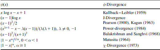
Also, there is a much generalized definition of divergence, i.e., the ![]() -divergence, which is defined as [130]
-divergence, which is defined as [130]
![]() (2.44)
(2.44)
where ![]() is a collection of convex functions,
is a collection of convex functions, ![]() ,
, ![]() ,
, ![]() , and
, and ![]() . When
. When ![]() (or
(or ![]() ), the
), the ![]() -divergence becomes the KL-divergence. It is easy to verify that the
-divergence becomes the KL-divergence. It is easy to verify that the ![]() -divergence satisfies the properties (1), (4), and (6) in Theorem 2.5. Table 2.2 gives some typical examples of
-divergence satisfies the properties (1), (4), and (6) in Theorem 2.5. Table 2.2 gives some typical examples of ![]() -divergence.
-divergence.
2.4 Fisher Information
The most celebrated information measure in statistics is perhaps the one developed by R.A. Fisher (1921) for the purpose of quantifying information in a distribution about the parameter.
Definition 2.5
Given a parameterized PDF ![]() , where
, where ![]() ,
, ![]() is a
is a ![]() -dimensional parameter vector, and assuming
-dimensional parameter vector, and assuming ![]() is continuously differentiable with respect to
is continuously differentiable with respect to ![]() , then the Fisher information matrix (FIM) with respect to
, then the Fisher information matrix (FIM) with respect to ![]() is
is
![]() (2.45)
(2.45)
Clearly, the FIM ![]() , also referred to as the Fisher information, is a
, also referred to as the Fisher information, is a ![]() matrix. If
matrix. If ![]() is a location parameter, i.e.,
is a location parameter, i.e., ![]() , Fisher information will be
, Fisher information will be
![]() (2.46)
(2.46)
The Fisher information of (2.45) can alternatively be written as
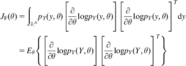 (2.47)
where ![]() stands for the expectation with respect to
stands for the expectation with respect to ![]() . From (2.47), one can see that the Fisher information measures the “average sensitivity” of the logarithm of PDF to the parameter
. From (2.47), one can see that the Fisher information measures the “average sensitivity” of the logarithm of PDF to the parameter ![]() or the “average influence” of the parameter
or the “average influence” of the parameter ![]() on the logarithm of PDF. The Fisher information is also a measure of the minimum error in estimating the parameter of a distribution. This is illustrated in the following theorem.
on the logarithm of PDF. The Fisher information is also a measure of the minimum error in estimating the parameter of a distribution. This is illustrated in the following theorem.
Theorem 2.6
(Cramer–Rao Inequality) Let ![]() be a parameterized PDF, where
be a parameterized PDF, where ![]() ,
, ![]() is a
is a ![]() -dimensional parameter vector, and assume that
-dimensional parameter vector, and assume that ![]() is continuously differentiable with respect to
is continuously differentiable with respect to ![]() . Denote
. Denote ![]() an unbiased estimator of
an unbiased estimator of ![]() based on
based on ![]() , satisfying
, satisfying ![]() , where
, where ![]() denotes the true value of
denotes the true value of ![]() . Then
. Then
![]() (2.48)
(2.48)
where ![]() is the covariance matrix of
is the covariance matrix of ![]() .
.
Cramer–Rao inequality shows that the inverse of the FIM provides a lower bound on the error covariance matrix of the parameter estimator, which plays a significant role in parameter estimation. A proof of the Theorem 2.6 is given in Appendix D.
2.5 Information Rate
The previous information measures, such as entropy, mutual information, and KL-divergence, are all defined for random variables. These definitions can be further extended to various information rates, which are defined for random processes.
Definition 2.6
Let ![]() and
and ![]() be two discrete-time stochastic processes, and denote
be two discrete-time stochastic processes, and denote ![]() ,
, ![]() . The entropy rate of the stochastic process
. The entropy rate of the stochastic process ![]() is defined as
is defined as
![]() (2.49)
(2.49)
The mutual information rate between ![]() and
and ![]() is defined by
is defined by
![]() (2.50)
(2.50)
If ![]() , the KL-divergence rate between
, the KL-divergence rate between ![]() and
and ![]() is
is
![]() (2.51)
(2.51)
If the PDF of the stochastic process ![]() is dependent on and continuously differentiable with respect to the parameter vector
is dependent on and continuously differentiable with respect to the parameter vector ![]() , then the Fisher information rate matrix (FIRM) is
, then the Fisher information rate matrix (FIRM) is
![]() (2.52)
(2.52)
The information rates measure the average amount of information of stochastic processes in unit time. The limitations in Definition 2.6 may not exist, however, if the stochastic processes are stationary, these limitations in general exist. The following theorem gives the information rates for stationary Gaussian processes.
Theorem 2.7
Given two jointly Gaussian stationary processes ![]() and
and ![]() , with power spectral densities
, with power spectral densities ![]() and
and ![]() , and
, and ![]() with spectral density
with spectral density ![]() , the entropy rate of the Gaussian process
, the entropy rate of the Gaussian process ![]() is
is
![]() (2.53)
(2.53)
The mutual information rate between ![]() and
and ![]() is
is
![]() (2.54)
(2.54)
If ![]() , the KL-divergence rate between
, the KL-divergence rate between ![]() and
and ![]() is
is
![]() (2.55)
(2.55)
If the PDF of ![]() is dependent on and continuously differentiable with respect to the parameter vector
is dependent on and continuously differentiable with respect to the parameter vector ![]() , then the FIRM (assuming
, then the FIRM (assuming ![]() ) is [163]
) is [163]
![]() (2.56)
(2.56)
Appendix B  -Stable Distribution
![]() -stable distributions are a class of probability distributions satisfying the generalized central limit theorem, which are extensions of the Gaussian distribution. The Gaussian, inverse Gaussian, and Cauchy distributions are its special cases. Excepting the three kinds of distributions, other
-stable distributions are a class of probability distributions satisfying the generalized central limit theorem, which are extensions of the Gaussian distribution. The Gaussian, inverse Gaussian, and Cauchy distributions are its special cases. Excepting the three kinds of distributions, other ![]() -stable distributions do not have PDF with analytical expression. However, their characteristic functions can be written in the following form:
-stable distributions do not have PDF with analytical expression. However, their characteristic functions can be written in the following form:
 (B.1)
(B.1)
where ![]() is the location parameter,
is the location parameter, ![]() is the dispersion parameter,
is the dispersion parameter, ![]() is the characteristic factor,
is the characteristic factor, ![]() is the skewness factor. The parameter
is the skewness factor. The parameter ![]() determines the trailing of distribution. The smaller the value of
determines the trailing of distribution. The smaller the value of ![]() , the heavier the trail of the distribution is. The distribution is symmetric if
, the heavier the trail of the distribution is. The distribution is symmetric if ![]() , called the symmetric
, called the symmetric ![]() -stable (
-stable (![]() ) distribution. The Gaussian and Cauchy distributions are
) distribution. The Gaussian and Cauchy distributions are ![]() -stable distributions with
-stable distributions with ![]() and
and ![]() , respectively.
, respectively.
When ![]() , the tail attenuation of
, the tail attenuation of ![]() -stable distribution is slower than that of Gaussian distribution, which can be used to describe the outlier data or impulsive noises. In this case the distribution has infinite second-order moment, while the entropy is still finite.
-stable distribution is slower than that of Gaussian distribution, which can be used to describe the outlier data or impulsive noises. In this case the distribution has infinite second-order moment, while the entropy is still finite.
Appendix C Proof of (2.17)
Proof
Assume ![]() is a concave function, and
is a concave function, and ![]() is a monotonically increasing function. Denote
is a monotonically increasing function. Denote ![]() the inverse of function
the inverse of function ![]() , we have
, we have
![]() (C.1)
(C.1)
Since ![]() and
and ![]() are independent, then
are independent, then
![]() (C.2)
(C.2)
According to Jensen’s inequality, we can derive
 (C.3)
(C.3)
As ![]() is monotonically increasing,
is monotonically increasing, ![]() must also be monotonically increasing, thus we have
must also be monotonically increasing, thus we have ![]() . Similarly,
. Similarly, ![]() . Therefore,
. Therefore,
![]() (C.4)
(C.4)
For the case in which ![]() is a convex function and
is a convex function and ![]() is monotonically decreasing, the proof is similar (omitted).
is monotonically decreasing, the proof is similar (omitted).
Appendix D Proof of Cramer–Rao Inequality
Proof
First, one can derive the following two equalities:
 (D.1)
(D.1)
 (D.2)
(D.2)
where ![]() is a
is a ![]() identity matrix. Denote
identity matrix. Denote ![]() and
and ![]() .
.
Then
 (D.3)
(D.3)
So we obtain
![]() (D.4)
(D.4)
According to the matrix theory, if the symmetric matrix ![]() is positive-definite, then
is positive-definite, then ![]() . It follows that
. It follows that
![]() (D.5)
(D.5)
i.e., ![]() .
.
1In this book, “log” always denotes the natural logarithm. The entropy will then be measured in nats.
2Strictly speaking, we should use some subscripts to distinguish the PDFs ![]() ,
, ![]() , and
, and ![]() . For example, we can write them as
. For example, we can write them as ![]() ,
, ![]() ,
, ![]() . In this book, for simplicity we often omit these subscripts if no confusion arises.
. In this book, for simplicity we often omit these subscripts if no confusion arises.
3The detailed proofs of these properties can be found in related information theory textbooks, such as “Elements of Information Theory” written by Cover and Thomas [43].
4Cauchy distribution is a non-Gaussian ![]() -stable distribution (see Appendix B).
-stable distribution (see Appendix B).
5On how to solve these equations, interested readers are referred to [150,151].
6Let ![]() be a measurable space and assume a real-valued function
be a measurable space and assume a real-valued function ![]() is defined on
is defined on ![]() , i.e.,
, i.e., ![]() . Then function
. Then function ![]() is called a Mercer kernel if and only if it is a continuous, symmetric, and positive-definite function. Here,
is called a Mercer kernel if and only if it is a continuous, symmetric, and positive-definite function. Here, ![]() is said to be positive-definite if and only if
is said to be positive-definite if and only if
![]()
where ![]() denotes any finite signed Borel measure,
denotes any finite signed Borel measure, ![]() . If the equality holds only for zero measure, then
. If the equality holds only for zero measure, then ![]() is said to be strictly positive-definite (SPD).
is said to be strictly positive-definite (SPD).
7Unless mentioned otherwise, in this book a vector refers to a column vector.