
System Identification Under Minimum Error Entropy Criteria
In previous chapter, we give an overview of information theoretic parameter estimation. These estimation methods are, however, devoted to cases where a large amount of statistical information on the unknown parameter is assumed to be available. For example, the minimum divergence estimation needs to know the likelihood function of the parameter. Also, in Bayes estimation with minimum error entropy (MEE) criterion, the joint distribution of unknown parameter and observation is assumed to be known. In this and later chapters, we will further investigate information theoretic system identification. Our focus is mainly on system parameter estimation (identification) where no statistical information on parameters exists (i.e., only data samples are available). To develop the identification algorithms under information theoretic criteria, one should evaluate the related information measures. This requires the knowledge of the data distributions, which are, in general, unknown to us. To address this issue, we can use the estimated (empirical) information measures as the identification criteria.
4.1 Brief Sketch of System Parameter Identification
System identification involves fitting the experimental input–output data (training data) into empirical model. In general, system identification includes the following key steps:
• Experiment design: To obtain good experimental data. Usually, the input signals should be designed such that it provides enough process excitation.
• Selection of model structure: To choose a suitable model structure based on the training data or prior knowledge.
• Selection of the criterion: To choose a suitable criterion (cost) function that reflects how well the model fits the experimental data.
• Parameter identification: To obtain the model parameters1 by optimizing (minimizing or maximizing) the above criterion function.
• Model validation: To test the model so as to reveal any inadequacies.
In this book, we focus mainly on the parameter identification part. Figure 4.1 shows a general scheme of discrete-time system identification, where ![]() and
and ![]() denote the system input and output (clean output) at time
denote the system input and output (clean output) at time ![]() ,
, ![]() is an additive noise that accounts for the system uncertainty or measurement error, and
is an additive noise that accounts for the system uncertainty or measurement error, and ![]() is the measured output. Further,
is the measured output. Further, ![]() is the model output and
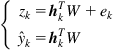
is the model output and ![]() denotes the identification error, which is defined as the difference between the measured output and the model output, i.e.,
denotes the identification error, which is defined as the difference between the measured output and the model output, i.e., ![]() . The goal of parameter identification is then to search the model parameter vector (or weight vector) so as to minimize (or maximize) a certain criterion function (usually the model structure is predefined).
. The goal of parameter identification is then to search the model parameter vector (or weight vector) so as to minimize (or maximize) a certain criterion function (usually the model structure is predefined).

The implementation of system parameter identification involves model structure, criterion function, and parameter search (identification) algorithm. In the following, we will briefly discuss these three aspects.
4.1.1 Model Structure
Generally speaking, the model structure is a parameterized mapping from inputs2 to outputs. There are various mathematical descriptions of system model (linear or nonlinear, static or dynamic, deterministic or stochastic, etc.). Many of them can be expressed as the following linear-in-parameter model:
 (4.1)
(4.1)
where ![]() denotes the regression input vector and
denotes the regression input vector and ![]() denotes the weight vector (i.e., parameter vector). The simplest linear-in-parameter model is the adaptive linear neuron (ADALINE). Let the input be an
denotes the weight vector (i.e., parameter vector). The simplest linear-in-parameter model is the adaptive linear neuron (ADALINE). Let the input be an ![]() -dimensional vector
-dimensional vector ![]() . The output of ADALINE model will be
. The output of ADALINE model will be
![]() (4.2)
(4.2)
where ![]() is a bias (some constant). In this case, we have
is a bias (some constant). In this case, we have
 (4.3)
(4.3)
If the bias ![]() is zero, and the input vector is
is zero, and the input vector is ![]() , which is formed by feeding the input signal to a tapped delay line, then the ADALINE becomes a finite impulse response (FIR) filter.
, which is formed by feeding the input signal to a tapped delay line, then the ADALINE becomes a finite impulse response (FIR) filter.
The ARX (autoregressive with external input) dynamic model is another important linear-in-parameter model:
![]() (4.4)
(4.4)
One can write Eq. (4.4) as ![]() if let
if let
 (4.5)
(4.5)
The linear-in-parameter model also includes many nonlinear models as special cases. For example, the ![]() -order polynomial model can be expressed as
-order polynomial model can be expressed as
![]() (4.6)
(4.6)
where
 (4.7)
(4.7)
Other examples include: the discrete-time Volterra series with finite memory and order, Hammerstein model, radial basis function (RBF) neural networks with fixed centers, and so on.
In most cases, the system model is a nonlinear-in-parameter model, whose output is not linearly related to the parameters. A typical example of nonlinear-in-parameter model is the multilayer perceptron (MLP) [53]. The MLP, with one hidden layer, can be generally expressed as follows:
![]() (4.8)
(4.8)
where ![]() is the
is the ![]() input vector,
input vector, ![]() is the
is the ![]() weight matrix connecting the input layer with the hidden layer,
weight matrix connecting the input layer with the hidden layer, ![]() is the activation function (usually a sigmoid function),
is the activation function (usually a sigmoid function), ![]() is the
is the ![]() bias vector for the hidden neurons,
bias vector for the hidden neurons, ![]() is the
is the ![]() weight vector connecting the hidden layer to the output neuron, and
weight vector connecting the hidden layer to the output neuron, and ![]() is the bias for the output neuron.
is the bias for the output neuron.
The model can also be created in kernel space. In kernel machine learning (e.g. support vector machine, SVM), one often uses a reproducing kernel Hilbert space (RKHS) ![]() associated with a Mercer kernel
associated with a Mercer kernel ![]() as the hypothesis space [161, 162]. According to Moore-Aronszajn theorem [174, 175], every Mercer kernel
as the hypothesis space [161, 162]. According to Moore-Aronszajn theorem [174, 175], every Mercer kernel ![]() induces a unique function space
induces a unique function space ![]() , namely the RKHS, whose reproducing kernel is
, namely the RKHS, whose reproducing kernel is ![]() , satisfying: 1)
, satisfying: 1) ![]() , the function
, the function ![]() , and 2)
, and 2) ![]() , and for every
, and for every ![]() ,
, ![]() , where
, where ![]() denotes the inner product in
denotes the inner product in ![]() . If Mercer kernel
. If Mercer kernel ![]() is strictly positive-definite, the induced RKHS
is strictly positive-definite, the induced RKHS ![]() will be universal (dense in the space of continuous functions over
will be universal (dense in the space of continuous functions over ![]() ). Assuming the input signal
). Assuming the input signal ![]() , the model in RKHS
, the model in RKHS ![]() can be expressed as
can be expressed as
![]() (4.9)
(4.9)
where ![]() is the unknown input–output mapping that needs to be estimated. This model is a nonparametric function over input space
is the unknown input–output mapping that needs to be estimated. This model is a nonparametric function over input space ![]() . However, one can regard it as a “parameterized” model, where the parameter space is the RKHS
. However, one can regard it as a “parameterized” model, where the parameter space is the RKHS ![]() .
.
The model (4.9) can alternatively be expressed in a feature space (a vector space in which the training data are embedded). According to Mercer’s theorem, any Mercer kernel ![]() induces a mapping
induces a mapping ![]() from the input space
from the input space ![]() to a feature space
to a feature space ![]() .3 In the feature space, the inner products can be calculated using the kernel evaluation:
.3 In the feature space, the inner products can be calculated using the kernel evaluation:
![]() (4.10)
(4.10)
The feature space ![]() is isometric-isomorphic to the RKHS
is isometric-isomorphic to the RKHS ![]() . This can be easily understood by identifying
. This can be easily understood by identifying ![]() and
and ![]() , where
, where ![]() denotes a vector in feature space
denotes a vector in feature space ![]() , satisfying
, satisfying ![]() ,
, ![]() . Therefore, in feature space the model (4.9) becomes
. Therefore, in feature space the model (4.9) becomes
![]() (4.11)
(4.11)
This is a linear model in feature space, with ![]() as the input, and
as the input, and ![]() as the weight vector. It is worth noting that the model (4.11) is actually a nonlinear model in input space, since the mapping
as the weight vector. It is worth noting that the model (4.11) is actually a nonlinear model in input space, since the mapping ![]() is in general a nonlinear mapping. The key principle behind kernel method is that, as long as a linear model (or algorithm) in high-dimensional feature space can be formulated in terms of inner products, a nonlinear model (or algorithm) can be obtained by simply replacing the inner product with a Mercer kernel. The model (4.11) can also be regarded as a “parameterized” model in feature space, where the parameter is the weight vector
is in general a nonlinear mapping. The key principle behind kernel method is that, as long as a linear model (or algorithm) in high-dimensional feature space can be formulated in terms of inner products, a nonlinear model (or algorithm) can be obtained by simply replacing the inner product with a Mercer kernel. The model (4.11) can also be regarded as a “parameterized” model in feature space, where the parameter is the weight vector ![]() .
.
4.1.2 Criterion Function
The criterion (risk or cost) function in system identification reflects how well the model fits the experimental data. In most cases, the criterion is a functional of the identification error ![]() , with the form
, with the form
![]() (4.12)
(4.12)
where ![]() is a loss function, which usually satisfies
is a loss function, which usually satisfies
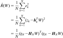
Typical examples of criterion (4.12) include the mean square error (MSE), mean absolute deviation (MAD), mean ![]() -power error (MPE), and so on. In practice, the error distribution is in general unknown, and hence, we have to estimate the expectation value in Eq. (4.12) using sample data. The estimated criterion function is called the empirical criterion function (empirical risk). Given a loss function
-power error (MPE), and so on. In practice, the error distribution is in general unknown, and hence, we have to estimate the expectation value in Eq. (4.12) using sample data. The estimated criterion function is called the empirical criterion function (empirical risk). Given a loss function ![]() , the empirical criterion function
, the empirical criterion function ![]() can be computed as follows:
can be computed as follows:
Note that for MSE criterion (![]() ), the average criterion function is the well-known least-squares criterion function (sum of the squared errors).
), the average criterion function is the well-known least-squares criterion function (sum of the squared errors).
Besides the criterion functions of form (4.12), there are many other criterion functions for system identification. In this chapter, we will discuss system identification under MEE criterion.
4.1.3 Identification Algorithm
Given a parameterized model, the identification error ![]() can be expressed as a function of the parameters. For example, for the linear-in-parameter model (4.1), we have
can be expressed as a function of the parameters. For example, for the linear-in-parameter model (4.1), we have
![]() (4.13)
(4.13)
which is a linear function of ![]() (assuming
(assuming ![]() and
and ![]() are known). Similarly, the criterion function
are known). Similarly, the criterion function ![]() (or the empirical criterion function
(or the empirical criterion function ![]() ) can also be expressed as a function of the parameters, denoted by
) can also be expressed as a function of the parameters, denoted by ![]() (or
(or ![]() ). Therefore, the identification criterion represents a hyper-surface in the parameter space, which is called the performance surface.
). Therefore, the identification criterion represents a hyper-surface in the parameter space, which is called the performance surface.
The parameter ![]() can be identified through searching the optima (minima or maxima) of the performance surface. There are two major ways to do this. One is the batch mode and the other is the online (sequential) mode.
can be identified through searching the optima (minima or maxima) of the performance surface. There are two major ways to do this. One is the batch mode and the other is the online (sequential) mode.
4.1.3.1 Batch Identification
In batch mode, the identification of parameters is done only after collecting a number of samples or even possibly the whole training data. When these data are available, one can calculate the empirical criterion function ![]() based on the model structure. And then, the parameter
based on the model structure. And then, the parameter ![]() can be estimated by solving the following optimization problem:
can be estimated by solving the following optimization problem:
![]() (4.14)
(4.14)
where ![]() denotes the set of all possible values of
denotes the set of all possible values of ![]() . Sometimes, one can achieve an analytical solution by setting the gradient4 of
. Sometimes, one can achieve an analytical solution by setting the gradient4 of ![]() to zero, i.e.,
to zero, i.e.,
![]() (4.15)
(4.15)
For example, with the linear-in-parameter model (4.1) and under the least-squares criterion (empirical MSE criterion), we have
 (4.16)
where ![]() and
and ![]() . And hence,
. And hence,
 (4.17)
If ![]() is a nonsingular matrix, we have
is a nonsingular matrix, we have
![]() (4.18)
(4.18)
In many situations, however, there is no analytical solution for ![]() , and we have to rely on nonlinear optimization techniques, such as gradient descent methods, simulated annealing methods, and genetic algorithms (GAs).
, and we have to rely on nonlinear optimization techniques, such as gradient descent methods, simulated annealing methods, and genetic algorithms (GAs).
The batch mode approach has some shortcomings: (i) it is not suitable for online applications, since the identification is performed only after a number of data are available and (ii) the memory and computational requirements will increase dramatically with the increasing amount of data.
4.1.3.2 Online Identification
The online mode identification is also referred to as the sequential or incremental identification, or adaptive filtering. Compared with the batch mode identification, the sequential identification has some desirable features: (i) the training data (examples or observations) are sequentially (one by one) presented to the identification procedure; (ii) at any time, only few (usually one) training data are used; (iii) a training observation can be discarded as long as the identification procedure for that particular observation is completed; and (iv) it is not necessary to know how many total training observations will be presented. In this book, our focus is primarily on the sequential identification.
The sequential identification is usually performed by means of iterative schemes of the type
![]() (4.19)
(4.19)
where ![]() denotes the estimated parameter at
denotes the estimated parameter at ![]() instant (iteration) and
instant (iteration) and ![]() denotes the adjustment (correction) term. In the following, we present several simple online identification (adaptive filtering) algorithms.
denotes the adjustment (correction) term. In the following, we present several simple online identification (adaptive filtering) algorithms.
4.1.3.3 Recursive Least Squares Algorithm
Given a linear-in-parameter model, the Recursive Least Squares (RLS) algorithm recursively finds the least-squares solution of Eq. (4.18). With a sequence of observations ![]() up to and including time
up to and including time ![]() , the least-squares solution is
, the least-squares solution is
![]() (4.20)
(4.20)
When a new observation ![]() becomes available, the parameter estimate
becomes available, the parameter estimate ![]() is
is
![]() (4.21)
(4.21)
One can derive the following relation between ![]() and
and ![]() :
:
![]() (4.22)
(4.22)
where ![]() is the prediction error,
is the prediction error,
![]() (4.23)
(4.23)
and ![]() is the gain vector, computed as
is the gain vector, computed as
![]() (4.24)
(4.24)
where the matrix ![]() can be calculated recursively as follows:
can be calculated recursively as follows:
![]() (4.25)
(4.25)
Equations (4.22)–(4.25) constitute the RLS algorithm.
Compared to most of its competitors, the RLS exhibits very fast convergence. However, this benefit is achieved at the cost of high computational complexity. If the dimension of ![]() is
is ![]() , then the time and memory complexities of RLS are both
, then the time and memory complexities of RLS are both ![]() .
.
4.1.3.4 Least Mean Square Algorithm
The Least Mean Square (LMS) algorithm is much simpler than RLS, which is a stochastic gradient descent algorithm under the instantaneous MSE cost ![]() . The weight update equation for LMS can be simply derived as follows:
. The weight update equation for LMS can be simply derived as follows:
 (4.26)
where ![]() is the step-size (adaptation gain, learning rate, etc.),5 and the term
is the step-size (adaptation gain, learning rate, etc.),5 and the term ![]() is the instantaneous gradient of the model output with respect to the weight vector, whose form depends on the model structure. For a FIR filter (or ADALINE), the instantaneous gradient will simply be the input vector
is the instantaneous gradient of the model output with respect to the weight vector, whose form depends on the model structure. For a FIR filter (or ADALINE), the instantaneous gradient will simply be the input vector ![]() . In this case, the LMS algorithm becomes6
. In this case, the LMS algorithm becomes6
![]() (4.27)
(4.27)
The computational complexity of the LMS (4.27) is just ![]() , where
, where ![]() is the input dimension.
is the input dimension.
If the model is an MLP network, the term ![]() can be computed by back propagation (BP), which is a common method of training artificial neural networks so as to minimize the objective function [53].
can be computed by back propagation (BP), which is a common method of training artificial neural networks so as to minimize the objective function [53].
There are many other stochastic gradient descent algorithms that are similar to the LMS. Typical examples include the least absolute deviation (LAD) algorithm [31] and the least mean fourth (LMF) algorithm [26]. The LMS, LAD, and LMF algorithms are all special cases of the least mean ![]() -power (LMP) algorithm [30]. The LMP algorithm aims to minimize the
-power (LMP) algorithm [30]. The LMP algorithm aims to minimize the ![]() -power of the error, which can be derived as
-power of the error, which can be derived as
 (4.28)
For the cases ![]() , the above algorithm corresponds to the LAD, LMS, and LMF algorithms, respectively.
, the above algorithm corresponds to the LAD, LMS, and LMF algorithms, respectively.
4.1.3.5 Kernel Adaptive Filtering Algorithms
The kernel adaptive filtering (KAF) algorithms are a family of nonlinear adaptive filtering algorithms developed in kernel (or feature) space [12], by using the linear structure and inner product of this space to implement the well-established linear adaptive filtering algorithms (e.g., LMS, RLS, etc.) and to obtain nonlinear filters in the original input space. They have several desirable features: (i) if choosing a universal kernel (e.g., Gaussian kernel), they are universal approximators; (ii) under MSE criterion, the performance surface is quadratic in feature space so gradient descent learning does not suffer from local minima; and (iii) if pruning the redundant features, they have moderate complexity in terms of computation and memory. Typical KAF algorithms include the kernel recursive least squares (KRLS) [176], kernel least mean square (KLMS) [177], kernel affine projection algorithms (KAPA) [178], and so on. When the kernel is radial (such as the Gaussian kernel), they naturally build a growing RBF network, where the weights are directly related to the errors at each sample. In the following, we only discuss the KLMS algorithm. Interesting readers can refer to Ref. [12] for further information about KAF algorithms.
Let ![]() be an
be an ![]() -dimensional input vector. We can transform
-dimensional input vector. We can transform ![]() into a high-dimensional feature space
into a high-dimensional feature space ![]() (induced by kernel
(induced by kernel ![]() ) through a nonlinear mapping
) through a nonlinear mapping ![]() , i.e.,
, i.e., ![]() . Suppose the model in feature space is given by Eq. (4.11). Then using the LMS algorithm on the transformed observation sequence
. Suppose the model in feature space is given by Eq. (4.11). Then using the LMS algorithm on the transformed observation sequence ![]() yields [177]
yields [177]
 (4.29)
where ![]() denotes the estimated weight vector (at iteration
denotes the estimated weight vector (at iteration ![]() ) in feature space. The KLMS (4.29) is very similar to the LMS algorithm, except for the dimensionality (or richness) of the projection space. The learned mapping (model) at iteration
) in feature space. The KLMS (4.29) is very similar to the LMS algorithm, except for the dimensionality (or richness) of the projection space. The learned mapping (model) at iteration ![]() is the composition of
is the composition of ![]() and
and ![]() , i.e.,
, i.e., ![]() . If identifying
. If identifying ![]() , we obtain the sequential learning rule in the original input space:
, we obtain the sequential learning rule in the original input space:
 (4.30)
At iteration ![]() , given an input
, given an input ![]() , the output of the filter is
, the output of the filter is
![]() (4.31)
(4.31)
From Eq. (4.31) we see that, if choosing a radial kernel, the KLMS produces a growing RBF network by allocating a new kernel unit for every new example with input ![]() as the center and
as the center and ![]() as the coefficient. The algorithm of KLMS is summarized in Table 4.1, and the corresponding network topology is illustrated in Figure 4.2.
as the coefficient. The algorithm of KLMS is summarized in Table 4.1, and the corresponding network topology is illustrated in Figure 4.2.


Selecting a proper Mercer kernel is crucial for all kernel methods. In KLMS, the kernel is usually chosen to be a normalized Gaussian kernel:
![]() (4.32)
(4.32)
where ![]() is the kernel size (kernel width) and
is the kernel size (kernel width) and ![]() is called the kernel parameter. The kernel size in Gaussian kernel is an important parameter that controls the degree of smoothing and consequently has significant influence on the learning performance. Usually, the kernel size can be set manually or estimated in advance by Silverman’s rule [97]. The role of the step-size in KLMS remains in principle the same as the step-size in traditional LMS algorithm. Specifically, it controls the compromise between convergence speed and misadjustment. It has also been shown in Ref. [177] that the step-size in KLMS plays a similar role as the regularization parameter.
is called the kernel parameter. The kernel size in Gaussian kernel is an important parameter that controls the degree of smoothing and consequently has significant influence on the learning performance. Usually, the kernel size can be set manually or estimated in advance by Silverman’s rule [97]. The role of the step-size in KLMS remains in principle the same as the step-size in traditional LMS algorithm. Specifically, it controls the compromise between convergence speed and misadjustment. It has also been shown in Ref. [177] that the step-size in KLMS plays a similar role as the regularization parameter.
The main bottleneck of KLMS (as well as other KAF algorithms) is the linear growing network with each new sample, which poses both computational and memory issues especially for continuous adaptation scenarios. In order to curb the network growth and to obtain a compact representation, a variety of sparsification techniques can be applied, where only the important input data are accepted as the centers. Typical sparsification criteria include the novelty criterion [179], approximate linear dependency (ALD) criterion [176], coherence criterion [180], surprise criterion [181], and so on. The idea of quantization can also be used to yield a compact network with desirable accuracy [182].
4.2 MEE Identification Criterion
Most of the existing approaches to parameter identification utilized the MSE (or equivalently, Gaussian likelihood) as the identification criterion function. The MSE is mathematically tractable and under Gaussian assumption is an optimal criterion for linear system. However, it is well known that MSE may be a poor descriptor of optimality for nonlinear and non-Gaussian (e.g., multimodal, heavy-tail, or finite range distributions) situations, since it constrains only the second-order statistics. To address this issue, one can select some criterion beyond second-order statistics that does not suffer from the limitation of Gaussian assumption and can improve performance in many realistic scenarios. Information theoretic quantities (entropy, divergence, mutual information, etc.) as identification criteria attract ever-increasing attention to this end, since they can capture higher order statistics and information content of signals rather than simply their energy [64]. In the following, we discuss the MEE criterion for system identification.
Under MEE criterion, the parameter vector (weight vector) ![]() can be identified by solving the following optimization problem:
can be identified by solving the following optimization problem:
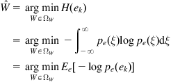 (4.33)
where ![]() denotes the probability density function (PDF) of error
denotes the probability density function (PDF) of error ![]() . If using the order-
. If using the order-![]() Renyi entropy (
Renyi entropy (![]() ,
, ![]() ) of the error as the criterion function, the estimated parameter will be
) of the error as the criterion function, the estimated parameter will be
 (4.34)
where ![]() follows from the monotonicity of logarithm function,
follows from the monotonicity of logarithm function, ![]() is the order-
is the order-![]() information potential (IP) of the error
information potential (IP) of the error ![]() . If
. If ![]() , minimizing the order-
, minimizing the order-![]() Renyi entropy is equivalent to minimizing the order-
Renyi entropy is equivalent to minimizing the order-![]() IP; while if
IP; while if ![]() , minimizing the order-
, minimizing the order-![]() Renyi entropy is equivalent to maximizing the order-
Renyi entropy is equivalent to maximizing the order-![]() IP. In practical application, we often use the order-
IP. In practical application, we often use the order-![]() IP instead of the order-
IP instead of the order-![]() Renyi entropy as the criterion function for identification.
Renyi entropy as the criterion function for identification.
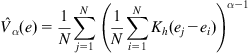
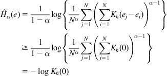
Further, if using the ![]() -entropy of the error as the criterion function, we have
-entropy of the error as the criterion function, we have
 (4.35)
where ![]() . Note that the
. Note that the ![]() -entropy criterion includes the Shannon entropy (
-entropy criterion includes the Shannon entropy (![]() ) and order-
) and order-![]() information potential (
information potential (![]() ) as special cases.
) as special cases.
The error entropy is a functional of error distribution. In practice, the error distribution is usually unknown to us, and so is the error entropy. And hence, we have to estimate the error entropy from error samples, and use the estimated error entropy (called the empirical error entropy) as a criterion to identify the system parameter. In the following, we present several common approaches to estimating the entropy from sample data.
4.2.1 Common Approaches to Entropy Estimation
A straight way to estimate the entropy is to estimate the underlying distribution based on available samples, and plug the estimated distributions into the entropy expression to obtain the entropy estimate (the so-called “plug-in approach”) [183]. Several plug-in estimates of the Shannon entropy (extension to other entropy definitions is straightforward) are presented as follows.
4.2.1.1 Integral Estimate
Denote ![]() the estimated PDF based on sample
the estimated PDF based on sample ![]() . Then the integral estimate of entropy is of the form
. Then the integral estimate of entropy is of the form
![]() (4.36)
(4.36)
where ![]() is a set typically used to exclude the small or tail values of
is a set typically used to exclude the small or tail values of ![]() . The evaluation of Eq. (4.36) requires numerical integration and is not an easy task in general.
. The evaluation of Eq. (4.36) requires numerical integration and is not an easy task in general.
4.2.1.2 Resubstitution Estimate
The resubstitution estimate substitutes the estimated PDF into the sample mean approximation of the entropy measure (approximating the expectation value by its sample mean), which is of the form
![]() (4.37)
(4.37)
This estimation method is considerably simpler than the integral estimate, since it involves no numerical integration.
4.2.1.3 Splitting Data Estimate
Here, we decompose the sample ![]() into two sub samples:
into two sub samples: ![]() ,
, ![]() ,
, ![]() . Based on subsample
. Based on subsample ![]() , we obtain a density estimate
, we obtain a density estimate ![]() , and then, using this density estimate and the second subsample
, and then, using this density estimate and the second subsample ![]() , we estimate the entropy by
, we estimate the entropy by
![]() (4.38)
(4.38)
where ![]() is the indicator function and the set
is the indicator function and the set ![]() (
(![]() ). The splitting data estimate is different from the resubstitution estimate in that it uses different samples to estimate the density and to calculate the sample mean.
). The splitting data estimate is different from the resubstitution estimate in that it uses different samples to estimate the density and to calculate the sample mean.
4.2.1.4 Cross-validation Estimate
If ![]() denotes a density estimate based on sample
denotes a density estimate based on sample ![]() (i.e., leaving
(i.e., leaving ![]() out), then the cross-validation estimate of entropy is
out), then the cross-validation estimate of entropy is
![]() (4.39)
(4.39)
A key step in plug-in estimation is to estimate the PDF from sample data. In the literature, there are mainly two approaches for estimating the PDF of a random variable based on its sample data: parametric and nonparametric. Accordingly, there are also parametric and nonparametric entropy estimations. The parametric density estimation assumes a parametric model of the density and estimates the involved parameters using classical estimation methods like the maximum likelihood (ML) estimation. This approach needs to select a suitable parametric model of the density, which depends upon some prior knowledge. The nonparametric density estimation, however, does not need to select a parametric model, and can estimate the PDF of any distribution.
The histogram density estimation (HDE) and kernel density estimation (KDE) are two popular nonparametric density estimation methods. Here we only discuss the KDE method (also referred to as Parzen window method), which has been widely used in nonparametric regression and pattern recognition. Given a set of independent and identically distributed (i.i.d.) samples7 ![]() drawn from
drawn from ![]() , the KDE for
, the KDE for ![]() is given by [97]
is given by [97]
![]() (4.40)
(4.40)
where ![]() denotes a kernel function8 with width
denotes a kernel function8 with width ![]() , satisfying the following conditions:
, satisfying the following conditions:
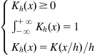 (4.41)
where ![]() is the kernel function with width 1. To make the estimated PDF smooth, the kernel function is usually selected to be a continuous and differentiable (and preferably symmetric and unimodal) function. The most widely used kernel function in KDE is the Gaussian function:
is the kernel function with width 1. To make the estimated PDF smooth, the kernel function is usually selected to be a continuous and differentiable (and preferably symmetric and unimodal) function. The most widely used kernel function in KDE is the Gaussian function:
![]() (4.42)
(4.42)
The kernel width of the Gaussian kernel can be optimized by the ML principle, or selected according to rules-of-thumb, such as Silverman’s rule [97].
With a fixed kernel width ![]() , we have
, we have
![]() (4.43)
(4.43)
where ![]() denotes the convolution operator. Using a suitable annealing rate for the kernel width, the KDE can be asymptotically unbiased and consistent. Specifically, if
denotes the convolution operator. Using a suitable annealing rate for the kernel width, the KDE can be asymptotically unbiased and consistent. Specifically, if ![]() and
and ![]() , then
, then ![]() in probability [98].
in probability [98].
In addition to the plug-in methods described previously, there are many other methods for entropy estimation, such as the sample-spacing method and the nearest neighbor method. In the following, we derive the sample-spacing estimate. First, let us express the Shannon entropy as [184]
![]() (4.44)
(4.44)
where ![]() . Using the slope of the curve
. Using the slope of the curve ![]() to approximate the derivative, we have
to approximate the derivative, we have
![]() (4.45)
(4.45)
where ![]() is the order statistics of the sample
is the order statistics of the sample ![]() , and
, and ![]() is the
is the ![]() -order sample spacing (
-order sample spacing (![]() ). Hence, the sample-spacing estimate of the entropy is
). Hence, the sample-spacing estimate of the entropy is
![]() (4.46)
(4.46)
If adding a correction term to compensate the asymptotic bias, we get
![]() (4.47)
(4.47)
where ![]() is the Digamma function (
is the Digamma function (![]() is the Gamma function).
is the Gamma function).
4.2.2 Empirical Error Entropies Based on KDE
To calculate the empirical error entropy, we usually adopt the resubstitution estimation method with error PDF estimated by KDE. This approach has some attractive features: (i) it is a nonparametric method, and hence requires no prior knowledge on the error distribution; (ii) it is computationally simple, since no numerical integration is needed; and (iii) if choosing a smooth and differentiable kernel function, the empirical error entropy (as a function of the error sample) is also smooth and differentiable (this is very important for the calculation of the gradient).
Suppose now a set of error samples ![]() are available. By KDE, the error density can be estimated as
are available. By KDE, the error density can be estimated as
![]() (4.48)
(4.48)
Then by resubstitution estimation method, we obtain the following empirical error entropies:
 (4.49)
2. Empirical order-![]() Renyi entropy
Renyi entropy
 (4.50)
where ![]() is the empirical order-
is the empirical order-![]() IP, i.e.,
IP, i.e.,
 (4.51)
 (4.52)
It is worth noting that for quadratic information potential (QIP) (![]() ), if choosing Gaussian kernel function, the resubstitution estimate will be identical to the integral estimate but with kernel width
), if choosing Gaussian kernel function, the resubstitution estimate will be identical to the integral estimate but with kernel width ![]() instead of
instead of ![]() . Specifically, if
. Specifically, if ![]() is given by Eq. (4.42), we can derive
is given by Eq. (4.42), we can derive
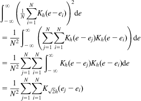 (4.53)
This result comes from the fact that the integral of the product of two Gaussian functions can be exactly evaluated as the value of the Gaussian function computed at the difference of the arguments and whose variance is the sum of the variances of the two original Gaussian functions. From Eq. (4.53), we also see that the QIP can be simply calculated by the double summation over error samples. Due to this fact, when using order-![]() IP, we usually set
IP, we usually set ![]() .
.
In the following, we present some important properties of the empirical error entropy, and our focus is mainly on the order-![]() Renyi entropy (or order-
Renyi entropy (or order-![]() IP) [64,67].
IP) [64,67].
Property 1:
![]() .
.
Proof:
Let ![]() , where
, where ![]() is an arbitrary constant,
is an arbitrary constant, ![]() , then we have
, then we have
 (4.54)
Property 2:
![]() , where
, where  is the empirical Shannon entropy.

Property 3:
Let’s denote ![]() (
(![]() is the kernel width). Then
is the kernel width). Then ![]() ,
, ![]() , we have
, we have ![]() .
.

where (a) is because that ![]() , the kernel function
, the kernel function ![]() satisfies
satisfies ![]() .
.
Property 4:
![]() , where
, where ![]() is a random variable with PDF
is a random variable with PDF ![]() (
(![]() denotes the convolution operator).
denotes the convolution operator).
Proof:
According to the theory of KDE [97,98], we have
![]() (4.57)
(4.57)
Hence, ![]() . Since the PDF of the sum of two independent random variables is equal to the convolution of their individual PDFs,
. Since the PDF of the sum of two independent random variables is equal to the convolution of their individual PDFs, ![]() can be considered as the sum of the error
can be considered as the sum of the error ![]() and another random variable that is independent of the error and has PDF
and another random variable that is independent of the error and has PDF ![]() . And since the entropy of the sum of two independent random variables is no less than the entropy of each individual variable, we have
. And since the entropy of the sum of two independent random variables is no less than the entropy of each individual variable, we have ![]() .
.
Property 5:
If ![]() , then
, then ![]() , with equality if
, with equality if ![]() .
.
Proof:
Consider the case where ![]() (
(![]() is similar), we have
is similar), we have
 (4.58)
If ![]() ,
, ![]() , i.e.,
, i.e., ![]() , the equality will hold.
, the equality will hold.
Property 6:
If the kernel function ![]() is continuously differentiable, symmetric, and unimodal, then the empirical error entropy is smooth at the global minimum of Property 5, that is,
is continuously differentiable, symmetric, and unimodal, then the empirical error entropy is smooth at the global minimum of Property 5, that is, ![]() has zero-gradient and positive semidefinite Hessian matrix at
has zero-gradient and positive semidefinite Hessian matrix at ![]() .
.
Proof:
 (4.59)
If ![]() , we can calculate
, we can calculate
 (4.60)
Hence, the gradient vector ![]() , and the Hessian matrix is
, and the Hessian matrix is
![]() (4.61)
(4.61)
whose eigenvalue–eigenvector pairs are
![]() (4.62)
(4.62)
where ![]() . According to the assumptions we have
. According to the assumptions we have ![]() , therefore this Hessian matrix is positive semidefinite.
, therefore this Hessian matrix is positive semidefinite.
Property 7:
With Gaussian kernel, the empirical QIP ![]() can be expressed as the squared norm of the mean vector of the data in kernel space.
can be expressed as the squared norm of the mean vector of the data in kernel space.
Proof:
The Gaussian kernel is a Mercer kernel, and can be written as an inner product in the kernel space (RKHS):
![]() (4.63)
(4.63)
where ![]() defines the nonlinear mapping between input space and kernel space
defines the nonlinear mapping between input space and kernel space ![]() . Hence the empirical QIP can also be expressed in terms of an inner product in kernel space:
. Hence the empirical QIP can also be expressed in terms of an inner product in kernel space:
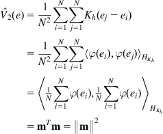 (4.64)
where ![]() is the mean vector of the data in kernel space.
is the mean vector of the data in kernel space.
In addition to the previous properties, the literature [102] points out that the empirical error entropy has the dilation feature, that is, as the kernel width ![]() increases, the performance surface (surface of the empirical error entropy in parameter space) will become more and more flat, thus leading to the local extrema reducing gradually and even disappearing. Figure 4.3 illustrates the contour plots of a two-dimensional performance surface of ADALINE parameter identification based on the order-
increases, the performance surface (surface of the empirical error entropy in parameter space) will become more and more flat, thus leading to the local extrema reducing gradually and even disappearing. Figure 4.3 illustrates the contour plots of a two-dimensional performance surface of ADALINE parameter identification based on the order-![]() IP criterion. It is clear to see that the IPs corresponding to different
IP criterion. It is clear to see that the IPs corresponding to different ![]() values all have the feature of dilation. The dilation feature implies that one can obtain desired performance surface by means of proper selection of the kernel width.
values all have the feature of dilation. The dilation feature implies that one can obtain desired performance surface by means of proper selection of the kernel width.

Figure 4.3 Contour plots of a two-dimensional performance surface of ADALINE parameter identification based on the order-![]() IP criterion (adopted from Ref. [102]).
IP criterion (adopted from Ref. [102]).
4.3 Identification Algorithms Under MEE Criterion
4.3.1 Nonparametric Information Gradient Algorithms
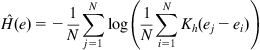
In general, information gradient (IG) algorithms refer to the gradient-based identification algorithms under MEE criterion (i.e., minimizing the empirical error entropy), including the batch information gradient (BIG) algorithm, sliding information gradient algorithm, forgetting recursive information gradient (FRIG) algorithm, and stochastic information gradient (SIG) algorithm. If the empirical error entropy is estimated by nonparametric approaches (like KDE), then they are called the nonparametric IG algorithms. In the following, we present several nonparametric IG algorithms that are based on ![]() -entropy and KDE.
-entropy and KDE.
4.3.1.1 BIG Algorithm
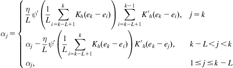
With the empirical ![]() -entropy as the criterion function, the BIG identification algorithm is derived as follows:
-entropy as the criterion function, the BIG identification algorithm is derived as follows:
 (4.65)
where ![]() is the step-size,
is the step-size, ![]() is the number of training data,
is the number of training data, ![]() and
and ![]() denote, respectively, the first-order derivatives of functions
denote, respectively, the first-order derivatives of functions ![]() and
and ![]() . The gradient
. The gradient ![]() of the model output with respect to the parameter
of the model output with respect to the parameter ![]() depends on the specific model structure. For example, if the model is an ADALINE or FIR filter, we have
depends on the specific model structure. For example, if the model is an ADALINE or FIR filter, we have ![]() . The reason for the algorithm named as the BIG algorithm is because that the empirical error entropy is calculated based on all the training data.
. The reason for the algorithm named as the BIG algorithm is because that the empirical error entropy is calculated based on all the training data.
Given a specific ![]() function, we obtain a specific algorithm:
function, we obtain a specific algorithm:


In above algorithms, if the kernel function is Gaussian function, the derivative ![]() will be
will be
![]() (4.68)
(4.68)
The step-size ![]() is a crucial parameter that controls the compromise between convergence speed and misadjustment, and has significant influence on the learning (identification) performance. In practical use, the selection of step-size should guarantees the stability and convergence rate of the algorithm. To further improve the performance, the step-size
is a crucial parameter that controls the compromise between convergence speed and misadjustment, and has significant influence on the learning (identification) performance. In practical use, the selection of step-size should guarantees the stability and convergence rate of the algorithm. To further improve the performance, the step-size ![]() can be designed as a variable step-size. In Ref. [105], a self-adjusting step-size (SAS) was proposed to improve the performance of QIP criterion, i.e.,
can be designed as a variable step-size. In Ref. [105], a self-adjusting step-size (SAS) was proposed to improve the performance of QIP criterion, i.e.,
![]() (4.69)
(4.69)
where ![]() and
and ![]() is a symmetric and unimodal kernel function (hence
is a symmetric and unimodal kernel function (hence ![]() ).
).
The kernel width ![]() is another important parameter that controls the smoothness of the performance surface. In general, the kernel width can be set manually or determined in advance by Silverman’s rule. To make the algorithm converge to the global solution, one can start the algorithm with a large kernel width and decrease this parameter slowly during the course of adaptation, just like in stochastic annealing. In Ref. [185], an adaptive kernel width was proposed to improve the performance.
is another important parameter that controls the smoothness of the performance surface. In general, the kernel width can be set manually or determined in advance by Silverman’s rule. To make the algorithm converge to the global solution, one can start the algorithm with a large kernel width and decrease this parameter slowly during the course of adaptation, just like in stochastic annealing. In Ref. [185], an adaptive kernel width was proposed to improve the performance.
The BIG algorithm needs to acquire in advance all the training data, and hence is not suitable for online identification. To address this issue, one can use the sliding information gradient algorithm.
4.3.1.2 Sliding Information Gradient Algorithm
The sliding information gradient algorithm utilizes a set of recent error samples to estimate the error entropy. Specifically, the error samples used to calculate the error entropy at time ![]() is as follows9 :
is as follows9 :
![]() (4.70)
(4.70)
where ![]() denotes the sliding data length (
denotes the sliding data length (![]() ). Then the error entropy at time
). Then the error entropy at time ![]() can be estimated as
can be estimated as
 (4.71)
And hence, the sliding information gradient algorithm can be derived as
 (4.72)
For the case ![]() (corresponding to QIP), the above algorithm becomes
(corresponding to QIP), the above algorithm becomes
![]() (4.73)
(4.73)
4.3.1.3 FRIG Algorithm
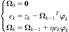
In the sliding information gradient algorithm, the error entropy can be estimated by a forgetting recursive method [64]. Assume at time ![]() the estimated error PDF is
the estimated error PDF is ![]() , then the error PDF at time
, then the error PDF at time ![]() can be estimated as
can be estimated as
![]() (4.74)
(4.74)
where ![]() is the forgetting factor. Therefore, we can calculate the empirical error entropy as follows:
is the forgetting factor. Therefore, we can calculate the empirical error entropy as follows:
 (4.75)
If ![]() (
(![]() ), there exists a recursive form [186]:
), there exists a recursive form [186]:
![]() (4.76)
(4.76)
where ![]() is the QIP at time
is the QIP at time ![]() . Thus, we have the following algorithm:
. Thus, we have the following algorithm:
 (4.77)
namely the FRIG algorithm. Compared with the sliding information gradient algorithm, the FRIG algorithm is computationally simpler and is more suitable for nonstationary system identification.
4.3.1.4 SIG Algorithm
In the empirical error entropy of (4.71), if dropping the outer averaging operator (![]() ), one may obtain the instantaneous error entropy at time
), one may obtain the instantaneous error entropy at time ![]() :
:
 (4.78)
The instantaneous error entropy is similar to the instantaneous error cost ![]() , as both are obtained by removing the expectation operator (or averaging operator) from the original criterion function. The computational cost of the instantaneous error entropy (4.78) is
, as both are obtained by removing the expectation operator (or averaging operator) from the original criterion function. The computational cost of the instantaneous error entropy (4.78) is ![]() of that of the empirical error entropy of Eq. (4.71). The gradient identification algorithm based on the instantaneous error entropy is called the SIG algorithm, which can be derived as
of that of the empirical error entropy of Eq. (4.71). The gradient identification algorithm based on the instantaneous error entropy is called the SIG algorithm, which can be derived as
 (4.79)
If ![]() , we obtain the SIG algorithm under Shannon entropy criterion:
, we obtain the SIG algorithm under Shannon entropy criterion:
 (4.80)
If ![]() , we get the SIG algorithm under QIP criterion:
, we get the SIG algorithm under QIP criterion:
![]() (4.81)
(4.81)
The SIG algorithm (4.81) is actually the FRIG algorithm with ![]() .
.
4.3.2 Parametric IG Algorithms
In IG algorithms described above, the error distribution is estimated by nonparametric KDE approach. With this approach, one is often confronted with the problem of how to choose a suitable value of the kernel width. An inappropriate choice of width will significantly deteriorate the performance of the algorithm. Though the effects of the kernel width on the shape of the performance surface and the eigenvalues of the Hessian at and around the optimal solution have been carefully investigated [102], at present the choice of the kernel width is still a difficult task. Thus, a certain parameterized density estimation, which does not involve the choice of kernel width, sometimes might be more practical. Especially, if some prior knowledge about the data distribution is available, the parameterized density estimation may achieve a better accuracy than nonparametric alternatives.
Next, we discuss the parametric IG algorithms that adopt parametric approaches to estimate the error distribution. To simplify the discussion, we only present the parametric SIG algorithm.
In general, the SIG algorithm can be expressed as
![]() (4.82)
(4.82)
where ![]() is the value of the error PDF at
is the value of the error PDF at ![]() estimated based on the error samples
estimated based on the error samples ![]() . By KDE approach, we have
. By KDE approach, we have
![]() (4.83)
(4.83)
Now we use a parametric approach to estimate ![]() . Let’s consider the exponential (maximum entropy) PDF form:
. Let’s consider the exponential (maximum entropy) PDF form:
 (4.84)
where the parameters ![]() (
(![]() ) can be estimated by some classical estimation methods like the ML estimation. After obtaining the estimated parameter values
) can be estimated by some classical estimation methods like the ML estimation. After obtaining the estimated parameter values ![]() , one can calculate
, one can calculate ![]() as
as
 (4.85)
Substituting Eq. (4.85) into Eq. (4.82), we obtain the following parametric SIG algorithm:
 (4.86)
If adopting Shannon entropy (![]() ), the algorithm becomes
), the algorithm becomes
 (4.87)
The selection of the PDF form is very important. Some typical PDF forms are as follows [187–190]:
where ![]() ,
, ![]() is the standard deviation, and
is the standard deviation, and ![]() is the Gamma function:
is the Gamma function:
![]() (4.89)
(4.89)
In the following, we present the SIG algorithm based on GGD model.
The GGD model has three parameters: location (mean) parameter ![]() , shape parameter
, shape parameter ![]() , and dispersion parameter
, and dispersion parameter ![]() . It has simple yet flexible functional forms and could approximate a large number of statistical distributions, and is widely used in image coding, speech recognition, and BSS, etc. The GGD densities include Gaussian (
. It has simple yet flexible functional forms and could approximate a large number of statistical distributions, and is widely used in image coding, speech recognition, and BSS, etc. The GGD densities include Gaussian (![]() ) and Laplace (
) and Laplace (![]() ) distributions as special cases. Figure 4.4 shows the GGD distributions for several shape parameters with zero mean and deviation
) distributions as special cases. Figure 4.4 shows the GGD distributions for several shape parameters with zero mean and deviation ![]() . It is evident that smaller values of the shape parameter correspond to heavier tails and therefore to sharper distributions. In the limiting cases, as
. It is evident that smaller values of the shape parameter correspond to heavier tails and therefore to sharper distributions. In the limiting cases, as ![]() , the GGD becomes close to the uniform distribution, whereas as
, the GGD becomes close to the uniform distribution, whereas as ![]() , it approaches an impulse function (
, it approaches an impulse function (![]() -distribution).
-distribution).

Utilizing the GGD model to estimate the error distribution is actually to estimate the parameters ![]() ,
, ![]() , and
, and ![]() based on the error samples. Up to now, there are many methods on how to estimate the GGD parameters [192]. Here, we only discuss the moment matching method (method of moments).
based on the error samples. Up to now, there are many methods on how to estimate the GGD parameters [192]. Here, we only discuss the moment matching method (method of moments).
The order-![]() absolute central moment of GGD distribution can be calculated as
absolute central moment of GGD distribution can be calculated as
![]() (4.90)
(4.90)
Hence we have
![]() (4.91)
(4.91)
The right-hand side of Eq. (4.91) is a function of ![]() , denoted by
, denoted by ![]() . Thus the parameter
. Thus the parameter ![]() can be expressed as
can be expressed as
![]() (4.92)
(4.92)
where ![]() is the inverse of function
is the inverse of function ![]() . Figure 4.5 shows the curves of the inverse function
. Figure 4.5 shows the curves of the inverse function ![]() when
when ![]() .
.

According to Eq. (4.92), based on the moment matching method one can estimate the parameters ![]() ,
, ![]() , and
, and ![]() as follows:
as follows:
 (4.93)
where the subscript ![]() represents that the values are estimated based on the error samples
represents that the values are estimated based on the error samples ![]() . Thus
. Thus ![]() will be
will be
 (4.94)
Substituting Eq. (4.94) into Eq. (4.82) and letting ![]() (Shannon entropy), we obtain the SIG algorithm based on GGD model:
(Shannon entropy), we obtain the SIG algorithm based on GGD model:
 (4.95)
where ![]() ,
, ![]() , and
, and ![]() are calculated by Eq. (4.93).
are calculated by Eq. (4.93).
To make a distinction, we denote “SIG-kernel” and “SIG-GGD” the SIG algorithms based on kernel approach and GGD densities, respectively. Compared with the SIG-kernel algorithm, the SIG-GGD just needs to estimate the three parameters of GGD density, without resorting to the choice of kernel width and the calculation of kernel function.
Comparing Eqs. (4.95) and (4.28), we find that when ![]() , the SIG-GGD algorithm can be considered as an LMP algorithm with adaptive order
, the SIG-GGD algorithm can be considered as an LMP algorithm with adaptive order ![]() and variable step-size
and variable step-size ![]() . In fact, under certain conditions, the SIG-GGD algorithm will converge to a certain LMP algorithm with fixed order and step-size. Consider the FIR system identification, in which the plant and the adaptive model are both FIR filters with the same order, and the additive noise
. In fact, under certain conditions, the SIG-GGD algorithm will converge to a certain LMP algorithm with fixed order and step-size. Consider the FIR system identification, in which the plant and the adaptive model are both FIR filters with the same order, and the additive noise ![]() is zero mean, ergodic, and stationary. When the model weight vector
is zero mean, ergodic, and stationary. When the model weight vector ![]() converges to the neighborhood of the plant weight vector
converges to the neighborhood of the plant weight vector ![]() , we have
, we have
![]() (4.96)
(4.96)
where ![]() is the weight error vector. In this case, the estimated values of the parameters in SIG-GGD algorithm will be
is the weight error vector. In this case, the estimated values of the parameters in SIG-GGD algorithm will be
 (4.97)
Since noise ![]() is an ergodic and stationary process, if
is an ergodic and stationary process, if ![]() is large enough, the estimated values of the three parameters will tend to some constants, and consequently, the SIG-GGD algorithm will converge to a certain LMP algorithm with fixed order and step-size. Clearly, if noise
is large enough, the estimated values of the three parameters will tend to some constants, and consequently, the SIG-GGD algorithm will converge to a certain LMP algorithm with fixed order and step-size. Clearly, if noise ![]() is Gaussian distributed, the SIG-GGD algorithm will converge to the LMS algorithm (
is Gaussian distributed, the SIG-GGD algorithm will converge to the LMS algorithm (![]() ), and if
), and if ![]() is Laplacian distributed, the algorithm will converge to the LAD algorithm (
is Laplacian distributed, the algorithm will converge to the LAD algorithm (![]() ). In Ref. [28], it has been shown that under slow adaptation, the LMS and LAD algorithms are, respectively, the optimum algorithms for the Gaussian and Laplace interfering noises. We may therefore conclude that the SIG-GGD algorithm has the ability to adjust its parameters so as to automatically switch to a certain optimum algorithm.
). In Ref. [28], it has been shown that under slow adaptation, the LMS and LAD algorithms are, respectively, the optimum algorithms for the Gaussian and Laplace interfering noises. We may therefore conclude that the SIG-GGD algorithm has the ability to adjust its parameters so as to automatically switch to a certain optimum algorithm.
There are two points that deserve special mention concerning the implementation of the SIG-GGD algorithm: (i) since there is no analytical expression, the calculation of the inverse function ![]() needs to use look-up table or some interpolation method and (ii) in order to avoid too large gradient and ensure the stability of the algorithm, it is necessary to set an upper bound on the parameter
needs to use look-up table or some interpolation method and (ii) in order to avoid too large gradient and ensure the stability of the algorithm, it is necessary to set an upper bound on the parameter ![]() .
.
4.3.3 Fixed-Point Minimum Error Entropy Algorithm
Given a mapping ![]() , the fixed points are solutions of iterative equation
, the fixed points are solutions of iterative equation ![]() ,
, ![]() . The fixed-point (FP) iteration is a numerical method of computing fixed points of iterated functions. Given an initial point
. The fixed-point (FP) iteration is a numerical method of computing fixed points of iterated functions. Given an initial point ![]() , the FP iteration algorithm is
, the FP iteration algorithm is
![]() (4.98)
(4.98)
where ![]() is the iterative index. If
is the iterative index. If ![]() is a function defined on the real line with real values, and is Lipschitz continuous with Lipschitz constant smaller than 1.0, then
is a function defined on the real line with real values, and is Lipschitz continuous with Lipschitz constant smaller than 1.0, then ![]() has precisely one fixed point, and the FP iteration converges toward that fixed point for any initial guess
has precisely one fixed point, and the FP iteration converges toward that fixed point for any initial guess ![]() . This result can be generalized to any metric space.
. This result can be generalized to any metric space.
The FP algorithm can be applied in parameter identification under MEE criterion [64]. Let’s consider the QIP criterion:
![]() (4.99)
(4.99)
under which the optimal parameter (weight vector) ![]() satisfies
satisfies
![]() (4.100)
(4.100)
If the model is an FIR filter, and the kernel function is the Gaussian function, we have
![]() (4.101)
(4.101)
One can write Eq. (4.101) in an FP iterative form (utilizing ![]() ):
):
 (4.102)
Then we have the following FP algorithm:
![]() (4.103)
(4.103)
where
 (4.104)
The above algorithm is called the fixed-point minimum error entropy (FP-MEE) algorithm. The FP-MEE algorithm can also be implemented by using the forgetting recursive form [194], i.e.,
![]() (4.105)
(4.105)
where
 (4.106)
This is the recursive fixed-point minimum error entropy (RFP-MEE) algorithm.
In addition to the parameter search algorithms described above, there are many other parameter search algorithms to minimize the error entropy. Several advanced parameter search algorithms are presented in Ref. [104], including the conjugate gradient (CG) algorithm, Levenberg–Marquardt (LM) algorithm, quasi-Newton method, and others.
4.3.4 Kernel Minimum Error Entropy Algorithm
System identification algorithms under MEE criterion can also be derived in kernel space. Existing KAF algorithms are mainly based on the MSE (or least squares) criterion. MSE is not always a suitable criterion especially in nonlinear and non-Gaussian situations. Hence, it is attractive to develop a new KAF algorithm based on a non-MSE (nonquadratic) criterion. In Ref. [139], a KAF algorithm under the maximum correntropy criterion (MCC), namely the kernel maximum correntropy (KMC) algorithm, has been developed. Similar to the KLMS, the KMC is also a stochastic gradient algorithm in RKHS. If the kernel function used in correntropy, denoted by ![]() , is the Gaussian kernel, the KMC algorithm can be derived as [139]
, is the Gaussian kernel, the KMC algorithm can be derived as [139]
![]() (4.107)
(4.107)
where ![]() denotes the estimated weight vector at iteration
denotes the estimated weight vector at iteration ![]() in a high-dimensional feature space
in a high-dimensional feature space ![]() induced by Mercer kernel
induced by Mercer kernel ![]() and
and ![]() is a feature vector obtained by transforming the input vector
is a feature vector obtained by transforming the input vector ![]() into the feature space through a nonlinear mapping
into the feature space through a nonlinear mapping ![]() . The KMC algorithm can be regarded as a KLMS algorithm with variable step-size
. The KMC algorithm can be regarded as a KLMS algorithm with variable step-size ![]() .
.
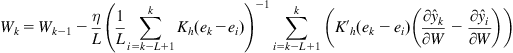
In the following, we will derive a KAF algorithm under the MEE criterion. Since the ![]() -entropy is a very general and flexible entropy definition, we use the
-entropy is a very general and flexible entropy definition, we use the ![]() -entropy of the error as the adaptation criterion. In addition, for simplicity we adopt the instantaneous error entropy (4.78) as the cost function. Then, one can easily derive the following kernel minimum error entropy (KMEE) algorithm:
-entropy of the error as the adaptation criterion. In addition, for simplicity we adopt the instantaneous error entropy (4.78) as the cost function. Then, one can easily derive the following kernel minimum error entropy (KMEE) algorithm:
 (4.108)
The KMEE algorithm (4.108) is actually the SIG algorithm in kernel space. By selecting a certain ![]() function, we can obtain a specific KMEE algorithm. For example, if setting
function, we can obtain a specific KMEE algorithm. For example, if setting ![]() (i.e.,
(i.e., ![]() ), we get the KMEE under Shannon entropy criterion:
), we get the KMEE under Shannon entropy criterion:
 (4.109)
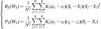
The weight update equation of Eq. (4.108) can be written in a compact form:
![]() (4.110)
(4.110)
where ![]() ,
, ![]() , and
, and ![]() is a vector-valued function of
is a vector-valued function of ![]() , expressed as
, expressed as
 (4.111)
The KMEE algorithm is similar to the KAPA [178], except that the error vector ![]() in KMEE is nonlinearly transformed by the function
in KMEE is nonlinearly transformed by the function ![]() . The learning rule of the KMEE in the original input space can be written as (
. The learning rule of the KMEE in the original input space can be written as (![]() )
)
![]() (4.112)
(4.112)
The learned model by KMEE has the same structure as that learned by KLMS, and can be represented as a linear combination of kernels centered in each data points:
![]() (4.113)
(4.113)
where the coefficients (at iteration ![]() ) are updated as follows:
) are updated as follows:
 (4.114)
The pseudocode for KMEE is summarized in Table 4.2.

4.3.5 Simulation Examples
In the following, we present several simulation examples to demonstrate the performance (accuracy, robustness, convergence rate, etc.) of the identification algorithms under MEE criterion.
Example 4.1 [102]
Assume that both the unknown system and the model are two-dimensional ADALINEs, i.e.,
![]() (4.115)
(4.115)
where unknown weight vector is ![]() , and
, and ![]() is the independent and zero-mean Gaussian noise. The goal is to identify the model parameters
is the independent and zero-mean Gaussian noise. The goal is to identify the model parameters ![]() under noises of different signal-to-noise ratios (SNRs). For each noise energy, 100 independent Monte-Carlo simulations are performed with
under noises of different signal-to-noise ratios (SNRs). For each noise energy, 100 independent Monte-Carlo simulations are performed with ![]() (
(![]() ) training data that are chosen randomly. In the simulation, the BIG algorithm under QIP criterion is used, and the kernel function
) training data that are chosen randomly. In the simulation, the BIG algorithm under QIP criterion is used, and the kernel function ![]() is the Gaussian function with bandwidth
is the Gaussian function with bandwidth ![]() . Figure 4.6 shows the average distance between actual and estimated optimal weight vector. For comparison purpose, the figure also includes the identification results (by solving the Wiener-Hopf equations) under MSE criterion. Simulation results indicate that, when SNR is higher (
. Figure 4.6 shows the average distance between actual and estimated optimal weight vector. For comparison purpose, the figure also includes the identification results (by solving the Wiener-Hopf equations) under MSE criterion. Simulation results indicate that, when SNR is higher (![]() ), the MEE criterion achieves much better accuracy than the MSE criterion (or requires less training data when achieving the same accuracy).
), the MEE criterion achieves much better accuracy than the MSE criterion (or requires less training data when achieving the same accuracy).
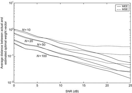
Figure 4.6 Comparison of the performance of MEE against MSE (adopted from Ref. [102]).
Example 4.2 [100]
Identify the following nonlinear dynamic system:
 (4.116)
where ![]() and
and ![]() are the state variables and
are the state variables and ![]() is the input signal. The identification model is the time delay neural network (TDNN), where the network structure is an MLP with multi-input, single hidden layer, and single output. The input vector of the neural network contains the current input and output and their past values of the nonlinear system, that is, the training data can be expressed as
is the input signal. The identification model is the time delay neural network (TDNN), where the network structure is an MLP with multi-input, single hidden layer, and single output. The input vector of the neural network contains the current input and output and their past values of the nonlinear system, that is, the training data can be expressed as
![]() (4.117)
(4.117)
In this example, ![]() and
and ![]() are set as
are set as ![]() . The number of hidden units is set at 7, and the symmetric sigmoid function is selected as the activation function. In addition, the number of training data is
. The number of hidden units is set at 7, and the symmetric sigmoid function is selected as the activation function. In addition, the number of training data is ![]() . We continue to compare the performance of MEE (using the BIG algorithm under QIP criterion) to MSE. For each criterion, the TDNN is trained starting from 50 different initial weight vectors, and the best solution (the one with the highest QIP or lowest MSE) among the 50 candidates is selected to test the performance.10 Figure 4.7 illustrates the probability densities of the error between system actual output and TDNN output with 10,000 testing data. One can see that the MEE criterion achieves a higher peak around the zero error. Figure 4.8 shows the probability densities of system actual output (desired output) and model output. Evidently, the output of the model trained under MEE criterion matches the desired output better.
. We continue to compare the performance of MEE (using the BIG algorithm under QIP criterion) to MSE. For each criterion, the TDNN is trained starting from 50 different initial weight vectors, and the best solution (the one with the highest QIP or lowest MSE) among the 50 candidates is selected to test the performance.10 Figure 4.7 illustrates the probability densities of the error between system actual output and TDNN output with 10,000 testing data. One can see that the MEE criterion achieves a higher peak around the zero error. Figure 4.8 shows the probability densities of system actual output (desired output) and model output. Evidently, the output of the model trained under MEE criterion matches the desired output better.
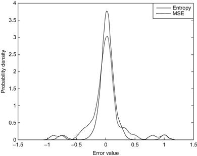
Figure 4.7 Probability densities of the error between system actual output and model output (adopted from Ref. [100]).

Figure 4.8 Probability densities of system actual output and model output (adopted from Ref. [100]).
Example 4.3 [190]
Compare the performances of SIG-kernel, SIG-GGD, and LMP family algorithms (LAD, LMS, LMF, etc.). Assume that both the unknown system and the model are FIR filters:
![]() (4.118)
(4.118)
where ![]() and
and ![]() denote the transfer functions of the system and the model, respectively. The initial weight vector of the model is set to be
denote the transfer functions of the system and the model, respectively. The initial weight vector of the model is set to be ![]() , and the input signal is white Gaussian noise with zero mean and unit power (variance). The kernel function in SIG-kernel algorithm is the Gaussian kernel with bandwidth determined by Silverman rule. In SIG-GGD algorithm, we set
, and the input signal is white Gaussian noise with zero mean and unit power (variance). The kernel function in SIG-kernel algorithm is the Gaussian kernel with bandwidth determined by Silverman rule. In SIG-GGD algorithm, we set ![]() , and to avoid large gradient, we set the upper bound of
, and to avoid large gradient, we set the upper bound of ![]() at 4.0.
at 4.0.
In the simulation, we consider four noise distributions (Laplace, Gaussian, Uniform, MixNorm), as shown in Figure 4.9. For each noise distribution, the average convergence curves, over 100 independent Monte Carlo simulations, are illustrated in Figure 4.10, where WEP denotes the weight error power, defined as
![]() (4.119)
(4.119)
where ![]() is the weight error vector (the difference between desired and estimated weight vectors) and
is the weight error vector (the difference between desired and estimated weight vectors) and ![]() is the weight error norm. Table 4.3 lists the average identification results (mean±deviation) of
is the weight error norm. Table 4.3 lists the average identification results (mean±deviation) of ![]() (
(![]() ). Further, the average evolution curves of
). Further, the average evolution curves of ![]() in SIG-GGD are shown in Figure 4.11.
in SIG-GGD are shown in Figure 4.11.
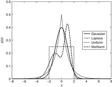
Figure 4.9 Four PDFs of the additive noise (adopted from Ref. [190]).

Figure 4.10 Average convergence curves of several algorithms for different noise distributions: (A) Laplace, (B) Gaussian, (C) Uniform, and (D) MixNorm (adopted from Ref. [190]).
Table 4.3
Average Identification Results of ![]() Over 100 Monte Carlo Simulations
Over 100 Monte Carlo Simulations

(adopted from Ref. [190])

Figure 4.11 Evolution curves of ![]() over 100 Monte Carlo runs: (A) Laplace, (B) Gaussian, and (C) Uniform (adopted from Ref. [190]).
over 100 Monte Carlo runs: (A) Laplace, (B) Gaussian, and (C) Uniform (adopted from Ref. [190]).
From the simulation results, we have the following observations:
i. The performances of LAD, LMS, and LMF depend crucially on the distribution of the disturbance noise. These algorithms may achieve the smallest misadjustment for a certain noise distribution (e.g., the LMF performs best in uniform noise); however, for other noise distributions, their performances may deteriorate dramatically (e.g., the LMF performs worst in Laplace noise).
ii. Both SIG-GGD and SIG-Kernel are robust to noise distribution. In the case of symmetric and unimodal noises (e.g., Laplace, Gaussian, Uniform), SIG-GGD may achieve a smaller misadjustment than SIG-Kernel. Though in the case of nonsymmetric and nonunimodal noises (e.g., MixNorm), SIG-GGD may be not as good as SIG-Kernel, it is still better than most of the LMP algorithms.
iii. Near the convergence, the parameter ![]() in SIG-GGD converges approximately to 1, 2, and 4 (note that
in SIG-GGD converges approximately to 1, 2, and 4 (note that ![]() is restricted to
is restricted to ![]() artificially) when disturbed by, respectively, Laplace, Gaussian, and Uniform noises. This confirms the fact that SIG-GGD has the ability to adjust its parameters so as to switch to a certain optimum algorithm.
artificially) when disturbed by, respectively, Laplace, Gaussian, and Uniform noises. This confirms the fact that SIG-GGD has the ability to adjust its parameters so as to switch to a certain optimum algorithm.
Example 4.4 [194]
Apply the RFP-MEE algorithm to identify the following FIR filter:
![]() (4.120)
(4.120)
The adaptive model is also an FIR filter with equal order. The input to both the plant and adaptive model is white Gaussian noise with unit power. The observation noise is white Gaussian distributed with zero mean and variance ![]() . The main objective is to investigate the effect of the forgetting factor on the convergence speed and convergence accuracy (WEP after convergence) of the RFP-MEE algorithm. Figure 4.12 shows the convergence curves of the RFP-MEE with different forgetting factors. One can see that smaller forgetting factors result in faster convergence speed and larger steady-state WEP. This result conforms to the well-known general behavior of the forgetting factor in recursive estimates. Thus, selecting a proper forgetting factor for RFP-MEE must consider the intrinsic trade-off between convergence speed and identification accuracy.
. The main objective is to investigate the effect of the forgetting factor on the convergence speed and convergence accuracy (WEP after convergence) of the RFP-MEE algorithm. Figure 4.12 shows the convergence curves of the RFP-MEE with different forgetting factors. One can see that smaller forgetting factors result in faster convergence speed and larger steady-state WEP. This result conforms to the well-known general behavior of the forgetting factor in recursive estimates. Thus, selecting a proper forgetting factor for RFP-MEE must consider the intrinsic trade-off between convergence speed and identification accuracy.

Figure 4.12 Convergence curves of RFP-MEE algorithm with different forgetting factors (adopted from Ref. [194]).
Example 4.5
This example aims to demonstrate the performance of KMEE (with Shannon entropy or QIP criterion). For comparison purpose, we also show the performances of several other KAF algorithms: KLMS, KMC, and KAPA. Let’s consider the nonlinear system identification, where the nonlinear system is as follows [195]:
 (4.121)
The noise ![]() is of symmetric
is of symmetric ![]() -stable (
-stable (![]() ) distribution with characteristic function
) distribution with characteristic function
![]() (4.122)
(4.122)
where ![]() ,
, ![]() . When
. When ![]() , the distribution is a zero-mean Gaussian distribution with variance 0.01; while when
, the distribution is a zero-mean Gaussian distribution with variance 0.01; while when ![]() , the distribution corresponds to an impulsive noise with infinite variance.
, the distribution corresponds to an impulsive noise with infinite variance.
Figure 4.13 illustrates the average learning curves (over 200 Monte Carlo runs) for different ![]() values and Table 4.4 lists the testing MSE at final iteration. In the simulation, 1000 samples are used for training and another 100 clean samples are used for testing (the filter is fixed during the testing phase). Further, all the kernels (kernel of RKHS, kernel of correntropy, and kernel for density estimation) are selected to be the Gaussian kernel. The kernel parameter for RKHS is set at
values and Table 4.4 lists the testing MSE at final iteration. In the simulation, 1000 samples are used for training and another 100 clean samples are used for testing (the filter is fixed during the testing phase). Further, all the kernels (kernel of RKHS, kernel of correntropy, and kernel for density estimation) are selected to be the Gaussian kernel. The kernel parameter for RKHS is set at ![]() , kernel size for correntropy is
, kernel size for correntropy is ![]() , and kernel bandwidth for density estimation is
, and kernel bandwidth for density estimation is ![]() . The sliding data lengths for KMEE and KAPA are both set at
. The sliding data lengths for KMEE and KAPA are both set at ![]() . The step-sizes for KLMS, KMC, KAPA, KMEE (Shannon), and KMEE (QIP), are, respectively, set at 0.8, 1.0, 0.05, 1.0, and 2.0. These parameters are experimentally selected to achieve the desirable performance. From Figure 4.13 and Table 4.4, one can see that the KMEE algorithms outperform all other algorithms except for the case of small
. The step-sizes for KLMS, KMC, KAPA, KMEE (Shannon), and KMEE (QIP), are, respectively, set at 0.8, 1.0, 0.05, 1.0, and 2.0. These parameters are experimentally selected to achieve the desirable performance. From Figure 4.13 and Table 4.4, one can see that the KMEE algorithms outperform all other algorithms except for the case of small ![]() , the KMC algorithm may achieve a relatively smaller deviation in testing MSE. Simulation results also show that the performances of KMEE (Shannon) and KMEE (QIP) are very close.
, the KMC algorithm may achieve a relatively smaller deviation in testing MSE. Simulation results also show that the performances of KMEE (Shannon) and KMEE (QIP) are very close.


4.4 Convergence Analysis
Next, we analyze the convergence properties of the parameter identification under MEE criterion. For simplicity, we consider only the ADALINE model (which includes the FIR filter as a special case). The convergence analysis of error entropy minimization algorithms is, in general, rather complicated. This is mostly because
1. the objective function (the empirical error entropy) is not only related to the current error but also concerned with the past error values;
2. the entropy function and the kernel function are nonlinear functions;
3. the shape of performance surface is very complex (nonquadratic and nonconvex).
There are two ways for the convergence analysis of such algorithms: (i) using the Taylor series expansion near the optimal solution to obtain an approximate linearization algorithm, and then performing the convergence analysis for the linearization algorithm and (ii) applying the energy conservation relation to analyze the convergence behavior [106]. The first approach is relatively simple, but only the approximate analysis results near the optimal solution can be achieved. With the second approach it is possible to acquire rigorous analysis results of the convergence, but usually more assumptions are needed. In the following, we first briefly introduce the first analysis approach, and then focus on the second approach, performing the mean square convergence analysis based on the energy conservation relation. The following analysis is mainly aimed at the nonparametric IG algorithms with KDE.
4.4.1 Convergence Analysis Based on Approximate Linearization
In Ref. [102], an approximate linearization approach has been used to analyze the convergence of the gradient-based algorithm under order-![]() IP criterion. Consider the ADALINE model:
IP criterion. Consider the ADALINE model:
![]() (4.123)
(4.123)
where ![]() is the
is the ![]() -dimensional input vector,
-dimensional input vector, ![]() is the weight vector. The gradient based identification algorithm under order-
is the weight vector. The gradient based identification algorithm under order-![]() (
(![]() ) information potential criterion can be expressed as
) information potential criterion can be expressed as
![]() (4.124)
(4.124)
where ![]() denotes the gradient of the empirical order-
denotes the gradient of the empirical order-![]() IP with respect to the weight vector, which can be calculated as
IP with respect to the weight vector, which can be calculated as
 (4.125)
As the kernel function ![]() satisfies
satisfies ![]() , we have
, we have
![]() (4.126)
(4.126)
So, one can rewrite Eq. (4.125) as
 (4.127)
where ![]() .
.
If the weight vector ![]() lies in the neighborhood of the optimal solution
lies in the neighborhood of the optimal solution ![]() , one can obtain a linear approximation of the gradient
, one can obtain a linear approximation of the gradient ![]() using the first-order Taylor expansion:
using the first-order Taylor expansion:
![]() (4.128)
(4.128)
where ![]() is the Hessian matrix, i.e.,
is the Hessian matrix, i.e.,
 (4.129)
Substituting Eq. (4.128) into Eq. (4.124), and subtracting ![]() from both sides, one obtains
from both sides, one obtains
![]() (4.130)
(4.130)
where ![]() is the weight error vector. The convergence analysis of the above linear recursive algorithm is very simple. Actually, one can just borrow the well-known convergence analysis results from the LMS convergence theory [18–20]. Assume that the Hessian matrix
is the weight error vector. The convergence analysis of the above linear recursive algorithm is very simple. Actually, one can just borrow the well-known convergence analysis results from the LMS convergence theory [18–20]. Assume that the Hessian matrix ![]() is a normal matrix and can be decomposed into the following normal form:
is a normal matrix and can be decomposed into the following normal form:
![]() (4.131)
(4.131)
where ![]() is an
is an ![]() orthogonal matrix,
orthogonal matrix, ![]() ,
, ![]() is the eigenvalue of
is the eigenvalue of ![]() . Then, the linear recursion (4.130) can be expressed as
. Then, the linear recursion (4.130) can be expressed as
![]() (4.132)
(4.132)
Clearly, if the following conditions are satisfied, the weight error vector ![]() will converge to the zero vector (or equivalently, the weight vector
will converge to the zero vector (or equivalently, the weight vector ![]() will converge to the optimal solution):
will converge to the optimal solution):
![]() (4.133)
(4.133)
Thus, a sufficient condition that ensures the convergence of the algorithm is
 (4.134)
Further, the approximate time constant corresponding to ![]() will be
will be
![]() (4.135)
(4.135)
In Ref. [102], it has also been proved that if the kernel width ![]() increases, the absolute values of the eigenvalues will decrease, and the time constants will increase, that is, the convergence speed of the algorithm will become slower.
increases, the absolute values of the eigenvalues will decrease, and the time constants will increase, that is, the convergence speed of the algorithm will become slower.
4.4.2 Energy Conservation Relation
Here, the energy conservation relation is not the well-known physical law of conservation of energy, but refers to a certain identical relation that exists among the WEP, a priori error, and a posteriori error in adaptive filtering algorithms (such as the LMS algorithm). This fundamental relation can be used to analyze the mean square convergence behavior of an adaptive filtering algorithm [196].
Given an adaptive filtering algorithm with error nonlinearity [29]:
![]() (4.136)
(4.136)
where ![]() is the error nonlinearity function (
is the error nonlinearity function (![]() corresponds to the LMS algorithm), the following energy conservation relation holds:
corresponds to the LMS algorithm), the following energy conservation relation holds:
 (4.137)
where ![]() is the WEP at instant
is the WEP at instant ![]() (or iteration
(or iteration ![]() ),
), ![]() and
and ![]() are, respectively, the a priori error and a posteriori error:
are, respectively, the a priori error and a posteriori error:
![]() (4.138)
(4.138)
One can show that the IG algorithms (assuming ADALINE model) also satisfy the energy conservation relation similar to Eq. (4.137) [106]. Let us consider the sliding information gradient algorithm (with ![]() entropy criterion):
entropy criterion):
![]() (4.139)
(4.139)
where ![]() is the empirical error entropy at iteration
is the empirical error entropy at iteration ![]() :
:
 (4.140)
where ![]() ,
, ![]() is the
is the ![]() th error sample used to calculate the empirical error entropy at iteration
th error sample used to calculate the empirical error entropy at iteration ![]() . Given the
. Given the ![]() -function and the kernel function
-function and the kernel function ![]() , the empirical error entropy
, the empirical error entropy ![]() will be a function of the error vector
will be a function of the error vector ![]() , which can be written as
, which can be written as
![]() (4.141)
(4.141)
This function will be continuously differentiable with respect to ![]() , provided that both functions
, provided that both functions ![]() and
and ![]() are continuously differentiable.
are continuously differentiable.
In ADALINE system identification, the error ![]() will be
will be
![]() (4.142)
(4.142)
where ![]() is the
is the ![]() th measurement at iteration
th measurement at iteration ![]() ,
, ![]() is the
is the ![]() th model output at iteration
th model output at iteration ![]() ,
, ![]() is the
is the ![]() th input vector11 at iteration
th input vector11 at iteration ![]() , and
, and ![]() is the ADALINE weight vector. One can write Eq. (4.142) in the form of block data, i.e.,
is the ADALINE weight vector. One can write Eq. (4.142) in the form of block data, i.e.,
![]() (4.143)
(4.143)
where ![]() ,
, ![]() , and
, and ![]() (
(![]() input matrix).
input matrix).
The block data ![]() can be constructed in various manners. Two typical examples are
can be constructed in various manners. Two typical examples are


Combining Eqs. (4.139), (4.141), and (4.143), we can derive (assuming ADALINE model)
 (4.146)
where ![]() , in which
, in which
![]() (4.147)
(4.147)
With QIP criterion (![]() ), the function
), the function ![]() can be calculated as (assuming
can be calculated as (assuming ![]() is a Gaussian kernel):
is a Gaussian kernel):
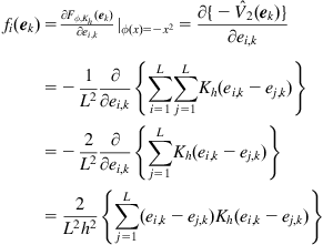 (4.148)
The algorithm in Eq. (4.146) is in form very similar to the adaptive filtering algorithm with error nonlinearity, as expressed in Eq. (4.136). In fact, Eq. (4.146) can be regarded, to some extent, as a “block” version of Eq. (4.136). Thus, one can study the mean square convergence behavior of the algorithm (4.146) by similar approach as in mean square analysis of the algorithm (4.136). It should also be noted that the objective function behind algorithm (4.146) is not limited to the error entropy. Actually, the cost function ![]() can be extended to any function of
can be extended to any function of ![]() , including the simple block mean square error (BMSE) criterion that is given by [197]
, including the simple block mean square error (BMSE) criterion that is given by [197]
![]() (4.149)
(4.149)
We now derive the energy conservation relation for the algorithm (4.146). Assume that the unknown system and the adaptive model are both ADALINE structures with the same dimension of weights.12 Let the measured output (in the form of block data) be
![]() (4.150)
(4.150)
where ![]() is the weight vector of unknown system and
is the weight vector of unknown system and ![]() is the noise vector. In this case, the error vector
is the noise vector. In this case, the error vector ![]() can be expressed as
can be expressed as
![]() (4.151)
(4.151)
where ![]() is the weight error vector. In addition, we define the a priori and a posteriori error vectors
is the weight error vector. In addition, we define the a priori and a posteriori error vectors ![]() and
and ![]() :
:
 (4.152)
Clearly, ![]() and
and ![]() have the following relationship:
have the following relationship:
![]() (4.153)
(4.153)
Combining Eqs. (4.146) and (4.153) yields
![]() (4.154)
(4.154)
where ![]() is an
is an ![]() symmetric matrix with elements
symmetric matrix with elements ![]() .
.
Assume that the matrix ![]() is invertible (i.e.,
is invertible (i.e., ![]() ). Then we have
). Then we have
![]() (4.155)
(4.155)
And hence
![]() (4.156)
(4.156)
Both sides of Eq. (4.156) should have the same energy, i.e.,
![]() (4.157)
(4.157)
From Eq. (4.157), after some simple manipulations, we obtain the following energy conservation relation:
![]() (4.158)
(4.158)
where ![]() ,
, ![]() ,
, ![]() . Further, in order to analyze the mean square convergence performance of the algorithm, we take the expectations of both sides of (4.158) and write
. Further, in order to analyze the mean square convergence performance of the algorithm, we take the expectations of both sides of (4.158) and write
![]() (4.159)
(4.159)
The energy conservation relation (4.159) shows how the energies (powers) of the error quantities evolve in time, which is exact for any adaptive algorithm described in Eq. (4.146), and is derived without any approximation and assumption (except for the condition that ![]() is invertible). One can also observe that Eq. (4.159) is a generalization of Eq. (4.137) in the sense that the a priori and a posteriori error quantities are extended to vector case.
is invertible). One can also observe that Eq. (4.159) is a generalization of Eq. (4.137) in the sense that the a priori and a posteriori error quantities are extended to vector case.
4.4.3 Mean Square Convergence Analysis Based on Energy Conservation Relation
The energy conservation relation (4.159) characterizes the evolution behavior of the weight error power (WEP). Substituting ![]() into (4.159), we obtain
into (4.159), we obtain
![]() (4.160)
(4.160)
To evaluate the expectations ![]() and
and ![]() , some assumptions are given below [106]:
, some assumptions are given below [106]:
• A1: The noise ![]() is independent, identically distributed, and independent of the input
is independent, identically distributed, and independent of the input ![]() ;
;
• A2: The a priori error vector ![]() is jointly Gaussian distributed;
is jointly Gaussian distributed;
• A3: The input vectors ![]() are zero-mean independent, identically distributed;
are zero-mean independent, identically distributed;
Remark:
Assumptions A1 and A2 are popular and have been widely used in convergence analysis for many adaptive filtering algorithms [196]. As pointed out in [29], the assumption A2 is reasonable for longer weight vector by central limit theorem arguments. The assumption A3 restricts the input sequence ![]() to white regression data, which is also a common practice in the literature (e.g., as in Refs. [28,198,199]). The assumption A4 is somewhat similar to the uncorrelation assumption in Ref. [29], but it is a little stronger. This assumption is reasonable under assumptions A1 and A3, and will become more realistic as the weight vector gets longer (justified by the law of large numbers).
to white regression data, which is also a common practice in the literature (e.g., as in Refs. [28,198,199]). The assumption A4 is somewhat similar to the uncorrelation assumption in Ref. [29], but it is a little stronger. This assumption is reasonable under assumptions A1 and A3, and will become more realistic as the weight vector gets longer (justified by the law of large numbers).
In the following, for tractability, we only consider the case in which the block data are constructed by “![]() -time shift” approach (see Eq. (4.145)). In this case, the assumption A3 implies: (i) the input matrices
-time shift” approach (see Eq. (4.145)). In this case, the assumption A3 implies: (i) the input matrices ![]() are zero-mean, independent, identically distributed and (ii)
are zero-mean, independent, identically distributed and (ii) ![]() and
and ![]() are mutually independent. Combining assumption A3 and the independence between
are mutually independent. Combining assumption A3 and the independence between ![]() and
and ![]() , one may easily conclude that the components of the a priori error vector
, one may easily conclude that the components of the a priori error vector ![]() are also zero-mean, independent, identically distributed. Thus, by Gaussian assumption A2, the PDF of
are also zero-mean, independent, identically distributed. Thus, by Gaussian assumption A2, the PDF of ![]() can be expressed as
can be expressed as
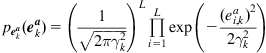 (4.161)
where ![]() is the a priori error power. Further, by assumption A1, the a priori error vector
is the a priori error power. Further, by assumption A1, the a priori error vector ![]() and the noise vector
and the noise vector ![]() are independent, and hence
are independent, and hence
 (4.162)
where ![]() denotes the PDF of
denotes the PDF of ![]() . The inner integral depends on
. The inner integral depends on ![]() through the second moment
through the second moment ![]() only, and so does
only, and so does ![]() . Thus, given the noise distribution
. Thus, given the noise distribution ![]() , the expectation
, the expectation ![]() can be expressed as a function of
can be expressed as a function of ![]() , which enables us to define the following function13 :
, which enables us to define the following function13 :
![]() (4.163)
(4.163)
It follows that
![]() (4.164)
(4.164)
Next, we evaluate the expectation ![]() . As
. As ![]() ,
, ![]() , by assumptions A1, A3, and A4,
, by assumptions A1, A3, and A4, ![]() and
and ![]() will be independent. Thus
will be independent. Thus
 (4.165)
where (a) and (b) follow from the assumption A3. Since ![]() is Gaussian and independent of the noise vector
is Gaussian and independent of the noise vector ![]() , the term
, the term ![]() will also depend on
will also depend on ![]() through
through ![]() only, and this prompts us to define the function
only, and this prompts us to define the function ![]() :
:
![]() (4.166)
(4.166)
Combining Eqs. (4.165) and (4.166) yields
![]() (4.167)
(4.167)
Substituting Eqs. (4.164) and (4.167) into Eq. (4.160), we obtain
![]() (4.168)
(4.168)
Now, we use the recursion formula (4.168) to analyze the mean square convergence behavior of the algorithm (4.146), following the similar derivations in Ref. [29].
4.4.3.1 Sufficient Condition for Mean Square Convergence
From Eq. (4.168), it is easy to observe
 (4.169)
Therefore, if we choose the step-size ![]() such that for all
such that for all ![]()
 (4.170)
then the sequence of WEP ![]() will be monotonically decreasing (and hence convergent). Thus, a sufficient condition for the mean square convergence of the algorithm (4.146) would be
will be monotonically decreasing (and hence convergent). Thus, a sufficient condition for the mean square convergence of the algorithm (4.146) would be
 (4.171)
where (a) comes from the assumption that the input vector is stationary, ![]() ,
, ![]() denotes the set of all possible values of
denotes the set of all possible values of ![]() (
(![]() ).
).
In general, the above upper bound of the step-size is conservative. However, if ![]() is a monotonically increasing function over
is a monotonically increasing function over ![]() , i.e.,
, i.e., ![]() ,
, ![]() , one can explicitly derive the maximum value (tight upper bound) of the step-size that ensures the mean square convergence. Let’s come back to the condition in Eq. (4.170) and write
, one can explicitly derive the maximum value (tight upper bound) of the step-size that ensures the mean square convergence. Let’s come back to the condition in Eq. (4.170) and write
![]() (4.172)
(4.172)
Under this condition, the WEP will be monotonically decreasing. As the a priori error power ![]() is proportional to the WEP
is proportional to the WEP ![]() (see Eq. (4.177)), in this case, the a priori error power will also be monotonically decreasing, i.e.,
(see Eq. (4.177)), in this case, the a priori error power will also be monotonically decreasing, i.e.,
![]() (4.173)
(4.173)
where ![]() is the initial a priori error power. So, the maximum step-size is
is the initial a priori error power. So, the maximum step-size is
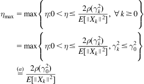 (4.174)
where (a) follows from Eq. (4.173) and the monotonic property of ![]() . This maximum step-size depends upon the initial a priori error power. When
. This maximum step-size depends upon the initial a priori error power. When ![]() , we have
, we have
 (4.175)
In this case, the learning is at the edge of convergence (WEP remains constant).
Remark
If the step-size ![]() is below the upper bound or smaller than the maximum value
is below the upper bound or smaller than the maximum value ![]() , the WEP will be decreasing. However, this does not imply that the WEP will converge to zero. There are two reasons for this. First, for a stochastic gradient-based algorithm, there always exist some excess errors (misadjustments). Second, the algorithm may converge to a local minimum (if any).
, the WEP will be decreasing. However, this does not imply that the WEP will converge to zero. There are two reasons for this. First, for a stochastic gradient-based algorithm, there always exist some excess errors (misadjustments). Second, the algorithm may converge to a local minimum (if any).
4.4.3.2 Mean Square Convergence Curve
One can establish a more homogeneous form for the recursion formula (4.168). First, it is easy to derive
 (4.176)
where (a) follows from the independence between ![]() and
and ![]() ,
, ![]() ,
, ![]() . As the input data are assumed to be zero-mean, independent, identically distributed, we have
. As the input data are assumed to be zero-mean, independent, identically distributed, we have ![]() (
(![]() is an
is an ![]() -dimensional unit matrix), and hence
-dimensional unit matrix), and hence
![]() (4.177)
(4.177)
Substituting Eq. (4.177) and ![]() into Eq. (4.168) yields the equation that governs the mean square convergence curve:
into Eq. (4.168) yields the equation that governs the mean square convergence curve:
![]() (4.178)
(4.178)
4.4.3.3 Mean Square Steady-State Performance
We can use Eq. (4.178) to evaluate the mean square steady-state performance. Suppose the WEP reaches a steady-state value, i.e.,
![]() (4.179)
(4.179)
Then the mean square convergence equation (4.178) becomes, in the limit
![]() (4.180)
(4.180)
It follows that
![]() (4.181)
(4.181)
Denote ![]() the steady-state WEP, i.e.,
the steady-state WEP, i.e., ![]() , we have
, we have
![]() (4.182)
(4.182)
Therefore, if the adaptive algorithm (4.146) converges, the steady-state WEP ![]() will be a positive solution of Eq. (4.182), or equivalently,
will be a positive solution of Eq. (4.182), or equivalently, ![]() will be a positive FP of the function
will be a positive FP of the function ![]() .
.
Further, denote ![]() the steady-state excess mean square error (EMSE), i.e.,
the steady-state excess mean square error (EMSE), i.e., ![]() . By Eq. (4.177), we can easily evaluate
. By Eq. (4.177), we can easily evaluate ![]() as
as
![]() (4.183)
(4.183)
The steady-state EMSE is in linear proportion to the steady-state WEP.
So far we have derived the mean square convergence performance for adaptive algorithm (4.146), under the assumptions A1–A4. The derived results depend mainly on two functions: ![]() ,
, ![]() . In the following, we will derive the exact expressions for the two functions for QIP criterion (
. In the following, we will derive the exact expressions for the two functions for QIP criterion (![]() ).
).
By Eq. (4.148), under QIP criterion we have
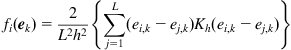 (4.184)
Hence, the function ![]() can be expressed as
can be expressed as
 (4.185)
where (a) comes from the fact that the error pairs ![]() are independent, identically distributed. In addition, substituting (4.184) into (4.166) yields
are independent, identically distributed. In addition, substituting (4.184) into (4.166) yields
 (4.186)
where (b) and (c) follow from the fact that the error samples ![]() are independent, identically distributed.
are independent, identically distributed.
In (4.185) and (4.186), the functions ![]() and
and ![]() do not yet have the explicit expressions in terms of the argument
do not yet have the explicit expressions in terms of the argument ![]() . In order to obtain the explicit expressions, one has to calculate the involved expectations using the PDFs of the a priori error and the noise. The calculation is rather complex and tedious. In the following, we only present the results for the Gaussian noise case.
. In order to obtain the explicit expressions, one has to calculate the involved expectations using the PDFs of the a priori error and the noise. The calculation is rather complex and tedious. In the following, we only present the results for the Gaussian noise case.
Let the noise ![]() be a zero-mean white Gaussian process with variance
be a zero-mean white Gaussian process with variance ![]() . Then the error
. Then the error ![]() will also be zero-mean Gaussian distributed with variance
will also be zero-mean Gaussian distributed with variance ![]() . In this case, one can derive
. In this case, one can derive
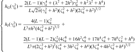 (4.187)
Substituting the explicit expressions in Eq. (4.187) into Eq. (4.178), one may obtain the exact convergence curve of the WEP, which can be described by a nonlinear dynamic system:
![]() (4.188)
(4.188)
where the function ![]() .
.
In the following, a Monte Carlo simulation example is presented to verify the previous theoretical analysis results [106]. Consider the case in which the input signal and additive noise are both white Gaussian processes with unit power. Assume the unknown and adaptive systems are both ADALINE structures with weight vector of length 25. The initial weight vector of the adaptive system was obtained by perturbing each coefficient of the ideal weight vector ![]() by a random variable that is zero-mean Gaussian distributed with variance 0.04 (hence the initial WEP is 1.0 or 0 dB).
by a random variable that is zero-mean Gaussian distributed with variance 0.04 (hence the initial WEP is 1.0 or 0 dB).
First, we examine the mean square convergence curves of the adaptive algorithm. For different values of the step-size ![]() , kernel width
, kernel width ![]() , and sliding data length
, and sliding data length ![]() , the average convergence curves (solid) over 100 Monte Carlo runs and the corresponding theoretical learning curves (dotted) are plotted in Figures 4.14–4.16. Clearly, the experimental and theoretical results agree very well. Second, we verify the steady-state performance. As shown in Figures 4.17–4.19, the steady-state EMSEs generated by simulations match well with those calculated by theory. These simulated and theoretical results also demonstrate how the step-size
, the average convergence curves (solid) over 100 Monte Carlo runs and the corresponding theoretical learning curves (dotted) are plotted in Figures 4.14–4.16. Clearly, the experimental and theoretical results agree very well. Second, we verify the steady-state performance. As shown in Figures 4.17–4.19, the steady-state EMSEs generated by simulations match well with those calculated by theory. These simulated and theoretical results also demonstrate how the step-size ![]() , kernel width
, kernel width ![]() , and sliding data length
, and sliding data length ![]() affect the performance of the adaptation: (i) a larger step-size produces a faster initial convergence, but results in a larger misadjustment; (ii) a larger kernel width causes a slower initial convergence, but yields a smaller misadjustment; (iii) a larger sliding data length achieves a faster initial convergence and a smaller misadjustment.14
affect the performance of the adaptation: (i) a larger step-size produces a faster initial convergence, but results in a larger misadjustment; (ii) a larger kernel width causes a slower initial convergence, but yields a smaller misadjustment; (iii) a larger sliding data length achieves a faster initial convergence and a smaller misadjustment.14
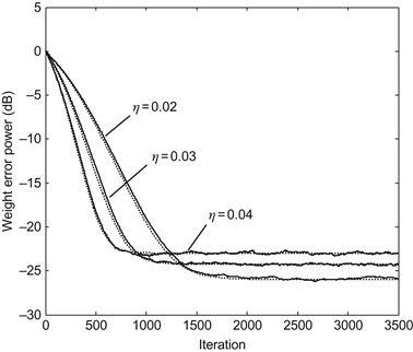


In addition, we verify the upper bound on step-sizes that guarantee the convergence of the learning. For the case in which the kernel width ![]() , and the sliding data length
, and the sliding data length ![]() , we plot in Figure 4.20 the curve of the function
, we plot in Figure 4.20 the curve of the function ![]() . Clearly, this function is monotonically increasing. Thus by (4.174), we can calculate the maximum step-size
. Clearly, this function is monotonically increasing. Thus by (4.174), we can calculate the maximum step-size ![]() . For step-sizes around
. For step-sizes around ![]() the simulated and theoretical learning curves are shown in Figure 4.21. As expected, when
the simulated and theoretical learning curves are shown in Figure 4.21. As expected, when ![]() , the learning is at the edge of convergence. If
, the learning is at the edge of convergence. If ![]() is above (or below) the maximum step-size
is above (or below) the maximum step-size ![]() , the weight error power will be increasing (or decreasing).
, the weight error power will be increasing (or decreasing).
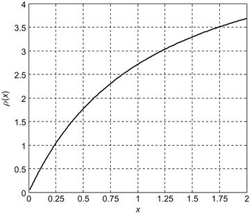

4.5 Optimization of  -Entropy Criterion
The ![]() -entropy criterion is very flexible. In fact, many entropy definitions are special cases of the
-entropy criterion is very flexible. In fact, many entropy definitions are special cases of the ![]() -entropy. This flexibility, however, also brings the problem of how to select a good
-entropy. This flexibility, however, also brings the problem of how to select a good ![]() function to maximize the performance of the adaptation algorithm [200].
function to maximize the performance of the adaptation algorithm [200].
The selection of the ![]() function is actually an optimization problem. Denote
function is actually an optimization problem. Denote ![]() a quantitative performance index (convergence speed, steady-state accuracy, etc.) of the algorithm that we would like to optimize. Then the optimal
a quantitative performance index (convergence speed, steady-state accuracy, etc.) of the algorithm that we would like to optimize. Then the optimal ![]() function will be
function will be
![]() (4.189)
(4.189)
where ![]() represents the set of all possible
represents the set of all possible ![]() functions. Due to the fact that different identification scenarios usually adopt different performance indexes, the above optimization problem must be further formulated in response to a specific identification system. In the following, we will focus on the FIR system identification, and assume for simplicity that the unknown system and the adaptive model are both FIR filters of the same order.
functions. Due to the fact that different identification scenarios usually adopt different performance indexes, the above optimization problem must be further formulated in response to a specific identification system. In the following, we will focus on the FIR system identification, and assume for simplicity that the unknown system and the adaptive model are both FIR filters of the same order.
Before proceeding, we briefly review the optimization of the general error criterion ![]() . In the adaptive filtering literature, there are mainly two approaches for the optimization of the general (usually non-MSE) error criterion. One approach regards the choice of the error criterion (or the
. In the adaptive filtering literature, there are mainly two approaches for the optimization of the general (usually non-MSE) error criterion. One approach regards the choice of the error criterion (or the ![]() function) as a parameter search, in which a suitable structure of the criterion is assumed [26,201]. Such a design method usually leads to a suboptimal algorithm since the criterion is limited to a restricted class of functions. Another approach is proposed by Douglas and Meng [28], where the calculus of variations is used, and no prior information about the structure of error criterion is assumed. According to Douglas’ method, in FIR system identification one can use the following performance index to optimize the error criterion:
function) as a parameter search, in which a suitable structure of the criterion is assumed [26,201]. Such a design method usually leads to a suboptimal algorithm since the criterion is limited to a restricted class of functions. Another approach is proposed by Douglas and Meng [28], where the calculus of variations is used, and no prior information about the structure of error criterion is assumed. According to Douglas’ method, in FIR system identification one can use the following performance index to optimize the error criterion:
![]() (4.190)
(4.190)
where ![]() is the weight error vector at
is the weight error vector at ![]() iteration. With the above performance index, the optimization of the
iteration. With the above performance index, the optimization of the ![]() function can be formulated as the following optimization problem [28]:
function can be formulated as the following optimization problem [28]:
 (4.191)
where ![]() ,
, ![]() is the error PDF at
is the error PDF at ![]() iteration,
iteration, ![]() is the step-size, and
is the step-size, and ![]() is the input signal power. By calculus of variations, one can obtain the optimal
is the input signal power. By calculus of variations, one can obtain the optimal ![]() function [28]:
function [28]:
![]() (4.192)
(4.192)
The optimal ![]() function can thus be expressed in the form of indefinite integral:
function can thus be expressed in the form of indefinite integral:
![]() (4.193)
(4.193)
which depends crucially on the error PDF ![]() .
.
Next, we will utilize Eq. (4.193) to derive an optimal ![]() -entropy criterion [200]. Assume that the error PDF
-entropy criterion [200]. Assume that the error PDF ![]() is symmetric, continuously differentiable (up to the second order), and unimodal with a peak at the origin. Then
is symmetric, continuously differentiable (up to the second order), and unimodal with a peak at the origin. Then ![]() satisfies: (i) invertible over interval
satisfies: (i) invertible over interval ![]() and (ii)
and (ii) ![]() is symmetric. Therefore, we have
is symmetric. Therefore, we have
![]() (4.194)
(4.194)
where ![]() denotes the inverse function of
denotes the inverse function of ![]() over
over ![]() and
and ![]() . So, we can rewrite Eq. (4.193) as
. So, we can rewrite Eq. (4.193) as
![]() (4.195)
(4.195)
Let the optimal ![]() -entropy criterion equal to the optimal error criterion
-entropy criterion equal to the optimal error criterion ![]() , we have
, we have
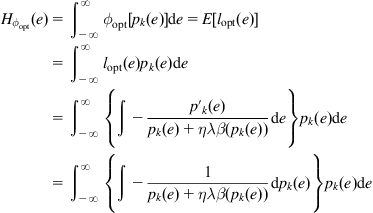 (4.196)
Hence
![]() (4.197)
(4.197)
Let ![]() , we obtain
, we obtain
![]() (4.198)
(4.198)
To achieve an explicit form of the function ![]() , we consider a special case in which the error is zero-mean Gaussian distributed:
, we consider a special case in which the error is zero-mean Gaussian distributed:
![]() (4.199)
(4.199)
Then we have
 (4.200)
It follows that
 (4.201)
Substituting Eq. (4.201) into Eq. (4.198) yields
![]() (4.202)
(4.202)
where ![]() ,
, ![]() , and
, and ![]() is a constant. Thus, we obtain the following optimal
is a constant. Thus, we obtain the following optimal ![]() -entropy:
-entropy:
![]() (4.203)
(4.203)
When ![]() , and
, and ![]() , we have
, we have
 (4.204)
That is, as ![]() the derived optimal entropy will approach the Shannon entropy. One may therefore conclude that, under slow adaptation condition (
the derived optimal entropy will approach the Shannon entropy. One may therefore conclude that, under slow adaptation condition (![]() is small enough), Shannon’s entropy is actually a suboptimal entropy criterion. Figure 4.22 shows the optimal
is small enough), Shannon’s entropy is actually a suboptimal entropy criterion. Figure 4.22 shows the optimal ![]() functions for different step-sizes
functions for different step-sizes ![]() (assume
(assume ![]() ).
).

Figure 4.22 Optimal ![]() functions for different step-sizes
functions for different step-sizes ![]() (adopted from Ref. [200]).
(adopted from Ref. [200]).
One can easily derive the IG algorithms under the optimal ![]() -entropy criterion. For example, substituting Eq. (4.202) into Eq. (4.79), we have the following SIG algorithm:
-entropy criterion. For example, substituting Eq. (4.202) into Eq. (4.79), we have the following SIG algorithm:
 (4.205)
It is worth noting that the above optimal ![]() entropy was derived as an example for a restricted situation, in which the constraints include FIR identification, white Gaussian input and noise, etc. For more general situations, such as nonlinear and non-Gaussian cases, the derived
entropy was derived as an example for a restricted situation, in which the constraints include FIR identification, white Gaussian input and noise, etc. For more general situations, such as nonlinear and non-Gaussian cases, the derived ![]() function would no longer be an optimal one.
function would no longer be an optimal one.
As pointed out in Ref. [28], the implementation of the optimal nonlinear error adaptation algorithm requires the exact knowledge of the noise’s or error’s PDFs. This is usually not the case in practice, since the characteristics of the noise or error may only be partially known or time-varying. In the implementation of the algorithm under the optimal ![]() -entropy criterion, however, the required PDFs are estimated by a nonparametric approach (say the KDE), and hence we don’t need such a priori information. It must be noted that in Eq. (4.205), the parameters
-entropy criterion, however, the required PDFs are estimated by a nonparametric approach (say the KDE), and hence we don’t need such a priori information. It must be noted that in Eq. (4.205), the parameters ![]() and
and ![]() are both related to the error variance
are both related to the error variance ![]() , which is always time-varying during the adaptation. In practice, we should estimate this variance and update the two parameters online.
, which is always time-varying during the adaptation. In practice, we should estimate this variance and update the two parameters online.
In the following, we present a simple numerical example to verify the theoretical conclusions and illustrate the improvements that may be achieved by optimizing the ![]() function. Consider the FIR system identification, where the transfer functions of the plant and the adaptive filter are [200]
function. Consider the FIR system identification, where the transfer functions of the plant and the adaptive filter are [200]
![]() (4.206)
(4.206)
The input signal and the noise are white Gaussian processes with powers 1.0 and 0.64, respectively. The initial weight vector of adaptive filter was obtained by perturbing each component of the optimal weight vector by a random variable that is uniformly distributed in the interval ![]() . In the simulation, the SIG algorithms under three different entropy criteria (optimal entropy, Shannon entropy, QIP) are compared. The Gaussian kernel is used and the kernel size is kept fixed at
. In the simulation, the SIG algorithms under three different entropy criteria (optimal entropy, Shannon entropy, QIP) are compared. The Gaussian kernel is used and the kernel size is kept fixed at ![]() during the adaptation.
during the adaptation.
First, the step-size of the SIG algorithm under the optimal entropy criterion was chosen to be ![]() . The step-sizes of the other two SIG algorithms are adjusted such that the three algorithms converge at the same initial rate. Figure 4.23 shows the average convergence curves over 300 simulation runs. Clearly, the optimal entropy criterion achieves the smallest final misadjustment (steady-state WEP). The step-sizes of the other two SIG algorithms can also be adjusted such that the three algorithms yield the same final misadjustment. The corresponding results are presented in Figure 4.24, which indicates that, beginning at the same initial WEP, the algorithm under optimal entropy criterion converges faster to the optimal solution than the other two algorithms. Therefore, a noticeable performance improvement can be achieved by optimizing the
. The step-sizes of the other two SIG algorithms are adjusted such that the three algorithms converge at the same initial rate. Figure 4.23 shows the average convergence curves over 300 simulation runs. Clearly, the optimal entropy criterion achieves the smallest final misadjustment (steady-state WEP). The step-sizes of the other two SIG algorithms can also be adjusted such that the three algorithms yield the same final misadjustment. The corresponding results are presented in Figure 4.24, which indicates that, beginning at the same initial WEP, the algorithm under optimal entropy criterion converges faster to the optimal solution than the other two algorithms. Therefore, a noticeable performance improvement can be achieved by optimizing the ![]() function.
function.

Figure 4.23 Convergence curves of three SIG algorithms with the same initial convergence rate (adopted from Ref. [200]).

Figure 4.24 Convergence curves of three SIG algorithms with the same final misadjustment (adopted from Ref. [200]).
Further, we consider the slow adaptation case in which the step-size for the optimal entropy criterion was chosen to be ![]() (smaller than 0.015). It has been proved that, if the step-size becomes smaller (tends to zero), the optimal entropy will approach the Shannon entropy. Thus, in this case, the adaptation behavior of the SIG algorithm under Shannon entropy criterion would be nearly equivalent to that of the optimal entropy criterion. This theoretical prediction is confirmed by Figure 4.25, which illustrates that the Shannon entropy criterion and the optimal entropy criterion may produce almost the same convergence performance. In this figure, the initial convergence rates of the three algorithms are set equal.
(smaller than 0.015). It has been proved that, if the step-size becomes smaller (tends to zero), the optimal entropy will approach the Shannon entropy. Thus, in this case, the adaptation behavior of the SIG algorithm under Shannon entropy criterion would be nearly equivalent to that of the optimal entropy criterion. This theoretical prediction is confirmed by Figure 4.25, which illustrates that the Shannon entropy criterion and the optimal entropy criterion may produce almost the same convergence performance. In this figure, the initial convergence rates of the three algorithms are set equal.

Figure 4.25 Convergence curves of three SIG algorithms in slow adaptation (adopted from Ref. [200]).
4.6 Survival Information Potential Criterion
Traditional entropy measures, such as Shannon and Renyi’s entropies of a continuous random variable, are defined based on the PDF. As argued by Rao et al. [157], this kind of entropy definition has several drawbacks: (i) the definition will be ill-suited for the case in which the PDF does not exist; (ii) the value can be negative; and (iii) the approximation using empirical distribution is impossible in general. In order to overcome these problems, Rao et al. proposed a new definition of entropy based on the cumulative distribution function (or equivalently, the survival function) of a random variable, which they called the cumulative residual entropy (CRE) [157]. Motivated by the definition of CRE, Zografos and Nadarajah proposed two new broad classes of entropy measures based on the survival function, that is, the survival exponential and generalized survival exponential entropies, which include the CRE as a special case [158].
In the following, a new IP, namely the survival information potential (SIP) [159] is defined in terms of the survival function instead of the density function. The basic idea of this definition is to replace the density function with the survival function in the expression of the traditional IP. The SIP is, in fact, the argument of the power function in the survival exponential entropy. In a sense, this parallels the relationship between the IP and the Renyi entropy. When used as an adaptation criterion, the SIP has some advantages over the IP: (i) it has consistent definition in the continuous and discrete domains; (ii) it is not shift-invariant (i.e., its value will vary with the location of distribution); (iii) it can be easily computed from sample data (without kernel computation and the choice of kernel width), and the estimation asymptotically converges to the true value; and (iv) it is a more robust measure since the distribution function is more regular than the density function (note that the density function is computed as the derivative of the distribution function).
4.6.1 Definition of SIP
Before proceeding, we review the definitions of the CRE and survival exponential entropy.
Let ![]() be a random vector in
be a random vector in ![]() . Denote
. Denote ![]() the absolute value transformed random vector of
the absolute value transformed random vector of ![]() , which is an
, which is an ![]() -dimensional random vector with components
-dimensional random vector with components ![]() . Then the CRE of
. Then the CRE of ![]() is defined by [157]
is defined by [157]
![]() (4.207)
(4.207)
where ![]() is the multivariate survival function of the random vector
is the multivariate survival function of the random vector ![]() , and
, and ![]() . Here the notation
. Here the notation ![]() means that
means that ![]() ,
, ![]() , and
, and ![]() denotes the indicator function.
denotes the indicator function.
Based on the same notations, the survival exponential entropy of order ![]() is defined as [158]
is defined as [158]
 (4.208)
From Eq. (4.208), we have
![]() (4.209)
(4.209)
It can be shown that the following limit holds [158]:
 (4.210)
The definition of the IP, along with the similarity between the survival exponential entropy and the Renyi entropy, motivates us to define the SIP.
Definition
For a random vector ![]() in
in ![]() , the SIP of order
, the SIP of order ![]() is defined by [159]
is defined by [159]
![]() (4.211)
(4.211)
The SIP (4.211) is just defined by replacing the density function with the survival function (of an absolute value transformation of ![]() ) in the original IP. This new definition seems more natural and reasonable, because the survival function (or equivalently, the distribution function) is more regular and general than the PDF. For the case
) in the original IP. This new definition seems more natural and reasonable, because the survival function (or equivalently, the distribution function) is more regular and general than the PDF. For the case ![]() , we call the SIP the quadratic survival information potential (QSIP).
, we call the SIP the quadratic survival information potential (QSIP).
The SIP ![]() can be interpreted as the
can be interpreted as the ![]() -power of the
-power of the ![]() -norm in the survival functional space. When
-norm in the survival functional space. When ![]() , the survival exponential entropy
, the survival exponential entropy ![]() is a monotonically increasing function of
is a monotonically increasing function of ![]() , and minimizing the SIP is equivalent to minimizing the survival exponential entropy; while when
, and minimizing the SIP is equivalent to minimizing the survival exponential entropy; while when ![]() , the survival exponential entropy
, the survival exponential entropy ![]() is a monotonically decreasing function of
is a monotonically decreasing function of ![]() , and in this case, minimizing the SIP is equivalent to maximizing the survival exponential entropy. We stress that when used as an approximation criterion in system identification, no matter what value of
, and in this case, minimizing the SIP is equivalent to maximizing the survival exponential entropy. We stress that when used as an approximation criterion in system identification, no matter what value of ![]() , the SIP should be minimized to achieve smaller errors. This is quite different from the IP criterion which should be maximized when
, the SIP should be minimized to achieve smaller errors. This is quite different from the IP criterion which should be maximized when ![]() [64]. The reason for this is that
[64]. The reason for this is that ![]() , the smaller SIP corresponds to more concentrated errors around the zero value. To demonstrate this fact, we give a simple example below.
, the smaller SIP corresponds to more concentrated errors around the zero value. To demonstrate this fact, we give a simple example below.
Assume that ![]() is zero-mean Gaussian distributed,
is zero-mean Gaussian distributed, ![]() . For different variance
. For different variance ![]() and
and ![]() values, we can calculate the SIP and IP, which are shown in Figure 4.26. It is clear that the SIP is a monotonically increasing function of
values, we can calculate the SIP and IP, which are shown in Figure 4.26. It is clear that the SIP is a monotonically increasing function of ![]() for all the
for all the ![]() values, while the IP is a monotonically increasing function only when
values, while the IP is a monotonically increasing function only when ![]() .
.
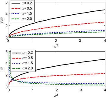
Figure 4.26 The SIP and IP for different ![]() and
and ![]() (adopted from Ref. [159]).
(adopted from Ref. [159]).
4.6.2 Properties of the SIP
To further understand the SIP, we present in the following some important properties.
Property 1:
![]() ,
, ![]() .
.
Property 2:
![]() , with equality if and only if
, with equality if and only if ![]() .
.
Proof:
It is obvious that ![]() . Now
. Now ![]() if and only if
if and only if ![]() . Therefore,
. Therefore, ![]() implies
implies ![]() for almost all
for almost all ![]() , or in other word, for almost all
, or in other word, for almost all ![]() ,
, ![]() , which implies
, which implies ![]() .
.
Remark:
The global minimum value of the SIP is zero, and it corresponds to the ![]() distribution located at zero. This is a desirable property that fails to hold for conventional MEE criteria whose global minimum corresponds to the
distribution located at zero. This is a desirable property that fails to hold for conventional MEE criteria whose global minimum corresponds to the ![]() distribution located at any position (shift-invariant). Hence when using SIP as an approximation criterion in system identification, we do not need to add a bias term at system output.
distribution located at any position (shift-invariant). Hence when using SIP as an approximation criterion in system identification, we do not need to add a bias term at system output.
The next five properties (Properties 3–7) are direct consequences of Ref. [158], and will, therefore, not be proved here (for detailed proofs, please refer to Theorems 1–5 in Ref. [158]).
Property 3:
If ![]() and
and ![]() (
(![]() ) for some
) for some ![]() , then
, then ![]() .
.
Property 4:
Let ![]() be an
be an ![]() -dimensional random vector, and let
-dimensional random vector, and let ![]() with
with ![]() ,
, ![]() ,
, ![]() . Then
. Then ![]() .
.
Property 5 (Weak convergence):
Let ![]() be a sequence of
be a sequence of ![]() -dimensional random vectors converging in law to a random vector
-dimensional random vectors converging in law to a random vector ![]() . If
. If ![]() are all bounded in
are all bounded in ![]() for some
for some![]() , then
, then ![]() .
.
Property 6:
If the components of an ![]() -dimensional random vector
-dimensional random vector ![]() are independent with each other, then
are independent with each other, then ![]() .
.
Property 7:
Let ![]() and
and ![]() be nonnegative and independent random variables (
be nonnegative and independent random variables (![]() ). Then
). Then ![]() .
.
Property 8:
Given two ![]() -dimensional continuous random vectors
-dimensional continuous random vectors ![]() and
and ![]() with PDFs
with PDFs ![]() and
and ![]() , if
, if ![]() is symmetric (rotation invariant for
is symmetric (rotation invariant for ![]() ) and unimodal around zero, and
) and unimodal around zero, and ![]() is independent of
is independent of ![]() , then
, then ![]() .
.
Proof:
Since ![]() and
and ![]() are independent,
are independent,
![]() (4.212)
(4.212)
It follows that ![]()
 (4.213)
where (a) follows from the condition that ![]() is symmetric (rotation invariance for
is symmetric (rotation invariance for ![]() ) and unimodal around zero. Thus we get
) and unimodal around zero. Thus we get ![]() .
.
Property 9:
For the case ![]() , the SIP of
, the SIP of ![]() equals the expectation of
equals the expectation of ![]() .
.
Proof:
 (4.214)
The above property can be generalized to the case where ![]() is a natural number, as stated in Property 10.
is a natural number, as stated in Property 10.
Property 10:
If ![]() , then
, then ![]() , where
, where ![]() ,
, ![]() are independent and identically distributed (i.i.d.) random vectors which are independent of but have the same distribution with
are independent and identically distributed (i.i.d.) random vectors which are independent of but have the same distribution with ![]() .
.
Proof:
As random vectors ![]() are i.i.d., independent of but have the same distribution with
are i.i.d., independent of but have the same distribution with ![]() , we can derive
, we can derive
 (4.215)
And hence
![]() (4.216)
(4.216)
The next property establishes a relationship between SIP and IP (which exists when ![]() has PDF). A similar relationship has been proved by Rao et al. for their CRE (see Proposition 4 in [157]).
has PDF). A similar relationship has been proved by Rao et al. for their CRE (see Proposition 4 in [157]).
Property 11:
Let ![]() be a nonnegative random variable with continuous distribution. Then there exists a function
be a nonnegative random variable with continuous distribution. Then there exists a function ![]() such that the
such that the ![]() -order IP of
-order IP of ![]() is related to
is related to ![]() via
via
![]() (4.217)
(4.217)
Proof:
Let ![]() be the distribution function with density
be the distribution function with density ![]() . If we choose
. If we choose ![]() , where
, where ![]() is defined as in the remarks preceding the Proposition 4 in [157], then
is defined as in the remarks preceding the Proposition 4 in [157], then ![]() has the distribution
has the distribution ![]() . Therefore, we have
. Therefore, we have
![]() (4.218)
(4.218)
Property 12:
Let ![]() and
and ![]() be two continuous random vectors. Assuming for every value
be two continuous random vectors. Assuming for every value ![]() , the conditional density
, the conditional density ![]() is symmetric (rotation invariant for
is symmetric (rotation invariant for ![]() ) and unimodal in
) and unimodal in ![]() around
around ![]() , then
, then ![]() , where
, where ![]() is any mapping
is any mapping ![]() for which
for which ![]() exists.
exists.
Proof:
Denote ![]() and
and ![]() , respectively, the densities of
, respectively, the densities of ![]() and
and ![]() , i.e.,
, i.e.,
![]() (4.219)
(4.219)
Then for any ![]() , we have
, we have
 (4.220)
where (b) comes from the condition that for every ![]() ,
, ![]() is symmetric (rotation invariant for
is symmetric (rotation invariant for ![]() ) and unimodal in
) and unimodal in ![]() around
around ![]() . Therefore
. Therefore
![]() (4.221)
(4.221)
Remark:
The above property suggests that under certain conditions, the conditional mean ![]() , which minimizes the MSE, also minimizes the error’s SIP.
, which minimizes the MSE, also minimizes the error’s SIP.
4.6.3 Empirical SIP
Next, we discuss the empirical SIP of ![]() . Since
. Since ![]() (see Property 1), we assume without loss of generality that
(see Property 1), we assume without loss of generality that ![]() . Let
. Let ![]() be
be ![]() i.i.d. samples of
i.i.d. samples of ![]() with survival function
with survival function ![]() . The empirical survival function of
. The empirical survival function of ![]() can be estimated by putting 1/N at each of the sample points, i.e.,
can be estimated by putting 1/N at each of the sample points, i.e.,
![]() (4.222)
(4.222)
Consequently, the empirical SIP can be calculated as
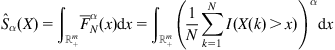 (4.223)
According to Glivento–Cantelli theorem [202],
![]() (4.224)
(4.224)
Combining Eq. (4.224) and Property 5 yields the following proposition.
Proposition:
For any random vector ![]() in
in ![]() , if
, if ![]() is bounded in
is bounded in ![]() for some
for some ![]() , then the empirical SIP (4.223) will converge to the true SIP of
, then the empirical SIP (4.223) will converge to the true SIP of ![]() , i.e.,
, i.e., ![]() .
.
In the sequel, we will derive more explicit expressions for the empirical SIP (4.223). Let ![]() be a realization of
be a realization of ![]() .
.
4.6.3.1 Scalar Data Case
First, we consider the scalar data case, i.e., ![]() . We assume, without loss of generality, that
. We assume, without loss of generality, that ![]() . Then we derive
. Then we derive
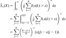 (4.225)
where we assume ![]() . One can rewrite Eq. (4.225) into a more simple form:
. One can rewrite Eq. (4.225) into a more simple form:
 (4.226)
where
![]() (4.227)
(4.227)
From Eq. (4.226), the empirical SIP for scalar data can be expressed as a weighted sum of the ordered sample data ![]() , where the weights
, where the weights ![]() depend on the sample size
depend on the sample size ![]() and the
and the ![]() value, satisfying
value, satisfying ![]() ,
, ![]() . For the case
. For the case ![]() , the weights for different
, the weights for different ![]() values are shown in Figure 4.27. One can observe: (i) when
values are shown in Figure 4.27. One can observe: (i) when ![]() , all the weights are equal (
, all the weights are equal (![]() ), and in this case the empirical SIP is identical to the sample mean of
), and in this case the empirical SIP is identical to the sample mean of ![]() and (ii) when
and (ii) when ![]() , the weights are not equal. Specifically, when
, the weights are not equal. Specifically, when ![]() (
(![]() ), the weight
), the weight ![]() is a monotonically increasing (decreasing) function of the order index
is a monotonically increasing (decreasing) function of the order index ![]() , that is, the larger weights are assigned to the larger (smaller) sample data.
, that is, the larger weights are assigned to the larger (smaller) sample data.

Figure 4.27 The weights for different ![]() values (adopted from Ref. [159]).
values (adopted from Ref. [159]).
4.6.3.2 Multidimensional Data Case
Computing the empirical SIP for multidimensional data (![]() ) is, in general, not an easy task. If
) is, in general, not an easy task. If ![]() is a natural number, however, we can still obtain a simple explicit expression. In this case, one can derive
is a natural number, however, we can still obtain a simple explicit expression. In this case, one can derive
 (4.228)
The empirical SIP in Eq. (4.228) can also be derived using Property 10. By Property 10, we have ![]() , where
, where ![]() are i.i.d. random vectors which are independent of but have the same distribution with
are i.i.d. random vectors which are independent of but have the same distribution with ![]() . It is now evident that the empirical SIP of Eq. (4.228) is actually the sample mean estimate of
. It is now evident that the empirical SIP of Eq. (4.228) is actually the sample mean estimate of ![]() .
.
4.6.4 Application to System Identification
Similar to the IP, the SIP can also be used as an optimality criterion in adaptive system training. Under the SIP criterion, the unknown system parameter vector (or weight vector) ![]() can be estimated as
can be estimated as
![]() (4.229)
(4.229)
where ![]() is the survival function of the absolute value transformed error
is the survival function of the absolute value transformed error ![]() . In practical application, the error distribution is usually unknown; we have to use, instead of the theoretical SIP, the empirical SIP as the cost function. Given a sequence of error samples
. In practical application, the error distribution is usually unknown; we have to use, instead of the theoretical SIP, the empirical SIP as the cost function. Given a sequence of error samples ![]() , assuming, without loss of generality, that
, assuming, without loss of generality, that ![]() , the empirical SIP will be (assume scalar error)
, the empirical SIP will be (assume scalar error)
![]() (4.230)
(4.230)
where ![]() is calculated by Eq. (4.227). The empirical cost (4.230) is a weighted sum of the ordered absolute errors. One drawback of Eq. (4.230) is that it is not smooth at
is calculated by Eq. (4.227). The empirical cost (4.230) is a weighted sum of the ordered absolute errors. One drawback of Eq. (4.230) is that it is not smooth at ![]() . To address this problem, one can use the empirical SIP of the square errors
. To address this problem, one can use the empirical SIP of the square errors ![]() as an alternative adaptation cost, given by
as an alternative adaptation cost, given by
![]() (4.231)
(4.231)
The above cost is the weighted sum of the ordered square errors, which includes the popular MSE cost as a special case (when ![]() ). A more general cost can be defined as the empirical SIP of any mapped errors
). A more general cost can be defined as the empirical SIP of any mapped errors ![]() , i.e.,
, i.e.,
![]() (4.232)
(4.232)
where function ![]() usually satisfies
usually satisfies
 (4.233)
Based on the general cost (4.232), the weight update equation for system identification is
![]() (4.234)
(4.234)
The weight update can be performed online (i.e., over a short sliding window), as described in Table 4.5.

In the following, we present two simulation examples to demonstrate the performance of the SIP minimization criterion. In the simulations below, the empirical cost (4.231) is adopted (![]() ).
).
4.6.4.1 FIR System Identification
First, we consider the simple FIR system identification. Let the unknown system be a FIR filter given by [159]
![]() (4.235)
(4.235)
The adaptive system is another FIR filter with the same order. The input ![]() is a white Gaussian process with unit variance. Assume that the output of unknown system is disturbed by an additive noise. Three different distributions are utilized to generate the noise data:
is a white Gaussian process with unit variance. Assume that the output of unknown system is disturbed by an additive noise. Three different distributions are utilized to generate the noise data:
 (4.236)
where ![]() denotes the characteristic function of the
denotes the characteristic function of the ![]() distribution. The above three distributions have, respectively, heavy, medium, and light tails. The noise signals are shown in Figure 4.28.
distribution. The above three distributions have, respectively, heavy, medium, and light tails. The noise signals are shown in Figure 4.28.

In the simulation, the sliding data length is set at 10. The step-sizes of each algorithm are chosen such that the initial convergence rates are visually identical. Figure 4.29 shows the average convergence curves over 100 Monte Carlo runs for different ![]() . Notice that when
. Notice that when ![]() , the algorithm is actually the LMS algorithm (strictly speaking, the block LMS algorithm). The WEPs at final iteration are summarized in Table 4.6. From simulation results, one can observe:
, the algorithm is actually the LMS algorithm (strictly speaking, the block LMS algorithm). The WEPs at final iteration are summarized in Table 4.6. From simulation results, one can observe:
i. For the case of ![]() noise, the algorithms with larger
noise, the algorithms with larger ![]() values (say
values (say ![]() ) converge to smaller WEP, and can even outperform the LAD algorithm (for comparison purpose, we also plot in Figure 4.29(A) the convergence curve of LAD). It is well known that the LAD algorithm performs well in
) converge to smaller WEP, and can even outperform the LAD algorithm (for comparison purpose, we also plot in Figure 4.29(A) the convergence curve of LAD). It is well known that the LAD algorithm performs well in ![]() -stable noises [31].
-stable noises [31].
ii. For the case of Gaussian noise, the algorithm with ![]() (the LMS algorithm) performs better, which is to be expected, since MSE criterion is optimal for linear Gaussian systems.
(the LMS algorithm) performs better, which is to be expected, since MSE criterion is optimal for linear Gaussian systems.
iii. For the case of binary noise, the algorithms with smaller ![]() values (say
values (say ![]() ) obtain better performance.
) obtain better performance.

Figure 4.29 Convergence curves averaged over 100 Monte Carlo runs: (A) ![]() , (B) Gaussian, and (C) Binary.
, (B) Gaussian, and (C) Binary.

The basic reasons for these findings are as follows. As shown in Figure 4.27, the larger the ![]() value, the smaller the weights assigned to the larger errors. For the case of heavy-tail noises (e.g.,
value, the smaller the weights assigned to the larger errors. For the case of heavy-tail noises (e.g., ![]() noise), the larger errors are usually caused by the impulsive noise. In this case, the larger
noise), the larger errors are usually caused by the impulsive noise. In this case, the larger ![]() value will reduce the influence of the outliers and improve the performance. On the other hand, for the case of light-tail noises (e.g., binary noise), the larger errors are mainly caused by the system mismatch, thus the smaller
value will reduce the influence of the outliers and improve the performance. On the other hand, for the case of light-tail noises (e.g., binary noise), the larger errors are mainly caused by the system mismatch, thus the smaller ![]() value will decrease the larger mismatch more rapidly (as the larger weights are assigned to the larger errors).
value will decrease the larger mismatch more rapidly (as the larger weights are assigned to the larger errors).
4.6.4.2 TDNN Training
The second simulation example is on the TDNNs training (in batch mode) with SIP minimization criterion for one-step prediction of the Mackey–Glass (MG) chaotic time series [203] with delay parameter ![]() and sampling period 6 s. The TDNN is built from MLPs that consist of six processing elements (PEs) in a hidden layer with biases and tanh nonlinearities and a single linear output PE with an output bias. The goal is to predict the value of the current sample
and sampling period 6 s. The TDNN is built from MLPs that consist of six processing elements (PEs) in a hidden layer with biases and tanh nonlinearities and a single linear output PE with an output bias. The goal is to predict the value of the current sample ![]() using the previous seven points
using the previous seven points ![]() (the size of the input delay line is consistent with Taken’s embedding theorem [204]). In essence, the problem is to identify the underlying mapping between the input vector
(the size of the input delay line is consistent with Taken’s embedding theorem [204]). In essence, the problem is to identify the underlying mapping between the input vector ![]() and the desired output
and the desired output ![]() . For comparison purpose, we also present simulation results of TDNN training with
. For comparison purpose, we also present simulation results of TDNN training with ![]() -order (
-order (![]() ) IP maximization criterion. Since IP is shift-invariant, after training the bias value of the output PE was adjusted so as to yield zero-mean error over the training set. The Gaussian kernel was used to evaluate the empirical IP and the kernel size was experimentally set at 0.8. A segment of 200 samples is used as the training data. To avoid local-optimal solutions, each TDNN is trained starting from 500 predetermined initial weights generated by zero-mean Gaussian distribution with variance 0.01. The best solution (the one with the lowest SIP or the highest IP after training) among the 500 candidates is selected to test the accuracy performance. In each simulation, the training algorithms utilized BP with variable step-sizes [205], and 1000 iterations were run to ensure the convergence. The trained networks are tested on an independently generated test sequence of 4000 samples, and the testing errors are listed in Table 4.7. One can see the TDNN trained using SIP with
) IP maximization criterion. Since IP is shift-invariant, after training the bias value of the output PE was adjusted so as to yield zero-mean error over the training set. The Gaussian kernel was used to evaluate the empirical IP and the kernel size was experimentally set at 0.8. A segment of 200 samples is used as the training data. To avoid local-optimal solutions, each TDNN is trained starting from 500 predetermined initial weights generated by zero-mean Gaussian distribution with variance 0.01. The best solution (the one with the lowest SIP or the highest IP after training) among the 500 candidates is selected to test the accuracy performance. In each simulation, the training algorithms utilized BP with variable step-sizes [205], and 1000 iterations were run to ensure the convergence. The trained networks are tested on an independently generated test sequence of 4000 samples, and the testing errors are listed in Table 4.7. One can see the TDNN trained using SIP with ![]() achieves the smallest testing error. Thus, if properly choosing the order
achieves the smallest testing error. Thus, if properly choosing the order ![]() , the SIP criterion is capable of outperforming the IP criterion. Figure 4.30 shows the computation time per iteration versus the number of training data. Clearly, the SIP-based training is computationally much more efficient than the IP-based training, especially for large data sets. The training time for both methods is measured on a personal computer equipped with a 2.2 GHz Processor and 3 GB memory.
, the SIP criterion is capable of outperforming the IP criterion. Figure 4.30 shows the computation time per iteration versus the number of training data. Clearly, the SIP-based training is computationally much more efficient than the IP-based training, especially for large data sets. The training time for both methods is measured on a personal computer equipped with a 2.2 GHz Processor and 3 GB memory.


4.7 Δ-Entropy Criterion
System identification usually handles continuous-valued random processes rather than discrete-valued processes. In many practical situations, however, the input and/or output of the unknown system may be discrete-valued for a variety of reasons:
a. For many systems, especially in the field of digital communication, the input signals take values only in finite alphabetical sets.
b. Coarsely quantized signals are commonly used when the data are obtained from an A/D converter or from a communication channel. Typical contexts involving quantized data include digital control systems (DCSs), networked control systems (NCSs), wireless sensor networks (WSNs), etc.
c. Binary-valued sensors occur frequently in practical systems. Some typical examples of binary-valued sensors can be found in Ref. [206].
d. Discrete-valued time series are common in practice. In recent years, the count or integer-valued data time series have gained increasing attentions [207–210].
e. Sometimes, due to computational consideration, even if the observed signals are continuous-valued, one may classify the data into groups and obtain the discrete-valued data [130, Chap. 5].
In these situations, one may apply the differential entropy (or IP) to implement the MEE criterion, in spite of the fact that the random variables are indeed discrete. When the discretization is coarse (i.e., few levels) the use of differential entropy may carry a penalty in performance that is normally not quantified. Alternatively, the MEE implemented with discrete entropy will become ill-suited since the minimization fails to constrain the dispersion of the error value which should be pursued because the error dynamic range decreases over iterations.
In the following, we augment the MEE criterion choices by providing a new entropy definition for discrete random variables, called the ![]() -entropy, which comprises two terms: one is the discrete entropy and the other is the logarithm of the average interval between two successive discrete values. This new entropy retains important properties of the differential entropy and reduces to the traditional discrete entropy for a special case. More importantly, the proposed entropy definition can still be used to measure the value dispersion of a discrete random variable, and hence can be used as an MEE optimality criterion in system identification with discrete-valued data.
-entropy, which comprises two terms: one is the discrete entropy and the other is the logarithm of the average interval between two successive discrete values. This new entropy retains important properties of the differential entropy and reduces to the traditional discrete entropy for a special case. More importantly, the proposed entropy definition can still be used to measure the value dispersion of a discrete random variable, and hence can be used as an MEE optimality criterion in system identification with discrete-valued data.
4.7.1 Definition of Δ-Entropy
Before giving the definition of ![]() -entropy, let’s review a fundamental relationship between the differential entropy and discrete entropy (for details, see also Ref. [43]).
-entropy, let’s review a fundamental relationship between the differential entropy and discrete entropy (for details, see also Ref. [43]).
Consider a continuous scalar random variable ![]() with PDF
with PDF ![]() . One can produce a quantized random variable
. One can produce a quantized random variable ![]() (see Figure 4.31), given by
(see Figure 4.31), given by
![]() (4.237)
(4.237)
where ![]() is one of countable values, satisfying
is one of countable values, satisfying
![]() (4.238)
(4.238)

The probability that ![]() is
is
![]() (4.239)
(4.239)
And hence, the discrete entropy ![]() is calculated as
is calculated as
![]() (4.240)
(4.240)
If the density function ![]() is Riemann integrable, the following limit holds
is Riemann integrable, the following limit holds
![]() (4.241)
(4.241)
Here, to make a distinction between the discrete entropy and differential entropy, we use ![]() instead of
instead of ![]() to denote the differential entropy of
to denote the differential entropy of ![]() . Thus, if the quantization interval
. Thus, if the quantization interval ![]() is small enough, we have
is small enough, we have
![]() (4.242)
(4.242)
So, the differential entropy of a continuous random variable ![]() is approximately equal to the discrete entropy of the quantized variable
is approximately equal to the discrete entropy of the quantized variable ![]() plus the logarithm of the quantization interval
plus the logarithm of the quantization interval ![]() . The above relationship explains why differential entropy is sensitive to value dispersion. That is, compared with the discrete entropy, the differential entropy “contains” the term
. The above relationship explains why differential entropy is sensitive to value dispersion. That is, compared with the discrete entropy, the differential entropy “contains” the term ![]() , which measures the average interval between two successive quantized values since
, which measures the average interval between two successive quantized values since
![]() (4.243)
(4.243)
This important relationship also inspired us to seek a new entropy definition for discrete random variables that will measure uncertainty as well as value dispersion and is defined as follows.
Definition: Given a discrete random variable ![]() with values
with values ![]() , and the corresponding distribution
, and the corresponding distribution ![]() , the
, the ![]() -entropy, denoted by
-entropy, denoted by ![]() or
or ![]() , is defined as [211]
, is defined as [211]
![]() (4.244)
(4.244)
where ![]() (or
(or ![]() ) stands for the average interval (distance) between two successive values.
) stands for the average interval (distance) between two successive values.
The ![]() -entropy contains two terms: the first term is identical to the traditional discrete entropy and the second term equals the logarithm of the average interval between two successive values. This new entropy can be used as an optimality criterion in estimation or identification problems, because minimizing error’s
-entropy contains two terms: the first term is identical to the traditional discrete entropy and the second term equals the logarithm of the average interval between two successive values. This new entropy can be used as an optimality criterion in estimation or identification problems, because minimizing error’s ![]() -entropy decreases the average interval and automatically force the error values to concentrate.
-entropy decreases the average interval and automatically force the error values to concentrate.
Next, we discuss how to calculate the average interval ![]() . Assume without loss of generality that the discrete values satisfy
. Assume without loss of generality that the discrete values satisfy ![]() . Naturally, one immediately thinks of the arithmetic and geometric means, i.e.,
. Naturally, one immediately thinks of the arithmetic and geometric means, i.e.,
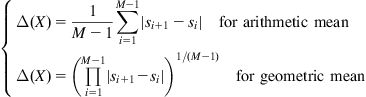 (4.245)
Both arithmetic and geometric means take no account of the distribution. A more reasonable approach is to calculate the average interval using a probability-weighted method. For example, one can use the following formula:
![]() (4.246)
(4.246)
However, if ![]() , the sum of weights will be <1, because
, the sum of weights will be <1, because
![]() (4.247)
(4.247)
To address this issue, we give another formula:
![]() (4.248)
(4.248)
The second term of (4.248) equals the arithmetic mean multiplied by ![]() , which normalizes the weight sum to one. Substituting (4.248) into (4.244), we obtain
, which normalizes the weight sum to one. Substituting (4.248) into (4.244), we obtain
 (4.249)
The ![]() -entropy can be immediately extended to the infinite value-set case, i.e.,
-entropy can be immediately extended to the infinite value-set case, i.e.,
 (4.250)
In the following, we use Eq. (4.249) or (4.250) as the ![]() -entropy expression.
-entropy expression.
4.7.2 Some Properties of the Δ-Entropy
The ![]() -entropy maintains a close connection to the differential entropy. It is clear that the
-entropy maintains a close connection to the differential entropy. It is clear that the ![]() -entropy and the differential entropy have the following relationship in the limit:
-entropy and the differential entropy have the following relationship in the limit:
Theorem 1
For any continuous random variable ![]() with Riemann integrable PDF
with Riemann integrable PDF ![]() , we have
, we have ![]() , where quantized variable
, where quantized variable ![]() is given by Eq. (4.237).
is given by Eq. (4.237).
Proof:
Combining Eqs. (4.239) and (4.250), we have

As ![]() is Riemann integrable, it follows that
is Riemann integrable, it follows that
![]()
This completes the proof.
Remark:
The differential entropy of ![]() is the limit of the
is the limit of the ![]() -entropy of
-entropy of ![]() as
as ![]() . Thus, to some extent one can regard the
. Thus, to some extent one can regard the ![]() -entropy as a “quantized version” of the differential entropy.
-entropy as a “quantized version” of the differential entropy.
Theorem 2
![]() .
.
Remark:
By Theorem 2, if the minimum interval between two successive values is larger than 1, we have ![]() , whereas if the maximum interval between two successive values is smaller than 1, we have
, whereas if the maximum interval between two successive values is smaller than 1, we have ![]() .
.
Theorem 3
If ![]() is a discrete random variable with equally spaced values, and the interval
is a discrete random variable with equally spaced values, and the interval ![]() , then
, then ![]() .
.
Proof:
For equally spaced intervals, the difference between the![]() -entropy and the discrete entropy equals
-entropy and the discrete entropy equals ![]() . Hence, the statement follows directly.
. Hence, the statement follows directly.
Remark:
The classification problem is, in general, a typical example of the error variable distributed on equally spaced values ![]() . Thus in classification, the error’s discrete entropy is equivalent to the
. Thus in classification, the error’s discrete entropy is equivalent to the ![]() -entropy. This fact also gives an interpretation for why the discrete entropy can be used in the test and classification problems [212,213].
-entropy. This fact also gives an interpretation for why the discrete entropy can be used in the test and classification problems [212,213].
In information theory, it has been proved that the discrete entropy satisfies (see Ref. [43], p. 489)
 (4.251)
Combining Eq. (4.251) and Theorem 2, we obtain a bound on ![]() -entropy:
-entropy:
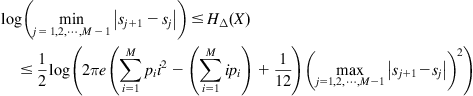 (4.252)
A lower bound of the ![]() -entropy can also be expressed in terms of the variance
-entropy can also be expressed in terms of the variance ![]() , as given in the following theorem:
, as given in the following theorem:
Theorem 4
If ![]() , then
, then ![]() .
.
Proof:
It is easy to derive

It follows that ![]() , and hence
, and hence
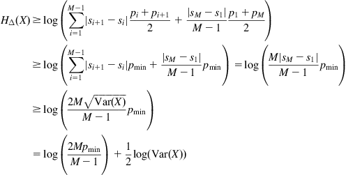
The lower bound of Theorem 4 suggests that, under certain condition minimizing the ![]() -entropy constrains the variance. This is a key difference between the
-entropy constrains the variance. This is a key difference between the ![]() -entropy and conventional discrete entropy.
-entropy and conventional discrete entropy.
Theorem 5
For any discrete random variable ![]() ,
, ![]() ,
, ![]() .
.
Proof:
Since ![]() and
and ![]() , we have
, we have![]() .
.
Theorem 6
![]() ,
, ![]() .
.
Proof:
Since ![]() and
and ![]() , we have
, we have ![]() .
.
Theorems 5 and 6 indicate that the ![]() -entropy has the same shifting and scaling properties as the differential entropy.
-entropy has the same shifting and scaling properties as the differential entropy.
Theorem 7
The ![]() -entropy is a concave function of
-entropy is a concave function of ![]() .
.
Proof:
![]() , and
, and ![]() , we have
, we have
![]() (4.253)
(4.253)
By the concavity of the logarithm function,
![]() (4.254)
(4.254)
It is well known that the discrete entropy ![]() is a concave function of the distribution
is a concave function of the distribution ![]() , i.e.,
, i.e.,
![]() (4.255)
(4.255)
Combining Eqs. (4.254) and (4.255) yields
![]() (4.256)
(4.256)
which implies ![]() -entropy is a concave function of
-entropy is a concave function of ![]() .
.
The concavity of the ![]() -entropy is a desirable property for the entropy optimization problem. This property ensures that when a stationary value of the
-entropy is a desirable property for the entropy optimization problem. This property ensures that when a stationary value of the ![]() -entropy subject to linear constraints is found, it gives the global maximum value [149].
-entropy subject to linear constraints is found, it gives the global maximum value [149].
Next, we solve the maximum ![]() -entropy distribution. Consider the following constrained optimization problem:
-entropy distribution. Consider the following constrained optimization problem:
 (4.257)
where ![]() is the expected value of the function
is the expected value of the function ![]() . The Lagrangian is given by
. The Lagrangian is given by
 (4.258)
where ![]() are the
are the ![]() Lagrange multipliers corresponding to the
Lagrange multipliers corresponding to the ![]() constraints. Here
constraints. Here ![]() is used as the first Lagrange multiplier instead of
is used as the first Lagrange multiplier instead of ![]() as a matter of convenience. Let
as a matter of convenience. Let ![]() , we have
, we have
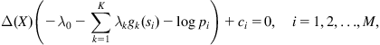 (4.259)
where
 (4.260)
Solving Eq. (4.259), we obtain the following theorem:
Theorem 8
The distribution ![]() that maximizes the
that maximizes the ![]() -entropy subject to the constraints of Eq. (4.257) is given by
-entropy subject to the constraints of Eq. (4.257) is given by
 (4.261)
where ![]() are determined by substituting for
are determined by substituting for ![]() from Eq. (4.261) into the constraints of Eq. (4.257).
from Eq. (4.261) into the constraints of Eq. (4.257).
For the case in which the discrete values are equally spaced, we have ![]() , and Eq. (4.261) becomes
, and Eq. (4.261) becomes
 (4.262)
In this case, the maximum ![]() -entropy distribution is identical to the maximum discrete entropy distribution [149].
-entropy distribution is identical to the maximum discrete entropy distribution [149].
4.7.3 Estimation of Δ-Entropy
In practical situations, the discrete values ![]() and probabilities
and probabilities ![]() are usually unknown, and we must estimate them from sample data
are usually unknown, and we must estimate them from sample data ![]() . An immediate approach is to group the sample data into different values
. An immediate approach is to group the sample data into different values ![]() and calculate the corresponding relative frequencies:
and calculate the corresponding relative frequencies:
![]() (4.263)
(4.263)
where ![]() denotes the number of these outcomes belonging to the value
denotes the number of these outcomes belonging to the value ![]() with
with ![]() .
.
Based on the estimated values ![]() and probabilities
and probabilities ![]() , a simple plug-in estimate of
, a simple plug-in estimate of ![]() -entropy can be obtained as
-entropy can be obtained as
 (4.264)
As the sample size increases, the estimated value set ![]() will approach the true value set
will approach the true value set ![]() with probability one, i.e.,
with probability one, i.e., ![]() , as
, as ![]() . In fact, assuming
. In fact, assuming ![]() is an i.i.d. sample from the distribution
is an i.i.d. sample from the distribution ![]() , and
, and ![]() ,
, ![]() , we have
, we have
 (4.265)
We investigate in the following the asymptotic behavior of the ![]() -entropy in random sampling. We assume for tractability that the value set
-entropy in random sampling. We assume for tractability that the value set ![]() is known (or has been exactly estimated). Following a similar derivation of the asymptotic distribution for the
is known (or has been exactly estimated). Following a similar derivation of the asymptotic distribution for the ![]() -entropy (see Ref. [130], Chap. 2), we denote the parameter vector
-entropy (see Ref. [130], Chap. 2), we denote the parameter vector ![]() , and rewrite Eq. (4.264) as
, and rewrite Eq. (4.264) as
 (4.266)
The first-order Taylor expansion of ![]() around
around ![]() gives
gives
![]() (4.267)
(4.267)
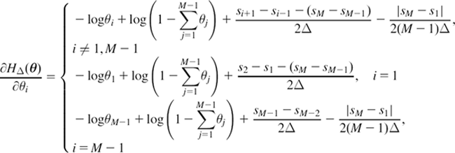 (4.268)
where
 (4.269)
According to Ref. [130, Chap. 2], we have
![]() (4.270)
(4.270)
where the inverse of the Fisher information matrix of ![]() is given by
is given by ![]() . Then
. Then ![]() is bounded in probability, and
is bounded in probability, and
![]() (4.271)
(4.271)
And hence, random variables ![]() and
and ![]() have the same asymptotic distribution, and we have the following theorem.
have the same asymptotic distribution, and we have the following theorem.
Theorem 9
The estimate ![]() , obtained by replacing the
, obtained by replacing the ![]() by their relative frequencies
by their relative frequencies ![]() , in a random sample of size
, in a random sample of size ![]() , satisfies
, satisfies
![]() (4.272)
(4.272)
provided ![]() , where
, where ![]() ,
, ![]() , and
, and
![]() (4.273)
(4.273)
where ![]() is calculated as (4.268).
is calculated as (4.268).
The afore-discussed plug-in estimator of the ![]() -entropy has close relationships with certain estimators of the differential entropy.
-entropy has close relationships with certain estimators of the differential entropy.
4.7.3.1 Relation to KDE-based Differential Entropy Estimator
Suppose ![]() are samples from a discrete random variable
are samples from a discrete random variable ![]() . We rewrite the plug-in estimate (4.264) as
. We rewrite the plug-in estimate (4.264) as
![]() (4.274)
(4.274)
where ![]() . Denote
. Denote ![]() , and let
, and let ![]() , we construct another set of samples:
, we construct another set of samples:
![]() (4.275)
(4.275)
which are samples from the discrete random variable ![]() , and satisfy
, and satisfy
![]() (4.276)
(4.276)
Now we consider ![]() as samples from a “continuous” random variable
as samples from a “continuous” random variable ![]() . The PDF of
. The PDF of ![]() can be estimated by the KDE approach:
can be estimated by the KDE approach:
![]() (4.277)
(4.277)
The kernel function satisfies ![]() and
and ![]() . If the kernel function is selected as the following uniform kernel:
. If the kernel function is selected as the following uniform kernel:
 (4.278)
then Eq. (4.277) becomes
 (4.279)
where ![]() follows from
follows from ![]() , and
, and ![]() ,
, ![]() . The differential entropy of
. The differential entropy of ![]() can then be estimated as
can then be estimated as
 (4.280)
As a result, the plug-in estimate of the ![]() -entropy is identical to a uniform kernel-based estimate of the differential entropy from the scaled samples (4.275).
-entropy is identical to a uniform kernel-based estimate of the differential entropy from the scaled samples (4.275).
4.7.3.2 Relation to Sample-Spacing Based Differential Entropy Estimator
The plug-in estimate of the ![]() -entropy also has a close connection with the sample-spacing based estimate of the differential entropy. Suppose the sample data are different from each other, and have been rearranged in an increasing order:
-entropy also has a close connection with the sample-spacing based estimate of the differential entropy. Suppose the sample data are different from each other, and have been rearranged in an increasing order: ![]() , the
, the ![]() -spacing estimate is given by [214]
-spacing estimate is given by [214]
![]() (4.281)
(4.281)
where ![]() and
and ![]() . If
. If ![]() , we obtain the one-spacing estimate:
, we obtain the one-spacing estimate:
![]() (4.282)
(4.282)
On the other hand, based on the samples one can estimate the value set and corresponding probabilities:
![]() (4.283)
(4.283)
Then the plug-in estimate of the ![]() -entropy will be
-entropy will be
 (4.284)
It follows that
 (4.285)
where (b) comes from the concavity of the logarithm function. If ![]() is bounded, we have
is bounded, we have
![]() (4.286)
(4.286)
In this case, the plug-in estimate of ![]() -entropy provides an asymptotic upper bound on the one-spacing entropy estimate.
-entropy provides an asymptotic upper bound on the one-spacing entropy estimate.
4.7.4 Application to System Identification
The ![]() -entropy can be used as an optimality criterion in system identification, especially when error signal is distributed on a countable value set (which is usually unknown and varying with time) 15. A typical example is the system identification with quantized input/output (I/O) data, as shown in Figure 4.32, where
-entropy can be used as an optimality criterion in system identification, especially when error signal is distributed on a countable value set (which is usually unknown and varying with time) 15. A typical example is the system identification with quantized input/output (I/O) data, as shown in Figure 4.32, where ![]() and
and ![]() represent the quantized I/O observations, obtained via I/O quantizers
represent the quantized I/O observations, obtained via I/O quantizers ![]() and
and ![]() . With uniform quantization,
. With uniform quantization, ![]() and
and ![]() can be expressed as
can be expressed as
![]() (4.287)
(4.287)
where ![]() and
and ![]() denote the quantization box-sizes,
denote the quantization box-sizes, ![]() gives the largest integer that is less than or equal to
gives the largest integer that is less than or equal to ![]() .
.

In practice, ![]() -entropy cannot be, in general, analytically computed, since the error’s values and corresponding probabilities are unknown. In this case, we need to estimate the
-entropy cannot be, in general, analytically computed, since the error’s values and corresponding probabilities are unknown. In this case, we need to estimate the ![]() -entropy by the plug-in method as discussed previously. Traditional gradient-based methods, however, cannot be used to solve the
-entropy by the plug-in method as discussed previously. Traditional gradient-based methods, however, cannot be used to solve the ![]() -entropy minimization problem, since the objective function is usually not differentiable. Thus, we have to resort to other methods, such as the estimation of distribution algorithms (EDAs) [215], a new class of evolutionary algorithms (EAs), although they are usually more computationally complex. The EDAs use the probability model built from the objective function to generate the promising search points instead of crossover and mutation as done in traditional GAs. Some theoretical results related to the convergence and time complexity of EDAs can be found in Ref. [215]. Table 4.8 presents the EDA-based identification algorithm with
-entropy minimization problem, since the objective function is usually not differentiable. Thus, we have to resort to other methods, such as the estimation of distribution algorithms (EDAs) [215], a new class of evolutionary algorithms (EAs), although they are usually more computationally complex. The EDAs use the probability model built from the objective function to generate the promising search points instead of crossover and mutation as done in traditional GAs. Some theoretical results related to the convergence and time complexity of EDAs can be found in Ref. [215]. Table 4.8 presents the EDA-based identification algorithm with ![]() -entropy criterion.
-entropy criterion.

Usually, we use a Gaussian model with diagonal covariance matrix (GM/DCM) [215] to estimate the density function ![]() of the
of the ![]() th generation. With GM/DCM model, we have
th generation. With GM/DCM model, we have
![]() (4.288)
(4.288)
where the means ![]() and the deviations
and the deviations ![]() can be estimated as
can be estimated as
 (4.289)
In the following, two simple examples are presented to demonstrate the performance of the above algorithm. In all of the simulations below, we set ![]() and
and ![]() .
.
First, we consider the system identification based on quantized I/O data, where the unknown system and the parametric model are both two-tap FIR filters, i.e.,
![]() (4.290)
(4.290)
The true weight vector of the unknown system is ![]() , and the initial weight vector of the model is
, and the initial weight vector of the model is ![]() . The input signal and the additive noise are both white Gaussian processes with variances
. The input signal and the additive noise are both white Gaussian processes with variances ![]() and 0.04, respectively. The number of the training data is
and 0.04, respectively. The number of the training data is ![]() . In addition, the quantization box-size
. In addition, the quantization box-size ![]() and
and ![]() are equal. We compare the performance among three entropy criteria:
are equal. We compare the performance among three entropy criteria: ![]() -entropy, differential entropy17 and discrete entropy. For different quantization sizes, the average evolution curves of the weight error norm over 100 Monte Carlo runs are shown in Figure 4.33. We can see the
-entropy, differential entropy17 and discrete entropy. For different quantization sizes, the average evolution curves of the weight error norm over 100 Monte Carlo runs are shown in Figure 4.33. We can see the ![]() -entropy criterion achieves the best performance, and the discrete entropy criterion fails to converge (discrete entropy cannot constrain the dispersion of the error value). When the quantization size becomes smaller, the performance of the differential entropy approaches that of the
-entropy criterion achieves the best performance, and the discrete entropy criterion fails to converge (discrete entropy cannot constrain the dispersion of the error value). When the quantization size becomes smaller, the performance of the differential entropy approaches that of the ![]() -entropy. This agrees with the limiting relationship between the
-entropy. This agrees with the limiting relationship between the ![]() -entropy and the differential entropy.
-entropy and the differential entropy.
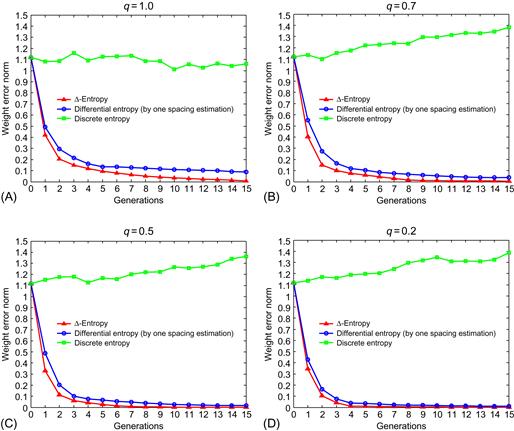
Figure 4.33 Evolution curves of the weight error norm for different entropy criteria (adopted from Ref. [211]).
The second example illustrates that the ![]() -entropy criterion may yield approximately an unbiased solution even if the input and output data are both corrupted by noises. Consider again the identification of a two-tap FIR filter in which
-entropy criterion may yield approximately an unbiased solution even if the input and output data are both corrupted by noises. Consider again the identification of a two-tap FIR filter in which ![]() . We assume the input signal
. We assume the input signal ![]() , input noise
, input noise ![]() , and the output noise
, and the output noise ![]() are all zero-mean white Bernoulli processes with distributions below
are all zero-mean white Bernoulli processes with distributions below
 (4.291)
where ![]() ,
, ![]() , and
, and ![]() denote, respectively, the standard deviations of
denote, respectively, the standard deviations of ![]() ,
, ![]() , and
, and ![]() . In the simulation we set
. In the simulation we set ![]() , and the number of training data is
, and the number of training data is ![]() . Simulation results over 100 Monte Carlo runs are listed in Tables 4.9 and 4.10. For comparison purpose, we also present the results obtained using MSE criterion. As one can see, the
. Simulation results over 100 Monte Carlo runs are listed in Tables 4.9 and 4.10. For comparison purpose, we also present the results obtained using MSE criterion. As one can see, the ![]() -entropy criterion produces nearly unbiased estimates under various SNR conditions, whereas the MSE criterion yields biased solution especially when the input noise power increasing.
-entropy criterion produces nearly unbiased estimates under various SNR conditions, whereas the MSE criterion yields biased solution especially when the input noise power increasing.


4.8 System Identification with MCC
Correntropy is closely related to Renyi’s quadratic entropy. With Gaussian kernel, correntropy is a localized similarity measure between two random variables: when two points are close, the correntropy induced metric (CIM) behaves like an L2 norm; outside of the L2 zone CIM behaves like an L1 norm; as two points are further apart, the metric approaches L0 norm [137]. This property makes the MCC a robust adaptation criterion in presence of non-Gaussian impulsive noise. At the end of this chapter, we briefly discuss the application of the MCC criterion to system identification.
Consider a general scheme of system identification as shown in Figure 4.1. The objective of the identification is to optimize a criterion function (or cost function) in such a way that the model output ![]() resembles as closely as possible the measured output
resembles as closely as possible the measured output ![]() . Under the MCC criterion, the cost function that we want to maximize is the correntropy between the measured output and the model output, i.e.,
. Under the MCC criterion, the cost function that we want to maximize is the correntropy between the measured output and the model output, i.e.,
 (4.292)
In practical applications, one often uses the following empirical correntropy as the cost function:
![]() (4.293)
(4.293)
Then a gradient-based identification algorithm can be easily derived as follows:
![]() (4.294)
(4.294)
When ![]() , the above algorithm becomes a stochastic gradient-based (LMS-like) algorithm:
, the above algorithm becomes a stochastic gradient-based (LMS-like) algorithm:
![]() (4.295)
(4.295)
In the following, we present two simulation examples of FIR identification to demonstrate the performance of MCC criterion, and compare it with the performance of MSE and MEE.
In the first example, the weight vector of the plant is [138]
![]() (4.296)
(4.296)
The input signal is a white Gaussian process with zero mean and unit variance. The noise distribution is a mixture of Gaussian:
![]() (4.297)
(4.297)
In this distribution, the Gaussian density with variance 10 creates strong outliers. The kernel sizes for the MCC and the MEE are set at 2.0. The step-sizes for the three identification criteria are chosen such that when the observation noise is Gaussian, their performance is similar in terms of the weight SNR (WSNR),
![]() (4.298)
(4.298)
Figure 4.34 shows the performance in the presence of impulsive noise. One can see the MCC criterion achieves a more robust performance.

Figure 4.34 WSNR of three identification criteria in impulsive measurement noise (adopted from Ref. [138]).
In the second example, the plant has a time-varying transfer function, where the weight vector is changing as follows [138]:
![]() (4.299)
(4.299)
where ![]() is the unit step function. The simulation results are shown in Figure 4.35. Once again the MCC criterion performs better in impulsive noise environment.
is the unit step function. The simulation results are shown in Figure 4.35. Once again the MCC criterion performs better in impulsive noise environment.

Figure 4.35 WSNR of three identification criteria while tracking a time-varying system in impulsive measurement noise (adopted from Ref. [138]).
Appendix H Vector Gradient and Matrix Gradient
In many of system identification applications, we often encounter a cost function that we want to maximize (or minimize) with respect to a vector or matrix. To accomplish this optimization, we usually need to find a vector or matrix derivative.
Derivative of Scalar with Respect to Vector
If ![]() is a scalar,
is a scalar, ![]() is an
is an ![]() vector, then
vector, then
![]() (H.1)
(H.1)
 (H.2)
(H.2)
Derivative of Scalar with Respect to Matrix
If ![]() is a scalar,
is a scalar, ![]() is an
is an ![]() matrix,
matrix, ![]() , then
, then
 (H.3)
(H.3)


1In the case of black-box identification, the model parameters are basically viewed as vehicles for adjusting the fit to data and do not reflect any physical consideration in the system.
2For a dynamic system, the input vector may contain past inputs and outputs.
3The Mercer theorem states that any reproducing kernel ![]() can be expanded as follows [160]:
can be expanded as follows [160]:
![]()
where ![]() and
and ![]() are the eigenvalues and the eigenfunctions, respectively. The eigenvalues are nonnegative. Therefore, a mapping
are the eigenvalues and the eigenfunctions, respectively. The eigenvalues are nonnegative. Therefore, a mapping ![]() can be constructed as
can be constructed as
![]()
By construction, the dimensionality of ![]() is determined by the number of strictly positive eigenvalues, which can be infinite (e.g., for the Gaussian kernel case).
is determined by the number of strictly positive eigenvalues, which can be infinite (e.g., for the Gaussian kernel case).
4See Appendix H for the calculation of the gradient in vector or matrix form.
5The step-size is critical to the performance of the LMS. In general, the choice of step-size is a trade-off between the convergence rate and the asymptotic EMSE [19,20].
6The LMS algorithm usually assumes an FIR model [19,20].
7In practical applications, if the samples are not i.i.d., the KDE method can still be applied.
8The kernel function for density estimation is not necessarily a Mercer kernel. In this book, to make a distinction between these two types of kernels, we denote them by ![]() and
and ![]() , respectively.
, respectively.
9It should be noted that the error samples at time k are not necessarily to be a tap delayed sequence. A more general expression of the error samples can be ![]() .
.
10Since error entropy is shift-invariant, after training under MEE criterion the bias value of the output PE was adjusted so as to yield zero-mean error over the training set.
11Here the input vector is a row vector.
12This configuration has been widely adopted due to its convenience for convergence analysis (e.g., see Ref. [196]).
13Similar to [29], the subscript ![]() in
in ![]() indicates that the Gaussian assumption A2 is the main assumption leading to the defined expression (4.163). The subscript
indicates that the Gaussian assumption A2 is the main assumption leading to the defined expression (4.163). The subscript ![]() for
for ![]() , which is defined later in (4.166), however, suggests that the independence assumption A4 is the major assumption in evaluating the expectation.
, which is defined later in (4.166), however, suggests that the independence assumption A4 is the major assumption in evaluating the expectation.
14Increasing the sliding data length can improve both convergence speed and steady-state performance, however, this will increase dramatically the computational burden (![]() ).
).
15For the case in which the error distribution is continuous, one can still use the ![]() -entropy as the optimization criterion if classifying the errors into groups and obtaining the quantized data.
-entropy as the optimization criterion if classifying the errors into groups and obtaining the quantized data.
16The truncation selection is a widely used selection method in EDAs. In the truncation selection, individuals are sorted according to their objective function (or fitness function) values and only the best individuals are selected.
17Strictly speaking, the differential entropy criterion is invalid in this example, because the error is discrete-valued. However, in the simulation one can still adopt the empirical differential entropy.