
Information Theoretic Parameter Estimation
Information theory is closely associated with the estimation theory. For example, the maximum entropy (MaxEnt) principle has been widely used to deal with estimation problems given incomplete knowledge or data. Another example is the Fisher information, which is a central concept in statistical estimation theory. Its inverse yields a fundamental lower bound on the variance of any unbiased estimator, i.e., the well-known Cramer–Rao lower bound (CRLB). An interesting link between information theory and estimation theory was also shown for the Gaussian channel, which relates the derivative of the mutual information with the minimum mean square error (MMSE) [81].
3.1 Traditional Methods for Parameter Estimation
Estimation theory is a branch of statistics and signal processing that deals with estimating the unknown values of parameters based on measured (observed) empirical data. Many estimation methods can be found in the literature. In general, the statistical estimation can be divided into two main categories: point estimation and interval estimation. The point estimation involves the use of empirical data to calculate a single value of an unknown parameter, while the interval estimation is the use of empirical data to calculate an interval of possible values of an unknown parameter. In this book, we only discuss the point estimation. The most common approaches to point estimation include the maximum likelihood (ML), method of moments (MM), MMSE (also known as Bayes least squared error), maximum a posteriori (MAP), and so on. These estimation methods also fall into two categories, namely, classical estimation (ML, MM, etc.) and Bayes estimation (MMSE, MAP, etc.).
3.1.1 Classical Estimation
The general description of the classical estimation is as follows: let the distribution function of population ![]() be
be ![]() , where
, where ![]() is an unknown (but deterministic) parameter that needs to be estimated. Suppose
is an unknown (but deterministic) parameter that needs to be estimated. Suppose ![]() are samples (usually independent and identically distributed, i.i.d.) coming from
are samples (usually independent and identically distributed, i.i.d.) coming from ![]() (
(![]() are corresponding sample values). Then the goal of estimation is to construct an appropriate statistics
are corresponding sample values). Then the goal of estimation is to construct an appropriate statistics ![]() that serves as an approximation of unknown parameter
that serves as an approximation of unknown parameter ![]() . The statistics
. The statistics ![]() is called an estimator of
is called an estimator of ![]() , and its sample value
, and its sample value ![]() is called the estimated value of
is called the estimated value of ![]() . Both the samples
. Both the samples ![]() and the parameter
and the parameter ![]() can be vectors.
can be vectors.
The ML estimation and the MM are two prevalent types of classical estimation.
3.1.1.1 ML Estimation
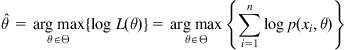
The ML method, proposed by the famous statistician R.A. Fisher, leads to many well-known estimation methods in statistics. The basic idea of ML method is quite simple: the event with greatest probability is most likely to occur. Thus, one should choose the parameter that maximizes the probability of the observed sample data. Assume that ![]() is a continuous random variable with probability density function (PDF)
is a continuous random variable with probability density function (PDF) ![]() ,
, ![]() , where
, where ![]() is an unknown parameter,
is an unknown parameter, ![]() is the set of all possible parameters. The ML estimate of parameter
is the set of all possible parameters. The ML estimate of parameter ![]() is expressed as
is expressed as
![]() (3.1)
(3.1)
where ![]() is the joint PDF of samples
is the joint PDF of samples ![]() . By considering the sample values
. By considering the sample values ![]() to be fixed “parameters,” this joint PDF is a function of the parameter
to be fixed “parameters,” this joint PDF is a function of the parameter ![]() , called the likelihood function, denoted by
, called the likelihood function, denoted by ![]() . If samples
. If samples ![]() are i.i.d., we have
are i.i.d., we have ![]() . Then the ML estimate of
. Then the ML estimate of ![]() becomes
becomes
![]() (3.2)
(3.2)
In practice, it is often more convenient to work with the logarithm of the likelihood function (called the log-likelihood function). In this case, we have
 (3.3)
(3.3)
An ML estimate is the same regardless of whether we maximize the likelihood or log-likelihood function, since log is a monotone transformation.
In most cases, the ML estimate can be solved by setting the derivative of the log-likelihood function to zero:
![]() (3.4)
(3.4)
For many models, however, there is no closed form solution of ML estimate, and it has to be found numerically using optimization methods.
If the likelihood function involves latent variables in addition to unknown parameter ![]() and known data observations
and known data observations ![]() , one can use the expectation–maximization (EM) algorithm to find the ML solution [164,165] (see Appendix E). Typically, the latent variables are included in a likelihood function because either there are missing values among the data or the model can be formulated more simply by assuming the existence of additional unobserved data points.
, one can use the expectation–maximization (EM) algorithm to find the ML solution [164,165] (see Appendix E). Typically, the latent variables are included in a likelihood function because either there are missing values among the data or the model can be formulated more simply by assuming the existence of additional unobserved data points.
ML estimators possess a number of attractive properties especially when sample size tends to infinity. In general, they have the following properties:
• Consistency: As the sample size increases, the estimator converges in probability to the true value being estimated.
• Asymptotic normality: As the sample size increases, the distribution of the estimator tends to the Gaussian distribution.
• Efficiency: The estimator achieves the CRLB when the sample size tends to infinity.
3.1.1.2 Method of Moments
The MM uses the sample algebraic moments to approximate the population algebraic moments, and then solves the parameters. Consider a continuous random variable ![]() , with PDF
, with PDF ![]() , where
, where ![]() are
are ![]() unknown parameters. By the law of large numbers, the
unknown parameters. By the law of large numbers, the ![]() -order sample moment
-order sample moment ![]() of
of ![]() will converge in probability to the
will converge in probability to the ![]() -order population moment
-order population moment ![]() , which is a function of
, which is a function of ![]() , i.e.,
, i.e.,
![]() (3.5)
(3.5)
The sample moment ![]() is a good approximation of the population moment
is a good approximation of the population moment ![]() , thus one can achieve an estimator of parameters
, thus one can achieve an estimator of parameters ![]() (
(![]() ) by solving the following equations:
) by solving the following equations:
 (3.6)
(3.6)
The solution of (3.6) is the MM estimator, denoted by ![]() ,
, ![]() .
.
3.1.2 Bayes Estimation
The basic viewpoint of Bayes statistics is that in any statistic reasoning problem, a prior distribution must be prescribed as a basic factor in the reasoning process, besides the availability of empirical data. Unlike classical estimation, the Bayes estimation regards the unknown parameter as a random variable (or random vector) with some prior distribution. In many situations, this prior distribution does not need to be precise, which can be even improper (e.g., uniform distribution on the whole space). Since the unknown parameter is a random variable, in the following we use ![]() to denote the parameter to be estimated, and
to denote the parameter to be estimated, and ![]() to denote the observation data
to denote the observation data ![]() .
.
Assume that both the parameter ![]() and observation
and observation ![]() are continuous random variables with joint PDF
are continuous random variables with joint PDF
![]() (3.7)
(3.7)
where ![]() is the marginal PDF of
is the marginal PDF of ![]() (the prior PDF) and
(the prior PDF) and ![]() is the conditional PDF of
is the conditional PDF of ![]() given
given ![]() (also known as the likelihood function if considering
(also known as the likelihood function if considering ![]() as the function’s variable). By using the Bayes formula, one can obtain the posterior PDF of
as the function’s variable). By using the Bayes formula, one can obtain the posterior PDF of ![]() given
given ![]() :
:
![]() (3.8)
(3.8)
Let ![]() be an estimator of
be an estimator of ![]() (based on the observation
(based on the observation ![]() ), and let
), and let ![]() be a loss function that measures the difference between random variables
be a loss function that measures the difference between random variables ![]() and
and ![]() . The Bayes risk of
. The Bayes risk of ![]() is defined as the expected loss (the expectation is taken over the joint distribution of
is defined as the expected loss (the expectation is taken over the joint distribution of ![]() and
and ![]() ):
):
 (3.9)
(3.9)
where ![]() denotes the posterior expected loss (posterior Bayes risk). An estimator is said to be a Bayes estimator if it minimizes the Bayes risk among all estimators. Thus, the Bayes estimator can be obtained by solving the following optimization problem:
denotes the posterior expected loss (posterior Bayes risk). An estimator is said to be a Bayes estimator if it minimizes the Bayes risk among all estimators. Thus, the Bayes estimator can be obtained by solving the following optimization problem:
![]() (3.10)
(3.10)
where ![]() denotes all Borel measurable functions
denotes all Borel measurable functions ![]() . Obviously, the Bayes estimator also minimizes the posterior Bayes risk for each
. Obviously, the Bayes estimator also minimizes the posterior Bayes risk for each ![]() .
.
The loss function in Bayes risk is usually a function of the estimation error ![]() . The common loss functions used for Bayes estimation include:
. The common loss functions used for Bayes estimation include:
3. 0–1 loss function: ![]() , where
, where ![]() denotes the delta function.1
denotes the delta function.1
The squared error loss corresponds to the MSE criterion, which is perhaps the most prevalent risk function in use due to its simplicity and efficiency. With the above loss functions, the Bayes estimates of the unknown parameter are, respectively, the mean, median, and mode2 of the posterior PDF ![]() , i.e.,
, i.e.,
 (3.11)
The estimators (a) and (c) in (3.11) are known as the MMSE and MAP estimators. A simple proof of the MMSE estimator is given in Appendix F. It should be noted that if the posterior PDF is symmetric and unimodal (SUM, such as Gaussian distribution), the three Bayes estimators are identical.
The MAP estimate is a mode of the posterior distribution. It is a limit of Bayes estimation under 0–1 loss function. When the prior distribution is uniform (i.e., a constant function), the MAP estimation coincides with the ML estimation. Actually, in this case we have
 (3.12)
where (a) comes from the fact that ![]() is a constant.
is a constant.
Besides the previous common risks, other Bayes risks can be conceived. Important examples include the mean ![]() -power error [30], Huber’s M-estimation cost [33], and the risk-sensitive cost [38], etc. It has been shown in [24] that if the posterior PDF is symmetric, the posterior mean is an optimal estimate for a large family of Bayes risks, where the loss function is even and convex.
-power error [30], Huber’s M-estimation cost [33], and the risk-sensitive cost [38], etc. It has been shown in [24] that if the posterior PDF is symmetric, the posterior mean is an optimal estimate for a large family of Bayes risks, where the loss function is even and convex.
In general, a Bayes estimator is a nonlinear function of the observation. However, if ![]() and
and ![]() are jointly Gaussian, then the MMSE estimator is linear. Suppose
are jointly Gaussian, then the MMSE estimator is linear. Suppose ![]() ,
, ![]() , with jointly Gaussian PDF
, with jointly Gaussian PDF
 (3.13)
where ![]() is the covariance matrix:
is the covariance matrix:
![]() (3.14)
(3.14)
Then the posterior PDF ![]() is also Gaussian and has mean (the MMSE estimate)
is also Gaussian and has mean (the MMSE estimate)
![]() (3.15)
(3.15)
which is, obviously, a linear function of ![]() .
.
There are close relationships between estimation theory and information theory. The concepts and principles in information theory can throw new light on estimation problems and suggest new methods for parameter estimation. In the sequel, we will discuss information theoretic approaches to parameter estimation.
3.2 Information Theoretic Approaches to Classical Estimation
In the literature, there have been many reports on the use of information theory to deal with classical estimation problems (e.g., see [149]). Here, we only give several typical examples.
3.2.1 Entropy Matching Method
Similar to the MM, the entropy matching method obtains the parameter estimator by using the sample entropy (entropy estimator) to approximate the population entropy. Suppose the PDF of population ![]() is
is ![]() (
(![]() is an unknown parameter). Then its differential entropy is
is an unknown parameter). Then its differential entropy is
![]() (3.16)
(3.16)
At the same time, one can use the sample ![]() to calculate the sample entropy
to calculate the sample entropy ![]() .3 Thus, we can obtain an estimator of parameter
.3 Thus, we can obtain an estimator of parameter ![]() through solving the following equation:
through solving the following equation:
![]() (3.17)
(3.17)
If there are several parameters, the above equation may have infinite number of solutions, while a unique solution can be achieved by combining the MM. In [166], the entropy matching method was used to estimate parameters of generalized Gaussian distribution (GGD).
3.2.2 Maximum Entropy Method
The maximum entropy method applies the famous MaxEnt principle to parameter estimation. The basic idea is that, subject to the information available, one should choose the parameter ![]() such that the entropy is as large as possible, or the distribution as nearly uniform as possible. Here, the maximum entropy method refers to a general approach rather than a specific parameter estimation method. In the following, we give three examples of maximum entropy method.
such that the entropy is as large as possible, or the distribution as nearly uniform as possible. Here, the maximum entropy method refers to a general approach rather than a specific parameter estimation method. In the following, we give three examples of maximum entropy method.
3.2.2.1 Parameter Estimation of Exponential Type Distribution
Assume that the PDF of population ![]() is of the following form:
is of the following form:
 (3.18)
where ![]() ,
, ![]() , are
, are ![]() (generalized) characteristic moment functions,
(generalized) characteristic moment functions, ![]() is an unknown parameter vector to be estimated. Many known probability distributions are special cases of this exponential type distribution. By Theorem 2.2,
is an unknown parameter vector to be estimated. Many known probability distributions are special cases of this exponential type distribution. By Theorem 2.2, ![]() is the maximum entropy distribution satisfying the following constraints:
is the maximum entropy distribution satisfying the following constraints:
![]() (3.19)
(3.19)
where ![]() denotes the population characteristic moment:
denotes the population characteristic moment:
![]() (3.20)
(3.20)
As ![]() is unknown, the population characteristic moments cannot be calculated. We can approximate them using the sample characteristic moments. And then, an estimator of parameter
is unknown, the population characteristic moments cannot be calculated. We can approximate them using the sample characteristic moments. And then, an estimator of parameter ![]() can be obtained by solving the following optimization problem:
can be obtained by solving the following optimization problem:
 (3.21)
where ![]() ,
, ![]() , are
, are ![]() sample characteristic moments, i.e.,
sample characteristic moments, i.e.,
![]() (3.22)
(3.22)
According to Theorem 2.2, the estimator of ![]() satisfies the equations:
satisfies the equations:
 (3.23)
If ![]() , the above estimation method will be equivalent to the MM.
, the above estimation method will be equivalent to the MM.
3.2.2.2 Maximum Spacing Estimation
Suppose the distribution function of population ![]() is
is ![]() , and the true value of the unknown parameter
, and the true value of the unknown parameter ![]() is
is ![]() , then the random variable
, then the random variable ![]() will be distributed over the interval
will be distributed over the interval ![]() , which is a uniform distribution if
, which is a uniform distribution if ![]() . According to the MaxEnt principle, if the distribution over a finite interval is uniform, the entropy will achieve its maximum. Therefore, the entropy of random variable
. According to the MaxEnt principle, if the distribution over a finite interval is uniform, the entropy will achieve its maximum. Therefore, the entropy of random variable ![]() will attain the maximum value if
will attain the maximum value if ![]() . So one can obtain an estimator of the parameter
. So one can obtain an estimator of the parameter ![]() by maximizing the sample entropy of
by maximizing the sample entropy of ![]() . Let a sample of population
. Let a sample of population ![]() be
be ![]() , the sample of
, the sample of ![]() will be
will be ![]() . Let
. Let ![]() denote the sample entropy of
denote the sample entropy of ![]() , the estimator of parameter
, the estimator of parameter ![]() can be expressed as
can be expressed as
![]() (3.24)
(3.24)
If the sample entropy is calculated by using the one-spacing estimation method (see Chapter 4), then we have
![]() (3.25)
(3.25)
where ![]() is the order statistics of
is the order statistics of ![]() . Formula (3.25) is called the maximum spacing estimation of parameter
. Formula (3.25) is called the maximum spacing estimation of parameter ![]() .
.
3.2.2.3 Maximum Equality Estimation
Suppose ![]() is an i.i.d. sample of population
is an i.i.d. sample of population ![]() with PDF
with PDF ![]() . Let
. Let ![]() be the order statistics of
be the order statistics of ![]() . Then the random sample divides the real axis into
. Then the random sample divides the real axis into ![]() subintervals
subintervals ![]() ,
, ![]() , where
, where ![]() and
and ![]() . Each subinterval has the probability:
. Each subinterval has the probability:
![]() (3.26)
(3.26)
Since the sample is random and i.i.d., the most reasonable situation is that the probabilities of ![]() subinterval are equal. Hence, the parameter
subinterval are equal. Hence, the parameter ![]() should be chosen in such a way as to maximize the entropy of distribution
should be chosen in such a way as to maximize the entropy of distribution ![]() (or to make
(or to make ![]() as nearly uniform as possible), i.e.,
as nearly uniform as possible), i.e.,
 (3.27)
The above estimation is called the maximum equality estimation of parameter ![]() .
.
It is worth noting that besides parameter estimation, the MaxEnt principle can also be applied to spectral density estimation [48]. The general idea is that the maximum entropy rate stochastic process that satisfies the given constant autocorrelation and variance constraints, is a linear Gauss–Markov process with i.i.d. zero-mean, Gaussian input.
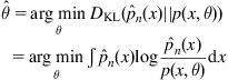
3.2.3 Minimum Divergence Estimation
Let ![]() be an i.i.d. random sample from a population
be an i.i.d. random sample from a population ![]() with PDF
with PDF ![]() ,
, ![]() . Let
. Let ![]() be the estimated PDF based on the sample. Let
be the estimated PDF based on the sample. Let ![]() be an estimator of
be an estimator of ![]() . Then
. Then ![]() is also an estimator for
is also an estimator for ![]() . Then the estimator
. Then the estimator ![]() should be chosen so that
should be chosen so that ![]() is as close as possible to
is as close as possible to ![]() . This can be achieved by minimizing any measure of information divergence, say the KL-divergence
. This can be achieved by minimizing any measure of information divergence, say the KL-divergence
 (3.28)
or, alternatively,
 (3.29)
The estimate ![]() in (3.28) or (3.29) is called the minimum divergence (MD) estimate of
in (3.28) or (3.29) is called the minimum divergence (MD) estimate of ![]() . In practice, we usually use (3.28) for parameter estimation, because it can be simplified as
. In practice, we usually use (3.28) for parameter estimation, because it can be simplified as
![]() (3.30)
(3.30)
Depending on the estimated PDF ![]() , the MD estimator may take many different forms. Next, we present three specific examples of MD estimator.
, the MD estimator may take many different forms. Next, we present three specific examples of MD estimator.
• MD Estimator 1
Without loss of generality, we assume that the sample satisfies ![]() . Then the distribution function can be estimated as
. Then the distribution function can be estimated as
 (3.31)
 (3.32)
where ![]() is the likelihood function. In this case, the MD estimation is exactly the ML estimation.
is the likelihood function. In this case, the MD estimation is exactly the ML estimation.
• MD Estimator 2
Suppose the population ![]() is distributed over the interval
is distributed over the interval ![]() , and the sample satisfies
, and the sample satisfies ![]() . It is reasonable to assume that in each subinterval
. It is reasonable to assume that in each subinterval ![]() , the probability is
, the probability is ![]() . And hence, the PDF of
. And hence, the PDF of ![]() can be estimated as
can be estimated as
![]() (3.33)
(3.33)
Substituting (3.33) into (3.30) yields
 (3.34)
If ![]() is a continuous function of
is a continuous function of ![]() , then according to the mean value theorem of integral calculus, we have
, then according to the mean value theorem of integral calculus, we have
![]() (3.35)
(3.35)
where ![]() . Hence, (3.34) can be written as
. Hence, (3.34) can be written as
![]() (3.36)
(3.36)
The above parameter estimation is in form very similar to the ML estimation. However, different from Fisher’s likelihood function, the values of the cost function in (3.36) are taken at ![]() , which are determined by mean value theorem of integral calculus.
, which are determined by mean value theorem of integral calculus.
• MD Estimator 3
Assume population ![]() is distributed over the interval
is distributed over the interval ![]() , and this interval is divided into
, and this interval is divided into ![]() subintervals
subintervals ![]() (
(![]() ) by
) by ![]() data
data ![]() . The probability of each subinterval is determined by
. The probability of each subinterval is determined by
![]() (3.37)
(3.37)
If ![]() are given proportions of the population that lie in the
are given proportions of the population that lie in the ![]() subintervals (
subintervals (![]() ), then parameter
), then parameter ![]() should be chosen so as to make
should be chosen so as to make ![]() and
and ![]() as close as possible, i.e.,
as close as possible, i.e.,
 (3.38)
This is a useful estimation approach, especially when the information available is on proportions in the population, such as proportions of persons in different income intervals or proportions of students in different score intervals.
In the previous MD estimations, the KL-divergence can be substituted by other definitions of divergence. For instance, if using ![]() -divergence, we have
-divergence, we have
![]() (3.39)
(3.39)
or
![]() (3.40)
(3.40)
For details on the minimum ![]() -divergence estimation, the readers can refer to [130].
-divergence estimation, the readers can refer to [130].
3.3 Information Theoretic Approaches to Bayes Estimation
The Bayes estimation can also be embedded within the framework of information theory. In particular, some information theoretic measures, such as the entropy and correntropy, can be used instead of the traditional Bayes risks.
3.3.1 Minimum Error Entropy Estimation
In the scenario of Bayes estimation, the minimum error entropy (MEE) estimation aims to minimize the entropy of the estimation error, and hence decrease the uncertainty in estimation. Given two random variables: ![]() , an unknown parameter to be estimated, and
, an unknown parameter to be estimated, and ![]() , the observation (or measurement), the MEE (with Shannon entropy) estimation of
, the observation (or measurement), the MEE (with Shannon entropy) estimation of ![]() based on
based on ![]() can be formulated as
can be formulated as
 (3.41)
where ![]() is the estimation error,
is the estimation error, ![]() is an estimator of
is an estimator of ![]() based on
based on ![]() ,
, ![]() is a measurable function,
is a measurable function, ![]() stands for the collection of all measurable functions
stands for the collection of all measurable functions ![]() , and
, and ![]() denotes the PDF of the estimation error. When (3.41) is compared with (3.9) one concludes that the “loss function” in MEE is
denotes the PDF of the estimation error. When (3.41) is compared with (3.9) one concludes that the “loss function” in MEE is ![]() , which is different from traditional Bayesian risks, like MSE. Indeed one does not need to impose a risk functional in MEE, the risk is directly related to the error PDF. Obviously, other entropy definitions (such as order-
, which is different from traditional Bayesian risks, like MSE. Indeed one does not need to impose a risk functional in MEE, the risk is directly related to the error PDF. Obviously, other entropy definitions (such as order-![]() Renyi entropy) can also be used in MEE estimation. This feature is potentially beneficial because the risk is matched to the error distribution.
Renyi entropy) can also be used in MEE estimation. This feature is potentially beneficial because the risk is matched to the error distribution.
The early work in MEE estimation can be traced back to the late 1960s when Weidemann and Stear [86] studied the use of error entropy as a criterion function (risk function) for analyzing the performance of sampled data estimation systems. They proved that minimizing the error entropy is equivalent to minimizing the mutual information between the error and the observation, and also proved that the reduced error entropy is upper-bounded by the amount of information obtained by the observation. Minamide [89] extended Weidemann and Stear’s results to a continuous-time estimation system. Tomita et al. applied the MEE criterion to linear Gaussian systems and studied state estimation (Kalman filtering), smoothing, and predicting problems from the information theory viewpoint. In recent years, the MEE became an important criterion in supervised machine learning [64].
In the following, we present some important properties of the MEE criterion, and discuss its relationship to conventional Bayes risks. For simplicity, we assume that the error ![]() is a scalar (
is a scalar (![]() ). The extension to arbitrary dimensions will be straightforward.
). The extension to arbitrary dimensions will be straightforward.
3.3.1.1 Some Properties of MEE Criterion
Property 1:
![]() ,
, ![]()
Proof:
This is the shift invariance of the differential entropy. According to the definition of differential entropy, we have
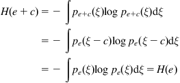 (3.42)
Property 2:
If ![]() is a random variable independent of the error
is a random variable independent of the error ![]() , then
, then ![]() .
.
Proof:
According to the properties of differential entropy and the independence condition, we have
![]() (3.43)
(3.43)
Remark:
Property 2 implies that MEE criterion is robust to independent additive noise. Specifically, if error ![]() contains an independent additive noise
contains an independent additive noise ![]() , i.e.,
, i.e., ![]() , where
, where ![]() is the true error, then minimizing the contaminated error entropy
is the true error, then minimizing the contaminated error entropy ![]() will constrain the true error entropy
will constrain the true error entropy ![]() .
.
Property 3:
Minimizing the error entropy ![]() is equivalent to minimizing the mutual information between error
is equivalent to minimizing the mutual information between error ![]() and the observation
and the observation ![]() , i.e.,
, i.e., ![]() .
.
Proof:
As ![]() , we have
, we have
 (3.44)
It follows easily that
 (3.45)
where (a) comes from the fact that the conditional entropy ![]() is not related to
is not related to ![]() .
.
Property 4:
The error entropy ![]() is lower bounded by the conditional entropy
is lower bounded by the conditional entropy ![]() , and this lower bound is achieved if and only if error
, and this lower bound is achieved if and only if error ![]() is independent of the observation
is independent of the observation ![]() .
.
Proof:
By (3.44), we have
![]() (3.46)
(3.46)
where the inequality follows from the fact that ![]() , with equality if and only if error
, with equality if and only if error ![]() and observation
and observation ![]() are independent.
are independent.
Remark:
The error entropy can never be smaller than the conditional entropy of the parameter ![]() given observation
given observation ![]() . This lower bound is achieved if and only if the error contains no information about the observation.
. This lower bound is achieved if and only if the error contains no information about the observation.
For MEE estimation, there is no explicit expression for the optimal estimate unless some constraints on the posterior PDF are imposed. The next property shows that, if the posterior PDF is SUM, the MEE estimate will be equal to the conditional mean (i.e., the MMSE estimate).
Property 5:
If for any ![]() , the posterior PDF
, the posterior PDF ![]() is SUM, then the MEE estimate equals the posterior mean, i.e.,
is SUM, then the MEE estimate equals the posterior mean, i.e., ![]() .
.
Remark:
Since the posterior PDF is SUM, in the above property the MEE estimate also equals the posterior median or posterior mode. We point out that for order-![]() Renyi entropy, this property still holds. One may be led to conclude that MEE has no advantage over the MMSE, since they correspond to the same solution for SUM case. However, the risk functional in MEE is still well defined for unimodal but asymmetric distributions, although no general results are known for this class of distributions. But we suspect that the practical advantages of MEE versus MSE reported in the literature [64] are taking advantage of this case. In the context of adaptive filtering, the two criteria may yield much different performance surfaces even if they have the same optimal solution.
Renyi entropy, this property still holds. One may be led to conclude that MEE has no advantage over the MMSE, since they correspond to the same solution for SUM case. However, the risk functional in MEE is still well defined for unimodal but asymmetric distributions, although no general results are known for this class of distributions. But we suspect that the practical advantages of MEE versus MSE reported in the literature [64] are taking advantage of this case. In the context of adaptive filtering, the two criteria may yield much different performance surfaces even if they have the same optimal solution.
Table 3.1 gives a summary of the optimal estimates for several Bayes estimation methods.

Proof:
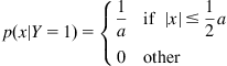
We prove this property by means of a simple example as follows [94]: suppose ![]() is a discrete random variable with Bernoulli distribution:
is a discrete random variable with Bernoulli distribution:
![]() (3.47)
(3.47)
The posterior PDF of ![]() given
given ![]() is (
is (![]() ):
):

Given an estimator ![]() , the error PDF will be
, the error PDF will be
![]() (3.48)
(3.48)
Let ![]() be an unbiased estimator, then
be an unbiased estimator, then ![]() , and hence
, and hence ![]() . Assuming
. Assuming ![]() (due to symmetry, one can obtain similar results for
(due to symmetry, one can obtain similar results for ![]() ), the error entropy can be calculated as
), the error entropy can be calculated as
 (3.49)
One can easily verify that the error entropy achieves its minimum value when ![]() . Clearly, in this example there are infinitely many unbiased MEE estimators.
. Clearly, in this example there are infinitely many unbiased MEE estimators.
Property 7 (Score Orthogonality [92]):
Given an MEE estimator ![]() , the error’s score
, the error’s score ![]() is orthogonal to any measurable function
is orthogonal to any measurable function ![]() of
of ![]() , where
, where ![]() is defined as
is defined as
![]() (3.50)
(3.50)
where ![]() denotes the error PDF for estimator
denotes the error PDF for estimator ![]() .
.
Proof:
Given an MEE estimator ![]() ,
, ![]() and
and![]() , we have
, we have
![]() (3.51)
(3.51)
For ![]() small enough,
small enough, ![]() will be a “small” random variable. According to [167], we have
will be a “small” random variable. According to [167], we have
![]() (3.52)
(3.52)
where ![]() denotes the higher order terms. Then the derivative of entropy
denotes the higher order terms. Then the derivative of entropy ![]() with respect to
with respect to ![]() at
at ![]() is
is
![]() (3.53)
(3.53)
Combining (3.51) and (3.53) yields
![]() (3.54)
(3.54)
Remark:
If the error is zero-mean Gaussian distributed with variance ![]() , the score function will be
, the score function will be ![]() . In this case, the score orthogonality condition reduces to
. In this case, the score orthogonality condition reduces to ![]() . This is the well-known orthogonality condition for MMSE estimation.
. This is the well-known orthogonality condition for MMSE estimation.
In MMSE estimation, the orthogonality condition is a necessary and sufficient condition for optimality, and can be used to find the MMSE estimator. In MEE estimation, however, the score orthogonality condition is just a necessary condition for optimality but not a sufficient one. Next, we will present an example to demonstrate that if an estimator satisfies the score orthogonality condition, it can be a local minimum or even a local maximum of ![]() in a certain direction. Before proceeding, we give a definition.
in a certain direction. Before proceeding, we give a definition.
Definition 3.1
Given an estimator ![]() ,
, ![]() is said to be a local minimum (or maximum) of
is said to be a local minimum (or maximum) of ![]() in the direction of
in the direction of ![]() , if and only if
, if and only if ![]() , such that
, such that ![]() ,
, ![]() , we have
, we have
![]() (3.55)
(3.55)
Example 3.1 [92]
Suppose the joint PDF of ![]() and
and ![]() is the mix-Gaussian density (
is the mix-Gaussian density (![]() ):
):
 (3.56)
The MMSE estimation of ![]() based on
based on ![]() can be computed as
can be computed as ![]() . It is easy to check that the estimator
. It is easy to check that the estimator ![]() satisfies the score orthogonality condition.
satisfies the score orthogonality condition.
Now we examine whether the MMSE estimator ![]() is a local minimum or maximum of the error entropy
is a local minimum or maximum of the error entropy ![]() in a certain direction
in a certain direction ![]() . We focus here on the case where
. We focus here on the case where ![]() (linear function). In this case, we have
(linear function). In this case, we have
![]() (3.57)
(3.57)
For the case ![]() , the error’s entropies
, the error’s entropies ![]() with respect to different
with respect to different ![]() and
and ![]() values are shown in Figure 3.1, from which we see that the MMSE estimator (
values are shown in Figure 3.1, from which we see that the MMSE estimator (![]() ) is a local minimum of the error entropy in the direction of
) is a local minimum of the error entropy in the direction of ![]() for
for ![]() and a local maximum for
and a local maximum for ![]() . In addition, for the case
. In addition, for the case ![]() , the error’s entropies
, the error’s entropies ![]() with respect to different
with respect to different ![]() and
and ![]() values are depicted in Figure 3.2. It can be seen from Figure 3.2 that when
values are depicted in Figure 3.2. It can be seen from Figure 3.2 that when ![]() ,
, ![]() is a global minimum of
is a global minimum of ![]() ; while when
; while when ![]() , it becomes a local maximum.
, it becomes a local maximum.

Figure 3.1 Error’s entropy ![]() with respect to different
with respect to different ![]() and
and ![]() values. Source: Adopted from [92].
values. Source: Adopted from [92].

Figure 3.2 Error’s entropy ![]() with respect to different
with respect to different ![]() and
and ![]() values. Source: Adopted from [92].
values. Source: Adopted from [92].
The local minima or local maxima can also be judged using the second-order derivative of error entropy with respect to ![]() . For instance, if
. For instance, if ![]() , we can calculate the following second-order derivative using results of [167]:
, we can calculate the following second-order derivative using results of [167]:
 (3.58)
And hence
 (3.59)
which implies that if ![]() , the MMSE estimator (
, the MMSE estimator (![]() ) will be a local minimum of the error entropy in the direction of
) will be a local minimum of the error entropy in the direction of ![]() , whereas if
, whereas if ![]() , it becomes a local maximum.
, it becomes a local maximum.
As can be seen from Figure 3.2, if ![]() , the error entropy
, the error entropy ![]() achieves its global minima at
achieves its global minima at ![]() . Figure 3.3 depicts the error PDF for
. Figure 3.3 depicts the error PDF for ![]() (MMSE estimator) and
(MMSE estimator) and ![]() (linear MEE estimator), where
(linear MEE estimator), where ![]() . We can see that the MEE solution is in this case not unique but it is much more concentrated (with higher peak) than the MMSE solution, which potentially gives an estimator with much smaller variance. We can also observe that the peaks of the MMSE and MEE error distributions occur at two different error locations, which means that the best parameter sets are different for each case.
. We can see that the MEE solution is in this case not unique but it is much more concentrated (with higher peak) than the MMSE solution, which potentially gives an estimator with much smaller variance. We can also observe that the peaks of the MMSE and MEE error distributions occur at two different error locations, which means that the best parameter sets are different for each case.

Figure 3.3 Error’s PDF ![]() for
for ![]() and
and ![]() . Source: Adopted from [92].
. Source: Adopted from [92].
3.3.1.2 Relationship to Conventional Bayes Risks
The loss function of MEE criterion is directly related to the error’s PDF, which is much different from the loss functions in conventional Bayes risks, because the user does not need to select the risk functional. To some extent, the error entropy can be viewed as an “adaptive” Bayes risk, in which the loss function is varying with the error distribution, that is, different error distributions correspond to different loss functions. Figure 3.4 shows the loss functions (the lower subplots) of MEE corresponding to three different error PDFs. Notice that the third case provides a risk function that is nonconvex in the space of the errors. This is an unconventional risk function because the role of the weight function is to privilege one solution versus all others in the space of the errors.

There is an important relationship between the MEE criterion and the traditional MSE criterion. The following theorem shows that the MSE is equivalent to the error entropy plus the KL-divergence between the error PDF and any zero-mean Gaussian density.
Theorem 3.1
Let ![]() denote a Gaussian density,
denote a Gaussian density, ![]() , where
, where ![]() . Then we have
. Then we have
![]() (3.60)
(3.60)
Proof:
Since ![]() , we have
, we have
![]()
And hence
 (3.61)
It follows easily that ![]() .
.
Remark:
The above theorem suggests that the minimization of MSE minimizes both the error entropy ![]() and the KL-divergence
and the KL-divergence ![]() . Then the MMSE estimation will decrease the error entropy, and at the same time, make the error distribution close to zero-mean Gaussian distribution. In nonlinear and non-Gaussian estimating systems, the desirable error distribution can be far from Gaussian, while the MSE criterion still makes the error distribution close to zero-mean Gaussian distribution, which may lead to poor estimation performance. Thus, Theorem 3.1 also gives an explanation on why the performance of MMSE estimation may be not good for non-Gaussian samples.
. Then the MMSE estimation will decrease the error entropy, and at the same time, make the error distribution close to zero-mean Gaussian distribution. In nonlinear and non-Gaussian estimating systems, the desirable error distribution can be far from Gaussian, while the MSE criterion still makes the error distribution close to zero-mean Gaussian distribution, which may lead to poor estimation performance. Thus, Theorem 3.1 also gives an explanation on why the performance of MMSE estimation may be not good for non-Gaussian samples.
Suppose that the error is zero-mean Gaussian distributed. Then we have ![]() , where
, where ![]() . In this case, the MSE criterion is equivalent to the MEE criterion.
. In this case, the MSE criterion is equivalent to the MEE criterion.
From the derivation of Theorem 3.1, let ![]() , we have
, we have
![]() (3.62)
(3.62)
Since ![]() , then
, then
![]() (3.63)
(3.63)
Inequality (3.63) suggests that, minimizing the MSE is equivalent to minimizing an upper bound of error entropy.
There exists a similar relationship between MEE criterion and a large family of Bayes risks [168]. To prove this fact, we need a lemma.
Theorem 3.2
For any Bayes risk ![]() , if the loss function
, if the loss function ![]() satisfies
satisfies ![]() , then
, then
![]() (3.66)
(3.66)
where ![]() is the PDF given in (3.64).
is the PDF given in (3.64).
Proof:
First, we show that in the PDF ![]() ,
, ![]() is a positive number. Since
is a positive number. Since ![]() satisfies
satisfies ![]() and
and ![]() , we have
, we have ![]() . Then
. Then
 (3.67)
where (a) follows from ![]() . Therefore,
. Therefore,
 (3.68)
which completes the proof.
Remark:
The condition ![]() in the theorem is not very restrictive, because for most Bayes risks, the loss function increases rapidly when
in the theorem is not very restrictive, because for most Bayes risks, the loss function increases rapidly when ![]() goes to infinity. But for instance, it does not apply to the maximum correntropy (MC) criterion studied next.
goes to infinity. But for instance, it does not apply to the maximum correntropy (MC) criterion studied next.
3.3.2 MC Estimation
Correntropy is a novel measure of similarity between two random variables [64]. Let ![]() and
and ![]() be two random variables with the same dimensions, the correntropy is
be two random variables with the same dimensions, the correntropy is
![]() (3.69)
(3.69)
where ![]() is a translation invariant Mercer kernel. The most popular kernel used in correntropy is the Gaussian kernel:
is a translation invariant Mercer kernel. The most popular kernel used in correntropy is the Gaussian kernel:
![]() (3.70)
(3.70)
where ![]() denotes the kernel size (kernel width). Gaussian kernel
denotes the kernel size (kernel width). Gaussian kernel ![]() is a translation invariant kernel that is a function of
is a translation invariant kernel that is a function of ![]() , so it can be rewritten as
, so it can be rewritten as ![]() .
.
Compared with other similarity measures, such as the mean square error, correntropy (with Gaussian kernel) has some nice properties: (i) it is always bounded (![]() ); (ii) it contains all even-order moments of the difference variable for the Gaussian kernel (using a series expansion); (iii) the weights of higher order moments are controlled by kernel size; and (iv) it is a local similarity measure, and is very robust to outliers.
); (ii) it contains all even-order moments of the difference variable for the Gaussian kernel (using a series expansion); (iii) the weights of higher order moments are controlled by kernel size; and (iv) it is a local similarity measure, and is very robust to outliers.
The correntropy function can also be applied to Bayes estimation [169]. Let ![]() be an unknown parameter to be estimated and
be an unknown parameter to be estimated and ![]() be the observation. We assume, for simplification, that
be the observation. We assume, for simplification, that ![]() is a scalar random variable (extension to the vector case is straightforward),
is a scalar random variable (extension to the vector case is straightforward), ![]() , and
, and ![]() is a random vector taking values in
is a random vector taking values in ![]() . The MC estimation of
. The MC estimation of ![]() based on
based on ![]() is to find a measurable function
is to find a measurable function ![]() such that the correntropy between
such that the correntropy between ![]() and
and ![]() is maximized, i.e.,
is maximized, i.e.,
![]() (3.71)
(3.71)
With any translation invariant kernel such as the Gaussian kernel ![]() , the MC estimator will be
, the MC estimator will be
![]() (3.72)
(3.72)
where ![]() is the estimation error. If
is the estimation error. If ![]() ,
, ![]() has posterior PDF
has posterior PDF ![]() , then the estimation error has PDF
, then the estimation error has PDF
![]() (3.73)
(3.73)
where ![]() denotes the distribution function of
denotes the distribution function of ![]() . In this case, we have
. In this case, we have
 (3.74)
The following theorem shows that the MC estimation is a smoothed MAP estimation.
Theorem 3.3
The MC estimator (3.74) can be expressed as
![]() (3.75)
(3.75)
where ![]() (“
(“![]() ” denotes the convolution operator with respect to
” denotes the convolution operator with respect to ![]() ).
).
Proof:
One can derive
 (3.76)
where ![]() and (a) comes from the symmetry of
and (a) comes from the symmetry of ![]() . It follows easily that
. It follows easily that
 (3.77)
This completes the proof.
Remark:
The function ![]() can be viewed as a smoothed version (through convolution) of the posterior PDF
can be viewed as a smoothed version (through convolution) of the posterior PDF ![]() . Thus according to Theorem 3.3, the MC estimation is in essence a smoothed MAP estimation, which is the mode of the smoothed posterior distribution. The kernel size
. Thus according to Theorem 3.3, the MC estimation is in essence a smoothed MAP estimation, which is the mode of the smoothed posterior distribution. The kernel size ![]() plays an important role in the smoothing process by controlling the degree of smoothness. When
plays an important role in the smoothing process by controlling the degree of smoothness. When ![]() , the Gaussian kernel will approach the Dirac delta function, and the function
, the Gaussian kernel will approach the Dirac delta function, and the function ![]() will reduce to the original posterior PDF. In this case, the MC estimation is identical to the MAP estimation. On the other hand, when
will reduce to the original posterior PDF. In this case, the MC estimation is identical to the MAP estimation. On the other hand, when ![]() , the second-order moment will dominate the correntropy, and the MC estimation will be equivalent to the MMSE estimation [137].
, the second-order moment will dominate the correntropy, and the MC estimation will be equivalent to the MMSE estimation [137].
In the literature of global optimization, the convolution smoothing method [170–172] has been proven very effective in searching the global minima (or maxima). Usually, one can use the convolution of a nonconvex cost function with a suitable smooth function to eliminate local optima, and gradually decrease the degree of smoothness to achieve global optimization. Therefore, we believe that by properly annealing the kernel size, the MC estimation can be used to obtain the global maxima of MAP estimation.
The optimal solution of MC estimation is the mode of the smoothed posterior distribution, which is, obviously, not necessarily unique. The next theorem, however, shows that when kernel size is larger than a certain value, the MC estimation will have a unique optimal solution that lies in a strictly concave region of the smoothed PDF (see [169] for the proof).
Theorem 3.4 [169]
Assume that function ![]() converges uniformly to 1 as
converges uniformly to 1 as ![]() . Then there exists an interval
. Then there exists an interval ![]() ,
, ![]() , such that when kernel size
, such that when kernel size ![]() is larger than a certain value, the smoothed PDF
is larger than a certain value, the smoothed PDF ![]() will be strictly concave in
will be strictly concave in ![]() , and has a unique global maximum lying in this interval for any
, and has a unique global maximum lying in this interval for any ![]() .
.
In the following, a simple example is presented to illustrate how the kernel size affects the solution of MC estimation. Suppose the joint PDF of ![]() and
and ![]() (
(![]() ) is the mixture density (
) is the mixture density (![]() ) [169]:
) [169]:
![]() (3.78)
(3.78)
where ![]() denotes the “clean” PDF and
denotes the “clean” PDF and ![]() denotes the contamination part corresponding to “bad” data or outliers. Let
denotes the contamination part corresponding to “bad” data or outliers. Let ![]() , and assume that
, and assume that ![]() and
and ![]() are both jointly Gaussian:
are both jointly Gaussian:
![]() (3.79)
(3.79)
![]() (3.80)
(3.80)
For the case ![]() , the smoothed posterior PDFs with different kernel sizes are shown in Figure 3.5, from which we observe: (i) when kernel size is small, the smoothed PDFs are nonconcave within the dominant region (say the interval
, the smoothed posterior PDFs with different kernel sizes are shown in Figure 3.5, from which we observe: (i) when kernel size is small, the smoothed PDFs are nonconcave within the dominant region (say the interval ![]() ), and there may exist local optima or even nonunique optimal solutions; (ii) when kernel size is larger, the smoothed PDFs become concave within the dominant region, and there is a unique optimal solution. Several estimates of
), and there may exist local optima or even nonunique optimal solutions; (ii) when kernel size is larger, the smoothed PDFs become concave within the dominant region, and there is a unique optimal solution. Several estimates of ![]() given
given ![]() are listed in Table 3.2. It is evident that when the kernel size is very small, the MC estimate is the same as the MAP estimate; while when the kernel size is very large, the MC estimate is close to the MMSE estimate. In particular, for some kernel sizes (say
are listed in Table 3.2. It is evident that when the kernel size is very small, the MC estimate is the same as the MAP estimate; while when the kernel size is very large, the MC estimate is close to the MMSE estimate. In particular, for some kernel sizes (say ![]() or
or ![]() ), the MC estimate of
), the MC estimate of ![]() equals −0.05, which is exactly the MMSE (or MAP) estimate of
equals −0.05, which is exactly the MMSE (or MAP) estimate of ![]() based on the “clean” distribution
based on the “clean” distribution ![]() . This result confirms the fact that the MC estimation is much more robust (with respect to outliers) than both MMSE and MAP estimations.
. This result confirms the fact that the MC estimation is much more robust (with respect to outliers) than both MMSE and MAP estimations.

Figure 3.5 Smoothed conditional PDFs given ![]() . Source: Adopted from [169]).
. Source: Adopted from [169]).

3.4 Information Criteria for Model Selection
Information theoretic approaches have also been used to solve the model selection problem. Consider the problem of estimating the parameter ![]() of a family of models
of a family of models
![]() (3.81)
(3.81)
where the parameter space dimension ![]() is also unknown. This problem is actually a model structure selection problem, and the value of
is also unknown. This problem is actually a model structure selection problem, and the value of ![]() is the structure parameter. There are many approaches to select the space dimension
is the structure parameter. There are many approaches to select the space dimension ![]() . Here, we only discuss several information criteria for selecting the most parsimonious correct model, where the name indicates that they are closely related to or can be derived from information theory.
. Here, we only discuss several information criteria for selecting the most parsimonious correct model, where the name indicates that they are closely related to or can be derived from information theory.
1. Akaike’s information criterion
The Akaike’s information criterion (AIC) was first developed by Akaike [6,7]. AIC is a measure of the relative goodness of fit of a statistical model. It describes the tradeoff between bias and variance (or between accuracy and complexity) in model construction. In the general case, AIC is defined as
![]() (3.82)
(3.82)
where ![]() is the maximized value of the likelihood function for the estimated model. To apply AIC in practice, we start with a set of candidate models, and find the models’ corresponding AIC values, and then select the model with the minimum AIC value. Since AIC includes a penalty term
is the maximized value of the likelihood function for the estimated model. To apply AIC in practice, we start with a set of candidate models, and find the models’ corresponding AIC values, and then select the model with the minimum AIC value. Since AIC includes a penalty term ![]() , it can effectively avoid overfitting. However, the penalty is constant regardless of the number of samples used in the fitting process.
, it can effectively avoid overfitting. However, the penalty is constant regardless of the number of samples used in the fitting process.
The AIC criterion can be derived from the KL-divergence minimization principle or the equivalent relative entropy maximization principle (see Appendix G for the derivation).
2. Bayesian Information Criterion
The Bayesian information criterion (BIC), also known as the Schwarz criterion, was independently developed by Akaike and by Schwarz in 1978, using Bayesian formalism. Akaike’s version of BIC was often referred to as the ABIC (for “a BIC”) or more casually, as Akaike’s Bayesian Information Criterion. BIC is based, in part, on the likelihood function, and is closely related to AIC criterion. The formula for the BIC is
![]() (3.83)
(3.83)
where ![]() denotes the number of the observed data (i.e., sample size). The BIC criterion has a form very similar to AIC, and as one can see, the penalty term in BIC is in general larger than in AIC, which means that generally it will provide smaller model sizes.
denotes the number of the observed data (i.e., sample size). The BIC criterion has a form very similar to AIC, and as one can see, the penalty term in BIC is in general larger than in AIC, which means that generally it will provide smaller model sizes.
3. Minimum Description Length Criterion
The minimum description length (MDL) principle was introduced by Rissanen [9]. It is an important principle in information and learning theories. The fundamental idea behind the MDL principle is that any regularity in a given set of data can be used to compress the data, that is, to describe it using fewer symbols than needed to describe the data literally. According to MDL, the best model for a given set of data is the one that leads to the best compression of the data. Because data compression is formally equivalent to a form of probabilistic prediction, MDL methods can be interpreted as searching for a model with good predictive performance on unseen data. The ideal MDL approach requires the estimation of the Kolmogorov complexity, which is noncomputable in general. However, there are nonideal, practical versions of MDL.
From a coding perspective, assume that both sender and receiver know which member ![]() of the parametric family
of the parametric family ![]() generated a data string
generated a data string ![]() . Then from a straightforward generalization of Shannon’s Source Coding Theorem to continuous random variables, it follows that the best description length of
. Then from a straightforward generalization of Shannon’s Source Coding Theorem to continuous random variables, it follows that the best description length of ![]() (in an average sense) is simply
(in an average sense) is simply ![]() , because on average the code length achieves the entropy lower bound
, because on average the code length achieves the entropy lower bound ![]() . Clearly, minimizing
. Clearly, minimizing ![]() is equivalent to maximizing
is equivalent to maximizing ![]() . Thus the MDL coincides with the ML in parametric estimation problems. In addition, we have to transmit
. Thus the MDL coincides with the ML in parametric estimation problems. In addition, we have to transmit ![]() , because the receiver did not know its value in advance. Adding in this cost, we arrive at a code length for the data string
, because the receiver did not know its value in advance. Adding in this cost, we arrive at a code length for the data string ![]() :
:
![]() (3.84)
(3.84)
where ![]() denotes the number of bits for transmitting
denotes the number of bits for transmitting ![]() . If we assume that the machine precision is
. If we assume that the machine precision is ![]() for each component of
for each component of ![]() and
and ![]() is transmitted with a uniform encoder, then the term
is transmitted with a uniform encoder, then the term ![]() is expressed as
is expressed as
![]() (3.85)
(3.85)
In this case, the MDL takes the form of BIC. An alternative expression of ![]() is
is
![]() (3.86)
(3.86)
where ![]() is a constant related to the number of bits in the exponent of the floating point representation of
is a constant related to the number of bits in the exponent of the floating point representation of ![]() and
and ![]() is the optimal precision of
is the optimal precision of ![]() .
.
Appendix E: EM Algorithm
An EM algorithm is an iterative method for finding the ML estimate of parameters in statistical models, where the model depends on unobserved latent variables. The EM iteration alternates between performing an expectation (E) step, which calculates the expectation of the log-likelihood evaluated using the current estimate for the parameters, and a maximization (M) step, which computes parameters maximizing the expected log-likelihood found on the E step. These parameter estimates are then used to determine the distribution of the latent variables in the next E step.
Let ![]() be the observed data,
be the observed data, ![]() be the unobserved data, and
be the unobserved data, and ![]() be a vector of unknown parameters. Further, let
be a vector of unknown parameters. Further, let ![]() be the likelihood function,
be the likelihood function, ![]() be the marginal likelihood function of the observed data, and
be the marginal likelihood function of the observed data, and ![]() be the conditional density of
be the conditional density of ![]() given
given ![]() under the current estimate of the parameters
under the current estimate of the parameters ![]() . The EM algorithm seeks to find the ML estimate of the marginal likelihood by iteratively applying the following two steps
. The EM algorithm seeks to find the ML estimate of the marginal likelihood by iteratively applying the following two steps
Appendix F: Minimum MSE Estimation
The MMSE estimate ![]() of
of ![]() is obtained by minimizing the following cost:
is obtained by minimizing the following cost:
 (F.1)
(F.1)
Since ![]() ,
, ![]() , one only needs to minimize
, one only needs to minimize ![]() . Let
. Let
![]() (F.2)
(F.2)
Then we get ![]() .
.
Appendix G: Derivation of AIC Criterion
The information theoretic KL-divergence plays a crucial role in the derivation of AIC. Suppose that the data are generated from some distribution ![]() . We consider two candidate models (distributions) to represent
. We consider two candidate models (distributions) to represent ![]() :
: ![]() and
and ![]() . If we know
. If we know ![]() , then we could evaluate the information lost from using
, then we could evaluate the information lost from using ![]() to represent
to represent ![]() by calculating the KL-divergence,
by calculating the KL-divergence, ![]() ; similarly, the information lost from using
; similarly, the information lost from using ![]() to represent
to represent ![]() would be found by calculating
would be found by calculating ![]() . We would then choose the candidate model minimizing the information loss. If
. We would then choose the candidate model minimizing the information loss. If ![]() is unknown, we can estimate, via AIC, how much more (or less) information is lost by
is unknown, we can estimate, via AIC, how much more (or less) information is lost by ![]() than by
than by ![]() . The estimate is, certainly, only valid asymptotically.
. The estimate is, certainly, only valid asymptotically.
Given a family of density models ![]() , where
, where ![]() denotes a
denotes a ![]() -dimensional parameter space,
-dimensional parameter space, ![]() , and a sequence of independent and identically distributed observations
, and a sequence of independent and identically distributed observations ![]() , the AIC can be expressed as
, the AIC can be expressed as
![]() (G.1)
(G.1)
where ![]() is the ML estimate of
is the ML estimate of ![]() :
:
![]() (G.2)
(G.2)
Let ![]() be the unknown true parameter vector. Then
be the unknown true parameter vector. Then
![]() (G.3)
(G.3)
where
![]() (G.4)
(G.4)
Taking the first term in a Taylor expansion of ![]() , we obtain
, we obtain
![]() (G.5)
(G.5)
where ![]() is the
is the ![]() Fisher information matrix. Then we have
Fisher information matrix. Then we have
![]() (G.6)
(G.6)
Suppose ![]() can be decomposed into
can be decomposed into
![]() (G.7)
(G.7)
where ![]() is some nonsingular matrix. We can derive
is some nonsingular matrix. We can derive
![]() (G.8)
(G.8)
According to the statistical properties of the ML estimator, when sample number ![]() is large enough, we have
is large enough, we have
![]() (G.9)
(G.9)
Combining (G.9) and (G.7) yields
![]() (G.10)
(G.10)
where ![]() is the
is the ![]() identity matrix. From (G.8) and (G.10), we obtain
identity matrix. From (G.8) and (G.10), we obtain
![]() (G.11)
(G.11)
That is, ![]() is Chi-Squared distributed with
is Chi-Squared distributed with ![]() degree of freedom. This implies
degree of freedom. This implies
![]() (G.12)
(G.12)
It follows that
![]() (G.13)
(G.13)
And hence
![]() (G.14)
(G.14)
It has been proved in [173] that
![]() (G.15)
(G.15)
Therefore
![]() (G.16)
(G.16)
Combining (G.16) and (G.14), we have
![]() (G.17)
(G.17)
To minimize the KL-divergence ![]() , one need to maximize
, one need to maximize ![]() , or equivalently, to minimize (in an asymptotical sense) the following objective function
, or equivalently, to minimize (in an asymptotical sense) the following objective function
![]() (G.18)
(G.18)
This is exactly the AIC criterion.
1For a discrete variable ![]() ,
, ![]() is defined by
is defined by ![]() , while for a continuous variable, it is defined as
, while for a continuous variable, it is defined as ![]() , satisfying
, satisfying ![]() .
.
2The mode of a continuous probability distribution is the value at which its PDF attains its maximum value.
3Several entropy estimation methods will be presented in Chapter 4.
4Here, ![]() is actually the maximum entropy density that satisfies the constraint condition
is actually the maximum entropy density that satisfies the constraint condition ![]() .
.