
Chapter 11
Example: A Small Data-Cleaning System
In this chapter the pieces of software described in the previous chapters are combined into a small example data-cleaning system. Our focus will mainly be on illustrating how to set up an automated data-cleaning script and not so much on the perfect statistical solution for this problem, although some reasonable choices will be made. The idea is to have the main data-cleaning process flow separated as much as possible from the specification of the demands, as sketched in the following diagram.

In this general picture, the ‘parameters’ can be validation rules, modifying rules, or other parameters that control the process step manipulating the data. By separating the parameters from the main process flow, a degree of configurability can be achieved that does not depend on knowledge of the systems' internals. The parameter sets can be thought of as forming an application program interface (API), and in principle, one could program against it, for example, to build a graphical user interface. Furthermore, by setting up each step so that the main input and output are data stored in a similar type, the different processing steps can be easily connected to form a chain.
In R, this concept is implemented by the magrittr chain operator %>%. A simple chain, using functions of the dplyr package, looks as follows:
  library(dplyr)
  library(magrittr)
  data(iris)
  iris %>%
    filter(Species=="setosa") %>%
    select(Sepal.Width) %>%
    head(3)
  ##   Sepal.Width
  ## 1         3.5
  ## 2         3.0
  ## 3         3.2
Here, the arguments of filter and select are parameters steering the process of filtering and selecting. Similarly, the argument 3 of head determines how many rows are printed to the output.
For our purpose we want to go one step further and extract parameters steering the process to external configuration files as much as possible. Moreover, to monitor the effect and contribution of each data-cleaning step to the overall quality of the data, we wish to derive some kind of logging information to track changes in the data as it flows through the process.
In the following sections, we use the retailers dataset from the validate package to illustrate these ideas. After setting up the basic infrastructure, we set up a chain of processing steps and point out a few technicalities related to the order of processing. Finally, we add logging functionality and demonstrate how the data is altered throughout the process.
11.1 Setup
The basic goal of cleaning the retailers dataset is to fill in all missing values and make sure that the data satisfy all data validation rules. The workflow is as follows:
- 1. Read in the data.
- 2. Read in the validation rules.
- 3. Clean up the data, reading in parameters as necessary.
- 4. Write the cleaned up data back to disk.
Figure 11.1 shows the separate file with our validation rules. A first version of our data-cleaning script looks as follows:
  # load necesarry libraries
  library(validate)
  # Read data
  data(retailers, package="validate")
  # Read the rules
  rules <- validator(.file="rules.txt")
  ## Start cleaning!
  # implement data cleaning operations
  ## Done?
  # write data
  write.csv(retailers, file="retailers_clean.csv",row.names=FALSE)
The script just reads data and rules and writes out the data again: the data-cleaning steps are to be implemented.

Figure 11.1 The validation rules in rules.txt.
11.1.1 Deterministic Methods
The first thing we do is to apply some domain knowledge. That is, we apply externally stored data-modifying rules to clean up some obvious errors. Figure 11.2 shows a number of modifying rules that represent some paste experience on working with such datasets. Since similar rules have to be applied to several variables, variable groups are used to condense the code. Of course in practice, these rules should be tried and tested to see whether they hold generally enough to apply them to the whole dataset. In this example we shall assume that this has been done. With the dcmodify package these rules can be applied to the data.
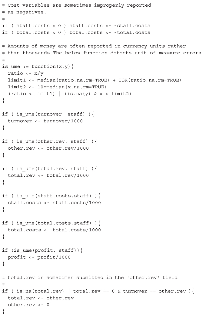
Figure 11.2 Modifying rules in modify.txt.
Besides the modifiers, we can attempt to find typographic errors in the data based on the relations forced by the validation rules. We also load the deductive package to apply correct_typos. Our script now looks like this:
  # load necesarry libraries
  library(validate)
  library(dcmodify)
  library(deductive)
  # Read data
  data(retailers, package="validate")
  # Read validation rules
  rules <- validator(.file="rules.txt")
  ## Start cleaning!
  # Read modifying rules
  mods <- modifier(.file="modify.txt")
  # apply modifiers
  retailers <- modify(retailers, mods)
  # correct typographic errors
  retailers <- correct_typos(retailers, rules)
  ## Done?
  # write data
  write.csv(retailers, file="retailers_clean.csv",row.names=FALSE)
11.1.2 Error Localization
After applying our knowledge rules and attempting to use the information in the dataset to detect typos, we are out of our wits and resort to the paradigm of Fellegi and Holt. That is, we will attempt to find for each record the least number of fields that can be altered so that all validation rules can be satisfied. We use the errorlocate package to clear these subsets of fields. For the moment, we use no weights to distinguish the reliability of variables.
  # library calls
  library(validate)
  library(dcmodify)
  library(deductive)
  library(errorlocate)
  # Read data
  data(retailers, package="validate")
  # Read validation rules
  rules <- validator(.file="rules.txt")
  ## Start cleaning!
  # Read modifying rules
  mods <- modifier(.file="modify.txt")
  # apply modifiers
  retailers <- modify(retailers, mods, sequential=TRUE)
  # correct typographic errors
  retailers <- correct_typos(retailers, rules)
  # remove sufficient fields to fix the data
  retailers <- replace_errors(retailers, rules)
  ## Done?
  # write data
  write.csv(retailers, file="retailers_clean.csv",row.names=FALSE)
11.1.3 Imputation
Our data is now at the point where observed values are deemed correct, and the missing data patterns are such that they can be imputed while satisfying every rule. Our imputation methodology will consist of two parts. First, where possible, unique imputation values will be derived based on the present values and the linear validation rules. Second, the remaining missing values will be imputed using a model-based imputation scheme. To set up model-based imputation, we first have a look at the data we have after running the error localization. Figure 11.3 displays a matrix plot of all variables occurring in the validation rules. From this overview we see that there is a reasonable linear relation between the variables, although some outliers seem still to be present. For the moment, we leave them in and use a sequence of robust methods to generate imputations. The variables total revenue and staff have the lowest missing value rates (13% and 15%), so those will be used as initial predictors. To be precise, we follow the following imputation scheme:
- 1. Use deductive imputation where possible on all variables.
- 2. Impute all variables except staff and total revenue by robust regression on predictors staff and total revenue.
- 3. Where staff is missing, regress only on total.revenue.
- 4. Use the missForest algorithm to impute the remaining missing values (in total.revenue).
We expect this will provide a reasonable first go at imputing the dataset.

Figure 11.3 The retailers data after error localization.
Using the simputation package for model-based imputation, and deductive for deductive imputation, our script now looks as follows:
  # load necesarry libraries
  library(validate)
  library(dcmodify)
  library(deductive)
  library(errorlocate)
  library(simputation)
  # Read data
  data(retailers, package="validate")
  # Read validation rules
  rules <- validator(.file="rules.txt")
  ## Start cleaning!
  # Read modifying rules
  mods <- modifier(.file="modify.txt")
  # apply modifiers
  retailers <- modify(retailers, mods, sequential=TRUE)
  # correct typographic errors
  retailers <- correct_typos(retailers, rules)
  # remove sufficient fields to fix the data
  retailers <- replace_errors(retailers, rules)
  # deductive imputation
  retailers <- impute_lr(retailers, rules)
  # impute by robust regression on staff + total.rev
  retailers <- impute_rlm(retailers
    , turnover + other.rev + staff.costs +
      total.costs + profit ∼ staff + total.rev)
  # impute by robust regression on total.rev
  retailers <- impute_rlm(retailers
    , turnover + other.rev + staff.costs +
      total.costs + profit ∼ total.rev)
  # impute using the missForest algorithm
  retailers <- impute_mf(retailers, . ∼ .)
  ## Done?
  # write data
  write.csv(retailers, file="retailers_clean.csv",row.names=FALSE)
11.1.4 Adjusting Imputed Data
All imputations were executed without taking the validation rules into account. In this final step, we will adjust imputed values using the successive projection algorithm as implemented by the rspa package. To do so, we need to record which values have been imputed so that rspa::match_restrictions knows what values to adjust. Note that the deductively imputed values need not be adjusted since these by definition are the unique solutions derived from observed data and validation rules. This gives the following completed script:
  # load necesarry libraries
  library(validate)
  library(dcmodify)
  library(deductive)
  library(errorlocate)
  library(simputation)
  library(rspa)
  # Read data
  data(retailers, package="validate")
  # Read validation rules
  rules <- validator(.file="rules.txt")
  ## Start cleaning!
  # Read modifying rules
  mods <- modifier(.file="modify.txt")
  # apply modifiers
  retailers <- modify(retailers, mods, sequential=TRUE)
  # correct typographic errors
  retailers <- correct_typos(retailers, rules)
  # remove sufficient fields to fix the data
  retailers <- replace_errors(retailers, rules)
  # deductive imputation
  retailers <- impute_lr(retailers, rules)
  # record missing values for match_restrictions
  miss <- is.na(retailers)
  # impute by robust regression on staff + total.rev
  retailers <- impute_rlm(retailers
    , turnover + other.rev + staff.costs +
      total.costs + profit ∼ staff + total.rev)
  # impute by robust regression on total.rev
  retailers <- impute_rlm(retailers
    , turnover + other.rev + staff.costs +
      total.costs + profit ∼ total.rev)
  # impute using the missForest algorithm
  retailers <- impute_mf(retailers, . ∼ .)
  # adjust imputed values to match restrictions
  retailers <- match_restrictions(retailers, rules, adjust=miss)
  ## Done!
  # write data
  write.csv(retailers, file="retailers_clean.csv",row.names=FALSE)
We can check whether the resulting data satisfies all rules after running this script. We test to an accuracy of ![]() since that is the default value used in
since that is the default value used in match_restrictions.
  library(validate)
  dat <- read.csv("R/retailers_clean.csv")
  rules <- validator(.file="R/rules.txt")
  voptions(rules, lin.eqeps=0.01, lin.ineqeps=0.01)
  confront(dat, rules)
  ## Object of class 'validation'
  ## Call:
  ##     confront(x = dat, dat = rules)
  ##
  ## Confrontations: 8
  ## With fails    : 0
  ## Warnings      : 0
  ## Errors        : 0
  sum(is.na(dat))
  ## [1] 0
So, the data is fully imputed and free of errors.
11.2 Monitoring Changes in Data
Ultimately, the data-cleaning steps used in the script rely on statistical assumptions about the data. For example, the function for detecting unit-of-measure errors assumes certain distributional properties, and the imputation models assume correlations between variables. For quality control it is helpful to have an overview of the influence that each step has on the final result. That way the risk associated with a misspecification of a modifying rule, imputation model, or localization weights can be assessed.
Schematically, we would like to extend the generic process step of the schema on page to something that looks like this:

Here, ![]() is a function that reports the difference between the input and the output of the process. Depending on the purpose of monitoring, there are several choices for
is a function that reports the difference between the input and the output of the process. Depending on the purpose of monitoring, there are several choices for ![]() . One simple way of implementing this is to create a dump of the dataset after reading and every processing step afterward. However, this type of logging consumes a lot of storage with lots of redundant information. Also, further processing is necessary afterward to interpret the results. In the following sections we discuss a few methods that summarize changes in data in more interesting ways. We also demonstrate how to do them in R. In Section 11.2.4, we return to our example data-cleaning script and show how logging changes in data can be automated over multiple processing steps with the
. One simple way of implementing this is to create a dump of the dataset after reading and every processing step afterward. However, this type of logging consumes a lot of storage with lots of redundant information. Also, further processing is necessary afterward to interpret the results. In the following sections we discuss a few methods that summarize changes in data in more interesting ways. We also demonstrate how to do them in R. In Section 11.2.4, we return to our example data-cleaning script and show how logging changes in data can be automated over multiple processing steps with the lumberjack package.
11.2.1 Data Diff (Daff)
Daff (Fitzpatrick et al., 2017) is a technical standard for expressing the difference between two tabular datasets in textual format. Its name and purpose is inspired by diff: a standard utility in the POSIX family that compares two text files. A call to diff, which is available by default on many Unix-like operating systems, may look like this:
diff <file1> <file2>The output of this call is a patch that can be used to update <file1> to <file2>. There are other uses: it can also be used to highlight differences when comparing files side by side, for instance.
The daff format describes the difference between tabular data in a way that is in itself tabular. Thus, daff patches are commonly stored as csv files. The format includes standard notation to express row insertion or deletion, column insertion, deletion, or renaming, and modified cell values.
To illustrate the syntax, we will show a few examples using the daff R package. For example,
  data(retailers, package="validate")
  library(simputation)
  library(daff)
  retailers2 <- impute_lm(retailers, turnover ∼ total.rev)
  # compute diff ('retailers' is the reference set)
  d <- diff_data(retailers, retailers2)
  # get the diff as a data.frame
  d$get_data()
  ##    @@ … staff      turnover other.rev total.rev staff.costs
  ## 1  -> …    75 NA->1113.3116        NA      1130          NA
  ## 2     …     9          1607        NA      1607         131
  ## 3 … …   …           …       …       …         …
  ## 4     …    NA          3861        13      3874         290
  ## 5  -> …    NA NA->5585.3515        37      5602         314
  ## 6     …     1            25        NA        25          NA
  ## 7  -> …     5 NA->1318.3134        NA      1335         135
  ## 8     …     3           404        13       417          NA
  ## 9 … …   …           …       …       …         …
The first row and column contain metadata. The first row denotes the column names for columns that are of importance in this diff. The first row is the action column, denoting what activity is described in the row. The first row is marked with @@ in the action column: this signals that this row contains the column names. The second row is marked with ->. This signals that a cell value has changed. Here, a missing turnover value was changed to 1113.3116. Three dots (…) signal that rows or columns have been omitted. If the action column is empty, that means that nothing changed. The extra rows and columns are there to provide enough context for the patch program to find where to apply patches.
As a second example, consider renaming a column.
  retailers3 <- dplyr::rename(retailers2, income = turnover)
  d1 <- diff_data(retailers, retailers3)
  head(d1$get_data())
  ##    ! …           +++      ---
  ## 1 @@ … vat    income turnover
  ## 2  + …  NA 1113.3116       NA
  ## 3  + …  NA      1607     1607
  ## 4  + …  NA      6886     6886
  ## 5  + …  NA      3861     3861
  ## 6  + …  NA 5585.3515       NA
We now get an extra row, marked with a !, which indicates that the set of columns (scheme) has changed. The +++ in the fourth column signals the arrival of a new column, and the --- signals the deletion of one. Note also that the values of income and turnover differ in the first row, but this is not recognized as a separate cell change. Notations of row deletions and insertions are notated along similar lines. For a full and up-to-date specification, we refer the reader to the specification website mentioned in the reference.
Using the patch_data function we can now reconstruct the changes made while going from ![]() .
.
  retailers3_reconstructed <- patch_data(retailers, d)
  all.equal(retailers3_reconstructed, retailers3)
  ## [1] "Names: 1 string mismatch"
Although the daff format is human-readable, there are some limitations to its interpretability. The patch that denotes the difference may not reflect the actual activity that took place. Indeed, the d1 patch in the above example does not reveal that changes took place in two steps. Since both the content and the name of a column have changed, an unknowing reader of the patch might conclude that a whole column was removed and a new one added (rather than imputation followed by a rename). The daff format can thus be used to accurately store all the changes made on a dataset, while the actual activities that led to those changes would need to be stored as extra information.
11.2.2 Summarizing Cell Changes
Pannekoek et al. (2014) propose a way to summarize the status of cells when comparing a dataset before and after a processing step (Figure 11.4). The idea is to count, after processing, the total number of cells in a dataset. This number is then split up into cells with available observations and missing observations. Prior to processing, these missing values either were available, which means that they were taken from the dataset (imputed), or were already missing to begin with. Similarly, the cells with values in them may have been imputed, or they were already filled prior to processing. In the latter case, the values may have changed or not.

Figure 11.4 A classification of cell status when comparing a dataset after some processing with the dataset before processing. The ‘total’ is equal to the number of cells in a dataset.
The validate package exports the cells function, which computes each of these counts for two or more datasets.
  iris1 <- iris
  iris1[1:3,1] <- NA
  iris1[2:4,2] <- iris1[2:4,2]*2
  library(validate)
  cells(start = iris, step1 = iris1)
  ## Object of class cellComparison:
  ##
  ##    cells(start = iris, step1 = iris1)
  ##
  ##                 start step1
  ## cells             750   750
  ## available         750   747
  ## missing             0     3
  ## still_available   750   747
  ## unadapted         750   744
  ## adapted             0     3
  ## imputed             0     0
  ## new_missing         0     3
  ## still_missing       0     3
cells accepts any number of data frames, comparing every data frame (except the first) with the first dataset.
  iris2 <- iris1
  iris2[1:3, 3] <- -(1:3)
  cells(start = iris, step1 = iris1, step2=iris2)
  ## Object of class cellComparison:
  ##
  ##    cells(start = iris, step1 = iris1, step2 = iris2)
  ##
  ##                 start step1 step2
  ## cells             750   750   750
  ## available         750   747   747
  ## missing             0     3     3
  ## still_available   750   747   747
  ## unadapted         750   744   741
  ## adapted             0     3     6
  ## imputed             0     0     0
  ## new_missing         0     3     3
  ## still_missing       0     3     3
It is also possible to compare data frames sequentially; for this, use the option compare="sequential".
11.2.3 Summarizing Changes in Conformance to Validation Rules
Like for cell status, one can compare the status of a dataset as measured by validation rule satisfaction after and before a data-cleaning step. Recall that when a validation rule is evaluated for a dataset, there are three possible outcomes: TRUE if the rule is satisfied, FALSE if the rule is violated, or NA if the rule cannot be evaluated because one or more of the necessary values are missing.
A classification of changes in these outcomes due to a data-cleaning step has been suggested by van den Broek et al. (2014) and is shown in Figure 11.5. In this classifications, the total number of outcomes of a validation procedure on the processed dataset is first split into outcomes that are verifiable and outcomes that are unverifiable (NA). The outcomes that are not NA can be split up further into outcomes that result in FALSE (violated) and in TRUE (satisfied). For each of those we count how many were violated (satisfied) prior to processing and how many switched from one status to the other. Similarly, we count for the currently unverifiable checks, how many were unverifiable to begin with and how many have become unverifiable.

Figure 11.5 A classification of changes in rule violation status before and after a data-cleaning step.
The validate package exports the compare function, which computes these numbers for two or more datasets. Using the same example data as in Section 11.2.2, and introducing a few rules, we get the following.
  v <- validator(
    Sepal.Length>= 0
   , Petal.Length>= 0
  )
  compare(v, start=iris, step1=iris1, step2=iris2)
  ## Object of class validatorComparison:
  ##
  ##    knitr::knit("main.Rnw", encoding = "UTF-8")
  ##
  ##                     Version
  ## Status               start step1 step2
  ##   validations          300   300   300
  ##   verifiable           300   297   297
  ##   unverifiable           0     3     3
  ##   still_unverifiable     0     0     0
  ##   new_unverifiable       0     3     3
  ##   satisfied            300   297   294
  ##   still_satisfied      300   297   294
  ##   new_satisfied          0     0     0
  ##   violated               0     0     3
  ##   still_violated         0     0     0
  ##   new_violated           0     0     3
By default, all data frames are compared to the first data frame, but they can be consecutively compared by adding the argument how="sequential".
11.2.4 Track Changes in Data Automatically with lumberjack
Tracking changes in data is fairly easy when two or more versions of a dataset are available. However, storing and handling multiple versions of a dataset quickly becomes cumbersome when multiple processing steps are involved, especially if one wishes to experiment with different steps, different parameterizations, or different orders of data-cleaning steps.
The lumberjack package offers a way to specify the logging procedure separate from the data processing. The logging action itself needs to take place between two processing steps, which is where the current dataset can be compared with the previous version. To facilitate this, the lumberjack package implements a function composition operator (also called a ‘pipe’ operator) that executes logging code when needed. The utility functions start_log(), dump_log(), and stop_log() control the logger.
Getting Started
Consider a small example, where we impute some data using simputation.
  library(validate)
  library(simputation)
  library(lumberjack)
  data(retailers)
  # we add a unique row-identifier
  retailers$id <- seq_len(nrow(retailers))
  # create a logging object.
  logger <- cellwise$new(key="id")
  out <- retailers %>>%
    start_log(logger) %>>%
    impute_lm(staff ∼ turnover) %>>%
    impute_median(staff ∼ size) %>>%
    dump_log(file="mylog.csv", stop=TRUE)
## Dumped a log at mylog.csv
Here, we first add a unique identifier to the retailers dataset since the logger we are going to use needs one. Next, a cellwise logger is created. This logger is then passed to start_logger at the beginning of the data-processing pipeline. The %>>% operator works similar to the well-known %>% operator of the magrittr1 package, except that it also makes sure that the logger gets a chance to measure the difference between the input and the output. After processing, ask the logger to dump its logging info to a csv file and to stop logging. The resulting data is stored in out.
The cellwise logger locates cells that have changed and lists a time stamp, the expression that is responsible for the change, the cell location, and its old and new values. We can inspect its output as follows:
  log <- read.csv("mylog.csv")
  head(log)
  ##   step                     time               expression key variable
  ## 1    1 2017-06-30 16:34:49 CEST impute_lm(staff ∼ turnover)  14  staff
  ## 2    1 2017-06-30 16:34:49 CEST impute_lm(staff ∼ turnover)   3  staff
  ## 3    1 2017-06-30 16:34:49 CEST impute_lm(staff ∼ turnover)  40  staff
  ## 4    1 2017-06-30 16:34:49 CEST impute_lm(staff ∼ turnover)  43  staff
  ## 5    1 2017-06-30 16:34:49 CEST impute_lm(staff ∼ turnover)   4  staff
  ## 6    2 2017-06-30 16:34:49 CEST impute_median(staff ∼ size)   5  staff
  ##   old      new
  ## 1  NA 96.88595
  ## 2  NA 10.84707
  ## 3  NA 10.61990
  ## 4  NA 10.31884
  ## 5  NA 10.56555
  ## 6  NA  1.00000
So, for example, in row 14, the variable staff was imputed by impute_lm. Such a log can give quick insights into the effect of each imputation step. For example, which function performed the most imputations?
  table(log$expression)
  ##
  ## impute_lm(staff ∼ turnover) impute_median(staff ∼ size)
  ##                           5                           1
In this case, five values were imputed in the first linear imputation step, and a single value was imputed through median imputation.
It is not necessary to put all processing steps in a single stream. The abovementioned results could also be achieved with the following code:
  # re-read data for this example
  data(retailers)
  retailers$id <- seq_len(nrow(retailers))
  logger <- cellwise$new(key="id")
  retailers <- start_log(retailers, logger)
  retailers <- retailers %>>% impute_lm(staff ∼ turnover)
  retailers <- retailers %>>% impute_median(staff ∼ size)
  dump_log(retailers,file="mylog.csv", stop=TRUE)
## Dumped a log at mylog.csv
Other Loggers
The lumberjack package is equipped with a few loggers, but it is set up in such a way that users or package authors can write their own loggers. Some loggers that are worth mentioning are the following:
- The
lbj_dafflogger that comes with thedaffpackage. It summarizes changes in cells as described in Section 11.2.1. - The
lbj_cellslogger that comes with thevalidatepackage. It summarizes changes in cells as described in Section 11.2.2. - The
lbj_ruleslogger that comes with thevalidatepackage. It summarizes changes in rule conformance as described in Section 11.2.3.
Loggers may be implemented as R Reference classes or as R6 classes, as long as they follow lumberjack's interface. This means that initializing a logger can happen in two ways. For R6 classes, it is done with <logger>$new(<options>), while for Reference classes, it is done with <logger>(<options>). In the following section, we update our example data-cleaning system and with the lbj_rules logger.
Tracking Changes in the Example
The following script is modified to use the lbj_rules logger that comes with the validate package. For compactness of presentation, all data-cleaning commands have been put into a single data pipeline. Instead of storing missing value locations for later adjustment, we store those locations by tagging the dataset using tagg_missings. This function is exported by rspa, and the tag is recognized by match_restrictions.
  library(validate)
  library(dcmodify)
  library(deductive)
  library(errorlocate)
  library(simputation)
  library(rspa)
  library(lumberjack)
  # Read data
  data(retailers, package="validate")
  # Read validation rules
  rules <- validator(.file="rules.txt")
  voptions(rules, lin.eqeps=0.01,lin.ineqeps=0.01)
  # Initialize logger.
  logger <- lbj_rules(rules)
  # tag 'retailers' for logging
  retailers <- start_log(retailers, logger)
  ## Start cleaning
  # Read modifying rules
  mods <- modifier(.file="modify.txt")
  # apply modifiers
  retailers <- retailers %>>%
    modify(mods, sequential=TRUE) %>>%
    correct_typos(rules) %>>%
    replace_errors(rules) %>>%
    impute_lr(rules) %>>%
    tag_missing() %>>%
    impute_rlm(turnover + other.rev + staff.costs +
        total.costs + profit ∼ staff + total.rev) %>>%
    impute_rlm(turnover + other.rev + staff.costs +
        total.costs + profit ∼ total.rev) %>>%
    impute_mf(. ∼ .) %>>%
    match_restrictions(rules) %>>%
    dump_log(file="cleaninglog.csv",stop=TRUE)
  ## Done!
  # write data
  write.csv(retailers, file="retailers_clean.csv", row.names=FALSE)
We can read the log as a simple csv file again and study its output.
logdata <- read.csv("R/cleaninglog.csv")The table is too large for presentation here, and so we provide a simple plot of two of its columns in Figure 11.6. We see that the number of violations first increases during the data-modifying step. This may indicate that the modifiers have too strict assumptions, for example, about the unit-of-measure errors, or perhaps not enough of them are found causing inconsistencies in balance restrictions. After the modifications, we see that the typo correction decreases the number of violations somewhat. After error localization, all violations disappear, while the number of unverifiable validations surges. This is to be expected: recall that during our error localization, step values that are deemed erroneous are removed. Next, the deductive imputation takes place, causing a drop in the unverifiables, while the number of violations stays equal to zero. This is also expected since this imputation step looks for unique values forced by the data and the validation rules. The model-based imputation steps increase the number of violations again since they do not take validation rules into account, while the number of verifiable validations steadily decreases. Finally, after adjustment, all violations disappear.

Figure 11.6 Progression of the number of violations and the number of unverifiable validations as a function of the step number in the data-cleaning process.
11.3 Integration and Automation
The example data-cleaning script contains a few parameters that may be convenient to control externally. For example, if the procedure is to be applied frequently to a new dataset, the name of the input and output files may change. Alternatively, the script may need to be integrated into a database or data analyses platform that is not R.
There are many solutions to integrate R scripts into other platforms, both commercial and open source. In this last section, we will point out a method that works on any platform since it is provided by R itself. The idea is to prepare our script for the following workflow:
- 1. A user or software creates a csv file with data to be cleaned. We cannot make any assumptions about the filename.
- 2. The file is read by the R script and processed with the steps described in Section 11.1, while a log of changes in rule failure is maintained.
- 3. After completion, a csv file with processed data and a csv file with the logging info are written to files that can be chosen by the user.
11.3.1 Using RScript
To prepare our script, one should first know that it is possible to execute an R script from the command line using the Rscript command. Here, with command line, we mean any command line supported by your operating system, for example, a bash shell for Linux or Apple users and a DOS box or Powershell for Windows users. For example, if we have a file called myfile.R
print("hello world")then the command
  $: Rscript myfile.R
  [1] "hello world"
will start R, run the script, and exit R again.
The text to print can be made configurable by passing extra arguments to Rscript and catching them with the commandArgs function. So, we change our script as follows:
  L <- commandArgs(TRUE)
  print(paste("hello ",L[[1]]))
The argument TRUE signals that the first argument (the name of the script file) is of no importance to us. The result of a call to commandArgs is a list. Here is how to use it ($ denotes the command prompt).
  $ Rscript myscript.R "happy user"
  [1] "hello  happy user"
11.3.2 The docopt Package
As scripts become more involved, and the number of options grows, parsing all options retrieved with commandArgs can become cumbersome. The docopt package makes defining and processing options much easier while also automatically creating a help index for the script. Below is our little running example, but now using docopt.
  suppressPackageStartupMessages(library(docopt))
  "
  Usage: myscript.R [-h STRING]
  -h      Show this help
  STRING  The string to print after 'hello'
  " -> doc
  opt <- docopt(doc)
  print(paste("hello ",opt$STRING))
In the first line we quietly load the package. Next, we create a string literal, stored in doc that is precisely the help information to be printed when a user requires it. The first line of the help info specifies how the command can be called: either with -h or with a string (the ‘or’ is implied by putting both arguments between square brackets). The help info also specifies that --help works as well. By calling opt <- docopt(doc) the command-line arguments are parsed and stored in opt. The latter object is a named list.
  $ Rscript myscript.R -help
  Usage: myscript.R [-h STRING]
  -h      Show this help
  STRING  The string to print after 'hello'
  $ Rscript myscript.R "pretty User"
  [1] "hello  pretty User"
11.3.3 Automated Data Cleaning
In Figure 11.7, the adapted data-cleaning script is shown. The input file, output file, validation rule file, and modifying rule file have all been made changeable optionals. The docopt package is used for argument handling and will provide an informative message if an option is missing, for example. Further automation steps could make the script more robust, for example, by checking whether files exist, making modifying rules optional, and so on. Whether this is desirable is up to the agreement between the provider and the user of the script and therefore is beyond the scope of this book.

Figure 11.7 The completed data-cleaning script, automated using docopt.