Chapter 6
Data Validation
6.1 Introduction
Data validation—confirming whether data satisfies certain assumptions from domain knowledge—is an essential part of any statistical production process. In fact, a recent survey among the 28 national statistical institutes of the European Union shows that an estimated 10–30% of the total workload for producing a statistic concerns data validation (ESS, 2015). Even though these numbers can be considered only as rough estimates, their order of magnitude clearly indicates that it is a substantial part of the workload. For this reason, the topic of data validation deserves separate attention.
The demands that a dataset must satisfy before it is considered fit for analyses can usually be expressed as a set of short statements or rules rooted in domain knowledge. Typically, an analyst will formulate a number of such assumptions and check them prior to estimation. Some practical examples taken from the survey mentioned earlier (rephrased by us) are as follows:
- If a respondent declares to have income from ‘other activities’; fields under ‘other activities’ must be filled.
- Yield per area (for a certain crop) must be between 40 and 60 metric tons/ha.
- A person below the age of 15 cannot take part in economic activity.
- The field ‘type of ownership’ (for buildings) may not be empty.
- The submitted ‘regional code’ must occur in the official code list.
- The sum of reported profits and costs must add up to the total revenue.
- The persons in a married couple must have the same year of marriage.
- If a person is a child of a reference person, then the code of the person's father must be the reference person's code.
- The number of employees must be equal to or greater than zero.
- Date of birth must be larger than December 30, 2012 (for a farm animal).
- Married persons must be at least 15 years old.
- If the number of employees is positive, the amount of salary paid must be positive.
- The current average price divided by last period's average price must lie between 0.9 and 1.1.
The examples include rules where values are compared with constants, past values, values of other variables, (complex) aggregates, and even values coming from different domains or datasets.
The set of knowledge-based validation rules for a dataset can thus be varied and, depending on the number of variables and known relationships between them, may be large. Moreover, since any single variable may occur in several rules, validation rules are often interconnected and may therefore give rise to redundancies or contradictions. For this reason, a systematic way of defining rules, confronting data with them, and maintaining and analyzing rule sets is desirable. From a theoretical point of view, this means that we need a solid (mathematical) definition of what data validation rules are, investigate their properties, and find out in what ways they may be manipulated. From a practical perspective, it means that we need a system where rules can be defined and manipulated independent of the data. Such a system has the added benefits of being able to reuse rule sets across (similar) datasets and allowing for unambiguous communication of rules between different parties working with the data or statements based on them.
To get a feel of what such system can do, we start this chapter by treating a few practical examples using the validate package (van der Loo and de Jonge, 2015b). Next, we dive in a little deeper and discuss a formal definition of data validation and give some general properties of sets of data validation rules, followed by a more extensive discussion of validate.
6.2 A First Look at the validate Package
The validate package implements a set of objects and methods that together form an infrastructure for data validation. The main purpose of validate is to provide a solid basis for rule declaration (separate from data) either from the command line or file, managing rule metadata, confrontating data with the rules and gathering the results, and summarizing and analyzing such results in a meaningful way.
In this chapter we will demonstrate functionality validate using the retailers dataset that comes with the package. This raw data file consists of 60 records of anonymized economic information on retailers (supermarkets), with many commonly occurring errors and missing values. Variables include the number of staff, the amount of turnover and other revenues, the total revenue, staff costs, total costs, and the amount of profit in thousands of guilders. The data can be loaded as follows:
  library(validate)
  data(retailers)
A complete description of the dataset can be found in the help file by typing ?retailers at the command line.
6.2.1 Quick Checks with check_that
The simplest way to perform validation tasks is to use the check_that function. It accepts a data.frame and one or more rules. In the following example we check the following assumptions:
- Turnover is larger than or equal to zero.
- The costs per staff are below fl
 .
.
Using check_that, this is done as follows:
cf <- check_that(retailers, turnover > 0, staff.costs/staff < 50)The object cf, storing the validation results, is an object of class confrontation, and it stores all the results of confronting the data in retailers with the validation rules. Using summary, we get an overview per rule.
  summary(cf)
  ##   rule items passes fails nNA error warning             expression
  ## 1   V1    60     56     0   4 FALSE   FALSE           turnover > 0
  ## 2   V2    60     39     5  16 FALSE   FALSE staff.costs/staff < 50
This tells us the following: 60 records were tested against each rule. The first rule, testing positivity of the turnover variable, was satisfied by 56 records. It was failed by none, but in four cases it yielded NA. Evaluating the rule did not result in errors or warnings. The second rule, a sanity check on costs per staff, was satisfied by 39 records, failed by 5, and could not be computed because of missing values in 16 cases. Furthermore, the last column shows the R expression that was evaluated to compute the outcome of each rule, and the sixth and seventh columns indicate whether an evaluation resulted in a warning or an error. The first column shows the name of the rules which in this case was assigned automatically.
Observe that in the above statement the rules have been defined without a reference to the data. We could use almost the same function call, changing only the dataset to another dataset also containing the variables turnover, staff.costs, and staff. This separation of rules and data is critical for performing data validation in a systematic way.
The rules that can be handled by validate may be arbitrarily complex as long as they are actual validation rules (more on that later). As a demonstration we add two rules to the running example. The first rule states that the average profit should be positive, reflecting our intuition that even though individual profits may be negative, the sector as a whole is profitable. The second rule states our expectation that if a retailer has staff, its staff costs should exceed zero.
Introducing the above rules in the running examples yields the following check:
  cf <-  check_that(retailers
      , to = turnover > 0
      , sc = staff.costs/staff < 50
      , cd = if ( staff > 0 ) staff.costs > 0
      , mn = mean(profit,na.rm=TRUE) > 0
    )
Here, we also gave our rules a short name (for printing purposes) that is copied in the summary.
  summary(cf)
  ##   rule items passes fails nNA error warning        expression
  ## 1   to    60     56     0   4 FALSE   FALSE      turnover > 0
  ## 2   sc    60     39     5  16 FALSE   FALSE      staff.costs/
staff < 50
  ## 3   cd    60     50     0  10 FALSE   FALSE    !(staff > 0) |
 staff.costs > 0
  ## 4   mn     1      1     0   0 FALSE   FALSE      mean(profit,
 na.rm = TRUE) > 0
Observe that for the rule we named ‘mn’, only one item was checked. The rule applies to the whole turnover column and not to individual values. Furthermore, observe that the expression for the conditional rule printed in the summary is different from the one we used as input. The input rule if (staff > 0) staff.costs > 0 is translated to the equivalent !(staff>0)|staff.costs > 0 by validate for faster (vectorized) execution. The summary function will always show the expression as it was used during evaluation.
We can create a bar plot for the multi-item rules by selecting the first three results and passing them to barplot.
barplot(cf[1:3],main="Retailers")
This horizontally stacked bar chart represents the number of items (records) failing, passing, or resulting in missing values for each rule. In fact, we could have plotted the whole cf object not just the results of the first three rules. We leave as an exercise for the reader to try this out and see how barplot handles validation outputs with different dimension structures.
6.2.2 The Basic Workflow: validator and confront
The above examples are nice for quick checks on data on the command line or in simple scripts. For more systematic data validation and rule manipulation, it is better to separate the definition, storage, and retrieval of rules from other activities.
Validation rules can be stored in a validator object. The function validator reads rules from the command line or from file.
  v <- validator(
      turnover > 0
    , staff.costs / staff < 50
    , total.costs >= 0
    , staff >= 0
    , turnover + other.rev == total.rev
  )
  v
  ## Object of class 'validator' with 5 elements:
  ##  V1: turnover > 0
  ##  V2: staff.costs/staff < 50
  ##  V3: total.costs >= 0
  ##  V4: staff >= 0
  ##  V5: turnover + other.rev == total.rev
Data can be confronted with these rules using confront (not check_that).
  cf <- confront(retailers, v)
  cf
  ## Object of class 'validation'
  ## Call:
  ##     confront(x = retailers, dat = v)
  ##
  ## Confrontations: 5
  ## With fails    : 2
  ## Warnings      : 0
  ## Errors        : 0
The result is a confrontation object that stores all information relevant to the validation just performed. When printed to the screen, it shows the call that generated it, how many rules have been executed, how many of them were failed at least once, how many of them resulted in errors, and how many raised a warning.
We have seen in the previous section how results stored in a confrontation object can be analyzed using summary or barplot. More detailed output can be obtained with the values function (we use head to limit the printed output).
  head(values(cf))
  ##        V1   V2   V3   V4    V5
  ## [1,]   NA   NA TRUE TRUE    NA
  ## [2,] TRUE TRUE TRUE TRUE    NA
  ## [3,] TRUE   NA TRUE   NA FALSE
  ## [4,] TRUE   NA TRUE   NA  TRUE
  ## [5,]   NA   NA TRUE   NA    NA
  ## [6,] TRUE   NA TRUE TRUE    NA
The values are returned in an array of class logical, where each column represents a rule, and each row represents a record. The value TRUE means that a rule is satisfied by the validated item, and the value FALSE means that the rule is violated. A missing value (NA) indicates that a rule is evaluated to missing. For example, from the above output, we read that in the third record, V1 (turnover positivity) is satisfied, V5 (a balance check) is violated, and V2 (a bound on the costs per staff member) could not be evaluated. We may inspect the record to spot the cause of this.
  retailers[3,c("staff","staff.costs")]
  ##   staff staff.costs
  ## 3    NA         324
In this case, the variable staff is missing.
Summarizing, the basic work flow for data validation suggested by the validate package is as follows:
- 1. Define a set of rules; using
validator. - 2. Confront data with the rules using
confront. - 3. Analyze the results, either with built-in functions or with your own methods after extracting the results.
The check_that function is just a simple wrapper that combines the first two steps.
In Section 6.5, we elaborate further on these steps, including how to store and retrieve rules from text files and several ways to analyze the results.
6.2.3 A Little Background on validate and DSLs
The validate package implements a domain-specific language (DSL) for the purpose of data validation. Fowler (2010) defines a DSL as
a computer programming language of limited expressiveness focused on a particular domain.
Indeed, many DSLs lack a lot of the properties one expects from a ‘proper’ programming language such as abstractions for recursion, iteration, or branching. Nevertheless, many DSLs are considered highly successful. Examples include regular expressions and generalizations thereof and markup languages such as markdown, html, or yaml.
Over time, a number of DSLs have been implemented in R (and previously S), both in the R core distributions as well as in packages. Examples include base R's formula–data interface for the specification of statistical models, the R implementation of the grammar of graphics (Wickham, 2009; Wilkinson, 2005), and the editrules package for in-record validation and error localization (de Jonge and van der Loo, 2015), the predecessor of validate.
The above examples demonstrate that there are two kinds of DSLs: those defined on its own that allow for different implementations and those defined as a subset or reinterpretation of an existing language. Gibbons (2013) refers to the latter category as embedded and to the former as standalone DSLs. Clearly, validate's DSL is embedded in R, since the validating statements are formulated in R syntax and reinterpreted by the package to produce validation outcomes. The fact that R hosts a number of DSLs comes as no surprise since, according to the same author ‘it turns out that functional programming languages are particularly well suited for hosting embedded DSLs’.
There are many advantages to implementing a data validation syntax embedded into R. First, R's facilities to compute on the language including access to the abstract syntax tree of statements and nonstandard evaluation make experimenting with such an implementation a breeze. In particular, it makes it easy to experiment with different ideas and test them out in practice, something which is much harder while developing a standalone DSL. Second, using R as a host language means access to the truly enormous data processing and statistical capabilities that come with R and its packages at no cost whatsoever. Third, many users interested in data validation are already familiar with R and will be able to use the DSL with relative ease.
The downside of embedding a DSL into another language includes leakage: a user may (unwittingly) ‘escape’ the DSL and use more advanced features of the host language. A second downside is that the syntax of the host language may be too limited to accurately capture the concepts for which the DSL was designed. It is of interest to note that R is more flexible than many other languages, since it allows for the definition of user-defined infix operators. The most famous example is probably the pipe operator %>% of the magrittr package.
To accommodate for the possible leakage problem, the validate package filters out statements that are not ‘validating statements’ when defining a validator. For example, trying to include a rule that does not ‘validate’ anything results in a warning.
v <- validator( x > 0, mean(y))To be able to decide what statements actually form a validating rule and to decide what are the relevant (algebraic) operations on sets of such rules, we are going to need a more formal definition of data validation.
Exercises for Section 6.2
6.3 Defining Data Validation
At the core, data validation is a falsification process. That is, one tries as much as possible to make assumptions about data explicit and verifies whether they hold up in practice. Once sufficient assumptions have been tried and tested, one considers a dataset fit for use, that is, valid. Not performing any validation corresponds to blindly assuming that the values recorded in a dataset are acceptable as a facts, in the sense that they are usable for the production of statistical statements.
Every assumption made explicit through a data validation process limits the set of acceptable values or value combinations. In words, data validation can therefore be defined as follows (ESS, 2015; van der Loo, 2015b):
Data validation is an activity that consists of verifying whether a collection of values comes from a set of predefined collections of values.
As we saw in the earlier examples, the term ‘collection of values’ may consist of a single value only (as in: turnover must be nonnegative). Also, the term ‘predefined’ should be interpreted generally. In many cases, the set of ‘acceptable values’ or combinations thereof is not defined explicitly but rather as a set that is implied by an involved calculation. As an example, consider the rule where we deem a numerical record invalid when it is more than some distance ![]() removed from the mean vector of the data, where the distance is computed as the Mahalanobis distance. In this case, the calculation involves estimating the (inverse) covariance matrix, computing the distance with the mean vector, and comparing the result with
removed from the mean vector of the data, where the distance is computed as the Mahalanobis distance. In this case, the calculation involves estimating the (inverse) covariance matrix, computing the distance with the mean vector, and comparing the result with ![]() . The set of allowed or disallowed records is not defined explicitly. However, since the procedure of validation is fully deterministic (and we assume this to be the case in all validation procedures), we deem the collection of valid value combinations predetermined.
. The set of allowed or disallowed records is not defined explicitly. However, since the procedure of validation is fully deterministic (and we assume this to be the case in all validation procedures), we deem the collection of valid value combinations predetermined.
The above definition includes validation activities made explicit through (mathematical) validation rules as well as procedural validation such as expert review based on fixed methodology. In this work, we limit ourselves to data validation procedures that can be fully automated, which is why we move on to discuss a formal definition that underlies choices made in the validate package.
6.3.1 Formal Definition of Data Validation
Since validation is a process that consists of decision-making about data, it is tempting to define a validation function mathematically as a function that takes a collection of data and returns 0 (invalid) or 1 (valid). There are, however, some subtleties to take care of when constructing such a definition. Most importantly, we need to construct precisely what the domain of such a function is. Considering the examples in Section 6.2, the domain must encompass single values, records, columns, multiple tables, or any other collection of data points. Simply stating that the domain is ‘the set of all datasets’ will not do, because this is not a proper set-theoretical definition: the set of all datasets contains itself recursively.
To solve this, we first define a data point as follows:
The purpose of the key is to make the corresponding value identifiable in a collection of data. At the very least it identifies the variable of which the value is a realization, but a key is often represented by a collection of subkeys that together identify the statistical unit, the variable, the measurement, and so on. For the moment the precise information stored in the key is unimportant, but in Section 6.4 we will discuss a general set of keys that allow us to classify data validation functions. The value domain, ![]() , depends on the context in which the value is obtained. It is the basic domain on top of which further assumptions must be checked. For example, if we know all values are integers, the domain
, depends on the context in which the value is obtained. It is the basic domain on top of which further assumptions must be checked. For example, if we know all values are integers, the domain ![]() is
is ![]() , and if no type-checking took place, one can set the domain to the set of strings
, and if no type-checking took place, one can set the domain to the set of strings ![]() over a suitable alphabet
over a suitable alphabet ![]() . If the value can be either text or integer, the domain can be defined as
. If the value can be either text or integer, the domain can be defined as ![]() .
.
Given a set of keys ![]() and a domain
and a domain ![]() , the set of all possible key-value pairs is the Cartesian product
, the set of all possible key-value pairs is the Cartesian product ![]() . A dataset can now be defined as follows:
. A dataset can now be defined as follows:
An informal way of stating this definition is to say that a unique measurement must yield a unique value. A more technical way of stating this is to say that a dataset is a function from ![]() to
to ![]() . We denote the set of all datasets associated with
. We denote the set of all datasets associated with ![]() and
and ![]() as
as ![]() .
.
The above example shows that our formulation of a dataset is very tolerant in the sense that it allows to store a logical value for a numerical variable and vice versa. As a consequence, our definition of validation will include type-checking.
So a formal data validation function accepts a complete dataset in ![]() and returns 0 (invalid or ‘false’) or 1 (valid or ‘true’). Validation functions are defined to be surjective (onto) since functions that by their definition always return 1 are not informative (all data satisfies the assumption expressed by the function), and functions that always return 0 are contradictions: no collection of data in
and returns 0 (invalid or ‘false’) or 1 (valid or ‘true’). Validation functions are defined to be surjective (onto) since functions that by their definition always return 1 are not informative (all data satisfies the assumption expressed by the function), and functions that always return 0 are contradictions: no collection of data in ![]() can satisfy the assumption expressed by the function. Surjectivity is thus implied by the notion that validation is really an attempt to falsify assumptions we might have about the properties of a dataset. Any test that by definition is always failed or always passed cannot be an attempt at falsification.
can satisfy the assumption expressed by the function. Surjectivity is thus implied by the notion that validation is really an attempt to falsify assumptions we might have about the properties of a dataset. Any test that by definition is always failed or always passed cannot be an attempt at falsification.
Any validation function ![]() by definition separates
by definition separates ![]() into two regions. The valid region is defined as the preimage
into two regions. The valid region is defined as the preimage ![]() . The corresponding invalid region is defined as
. The corresponding invalid region is defined as ![]() . Given a set of validation functions, the valid region is the intersection of their respective valid regions. Since it is in general not guaranteed that the intersection of two or more valid regions is nonempty, care must be taken when formulating such sets. We will return to this in the following section, but let us first conclude with some remarks on practical issues.
. Given a set of validation functions, the valid region is the intersection of their respective valid regions. Since it is in general not guaranteed that the intersection of two or more valid regions is nonempty, care must be taken when formulating such sets. We will return to this in the following section, but let us first conclude with some remarks on practical issues.
The example validation functions in Section 6.3.5 are defined in a formal way which is not how one usually defines or discusses them. For example, instead of writing a function that checks the relation between job status and age for each individual record, one formulates the rule
and simply implies that it must hold for each record separately.
6.3.2 Operations on Validation Functions
For effective reasoning about validation functions, it is important to consider the basic operations under which the set of validation functions on a certain domain ![]() is closed. Since the result of a validation function is boolean, it is tempting to try to combine validation functions with the standard boolean operators, negation (
is closed. Since the result of a validation function is boolean, it is tempting to try to combine validation functions with the standard boolean operators, negation (![]() ), conjugation (
), conjugation (![]() ), and disjunction (
), and disjunction (![]() ) by defining
) by defining ![]() ,
, ![]() , and
, and ![]() .
.
For the ![]() operation, we have the following observation, which is proven in Exercise 6.3.2.
operation, we have the following observation, which is proven in Exercise 6.3.2.
It follows that combining validation functions by disjunction does not necessarily result in another validation function since the property of surjectivity may be lost. That is, one can think of cases where the outcome of ![]() equals 1 for every dataset in
equals 1 for every dataset in ![]() .
.
The most important practical consequence of the above result is that one needs to be careful when defining validation rules consisting of several disjunctions. Especially for validation functions that involve complex calculations or derivations, determining the valid region explicitly may be hard.
The following observation also has practical consequences since it limits what validation functions can be put together in a set.
It follows from this observation that two validation functions cannot in general be conjuncted to form another validation function. In particular, this happens when ![]() and
and ![]() contradict.
contradict.
A practical consequence of the above result is that when one defines multiple validation functions on a dataset, which amounts to joining them by conjunction, one needs to check if no contradictions occur. In principle, given a set of validation functions ![]() , one can confirm that it is internally consistent by computing the preimage
, one can confirm that it is internally consistent by computing the preimage
It is easy to see that ![]() if and only if for some
if and only if for some ![]() , we have
, we have ![]() . In reality, however, computing the valid region explicitly can be a daunting if not an impossible task. In practice, algorithms for confirming or rejecting the internal consistency for a set of rules exist only for some classes of validation functions such as linear (in)equalities and certain logical assertions.
. In reality, however, computing the valid region explicitly can be a daunting if not an impossible task. In practice, algorithms for confirming or rejecting the internal consistency for a set of rules exist only for some classes of validation functions such as linear (in)equalities and certain logical assertions.
Let us briefly summarize what we have found so far. After stating that validation is an attempt to falsify assumptions about a dataset, we found that this notion could be formalized as a surjective function that has as codomain the boolean set ![]() . This surjectivity then, places strong restrictions on how we may combine such functions to form new ones. Essentially, we can only guarantee with certainty that the negation of a validation function is also ‘validating’, but with opposite results, and we have to be careful when defining sets of validation functions.
. This surjectivity then, places strong restrictions on how we may combine such functions to form new ones. Essentially, we can only guarantee with certainty that the negation of a validation function is also ‘validating’, but with opposite results, and we have to be careful when defining sets of validation functions.
6.3.3 Validation and Missing Values
In the previous discussion we have quietly assumed that validation functions can always be computed, and in the strict sense this is true. If one allows the missingness indicator NA in the measurement domain ![]() , one can always define validation functions such that NA is handled as a specific case. For example, consider a single numerical variable
, one can always define validation functions such that NA is handled as a specific case. For example, consider a single numerical variable ![]() with the measurement domain
with the measurement domain ![]() , so
, so ![]() might be missing after measurement. Suppose that we have the rule that
might be missing after measurement. Suppose that we have the rule that ![]() must be positive. We could define the validation function as follows:
must be positive. We could define the validation function as follows:

Here, the result is explicitly set to 0 if ![]() is missing. Such definitions quickly become cumbersome when
is missing. Such definitions quickly become cumbersome when ![]() involves multiple variables, since the check for missingness has to be included explicitly for every variable. It is therefore desirable to choose a default value for such cases.
involves multiple variables, since the check for missingness has to be included explicitly for every variable. It is therefore desirable to choose a default value for such cases.
Two obvious choices present themselves: either every calculation that cannot be completed because of a missing value results in 0, and the definition of validation functions remains the same, or missingness is propagated through the calculation, and the codomain of validation functions is extended from ![]() to
to ![]() . There is a third option that maps every missing value to 1 (valid), but this does not seem to have a meaningful interpretation.
. There is a third option that maps every missing value to 1 (valid), but this does not seem to have a meaningful interpretation.
The advantage of extending the codomain to ![]() is that one obtains a more detailed picture from the validation results. The disadvantage is that analyses of validation results become slightly more complex. In the R package
is that one obtains a more detailed picture from the validation results. The disadvantage is that analyses of validation results become slightly more complex. In the R package validate, propagation of missingness is the default (as it is in R) but this behavior can be controlled by the user.
6.3.4 Structure of Validation Functions
As shown in the examples of Sections 6.1 and 6.2, validation functions may involve arbitrarily complex calculations. The result of such a calculation is then compared with a range of valid calculation results. As an example, reconsider the following rule, mentioned in the introduction:
The current average price divided by last period's average price must lie between 0.9 and 1.1.
This rule can be stated as (![]() denoting price).
denoting price).

where ![]() denotes the range
denotes the range ![]() . To evaluate this rule, first the average prices at time
. To evaluate this rule, first the average prices at time ![]() and
and ![]() are determined, and next, the result is compared with the range
are determined, and next, the result is compared with the range ![]() . As another example, consider the rule
. As another example, consider the rule
the sum of cost and profit must equal revenue.
This can be written as (denoting ![]() for cost,
for cost, ![]() for profit, and
for profit, and ![]() for revenue)
for revenue)
We first compute the linear combination on the left-hand side and then check set membership with the valid computed value set ![]() . Finally, consider the rule
. Finally, consider the rule
if the number of staff is larger than zero, the amount of salary paid must be larger than zero.
Using the implication replacement rule, we may write
Again, we need to perform a calculation on the left-hand side and compare the result with a valid computed set (![]() ) in this case.
) in this case.
This above suggest that it may be useful write a validation function ![]() as a compound function (van der Loo and Pannekoek, 2014)
as a compound function (van der Loo and Pannekoek, 2014)
that is, ![]() . Here,
. Here, ![]() is often referred to as a score function that computes an indicator, usually a single number or other (categorical) values from the input dataset
is often referred to as a score function that computes an indicator, usually a single number or other (categorical) values from the input dataset ![]() . The function
. The function ![]() is the set indicator function, returning 1 if its argument is in
is the set indicator function, returning 1 if its argument is in ![]() and 0 otherwise. In practice, it may occur that
and 0 otherwise. In practice, it may occur that ![]() cannot be computed because of missing values. In such cases, we define that the result is
cannot be computed because of missing values. In such cases, we define that the result is ![]() and
and ![]() as well.
as well.
To see what this all means, let us work through the above examples. In the example of Eq. (6.2), we have

where ![]() and
and ![]() are vectors of observed values and
are vectors of observed values and ![]() their estimated means. In example (6.3.4), we have
their estimated means. In example (6.3.4), we have
For the final example, we may define ![]() and
and ![]() as follows:
as follows:

Using the decomposition of Eq. (6.3), we see that a validation function can be fully defined by specifying a score function ![]() and a region
and a region ![]() of valid scores. An interesting special case occurs when we choose
of valid scores. An interesting special case occurs when we choose ![]() to be the identity function:
to be the identity function: ![]() . In that case
. In that case ![]() is equal to the valid region in
is equal to the valid region in ![]() :
: ![]() . Simple range checks fall in this category. For example, the rule
. Simple range checks fall in this category. For example, the rule ![]() can be written as
can be written as ![]() .
.
6.3.5 Demarcating Validation Rules in validate
When constructing a set of validation rules with the validator function, the parser of validate must decide whether the statements the user specifies are actually validating rules (functions) as in Definition 6.3.4. This definition comprises two aspects that are checked by the constructor: validation rules must yield a value in ![]() , and validation rules must be surjective.
, and validation rules must be surjective.
The latter condition is checked by verifying that the expressions submitted by the user contain at least one variable, so the result can in principle vary when confronted with different values for that variable. This means that statements like
1 > 0are filtered from the input (with a warning).
To test whether the first condition is satisfied, that is, whether the rule expresses a validating function, we need to check the following options. The final operation when evaluating a validation function is either
- a set membership function (i.e.,
%in%,<,==, some specialized R functions), - a logical quantification or existence operator (
all,any, some specialized R functions) or - the negation of such an expression.
Due to R's flexibility, there are in principle two loopholes that may cause this check to fail. Users may locally overwrite standard functions such as "<" with an arbitrary two-parameter function. To cope with this situation, the constructor checks whether this has happened and emits a warning if it is the case. Alternatively, users may define a constant score function, thereby hiding the nonsurjectivity of the rule from this analysis. For example, the rule
x - x == 0will always yield true and is accepted by validate. Although it is impossible to rule out all such cases, in Chapter 8, we shall see how for certain classes of rule sets contradictions and redundancies can be flushed out automatically.
The above operations are a translation of the strict definition of validation functions (6.3.4) and the allowed operations on them. As a compromise to usability, the strictly allowed expressions may still be combined using boolean operators (and, or, exclusive or, implication) and quantifiers (for all, exists) in validate. As discussed before, it can not be guaranteed that boolean combinations of validation functions are also validation functions in the strict sense of Definition 6.3.4. It is therefore up to the user to make sure that no rules that are constant by definition are submitted.
The allowed syntax can be symbolically summarized with the following syntax diagram:

Here, boolean expression is an R expression that is confirmed to result in a logical and contain at least one variable. Note that this diagram allows for implication (![]() ) since
) since ![]() and exclusive or (
and exclusive or (![]() ) since
) since ![]() . There are several ‘syntactic sugar’ options to support such statements. For example
. There are several ‘syntactic sugar’ options to support such statements. For example if and xor are allowed specifically. A more complete description of the options is given in Section 6.5.
Exercises for Section 6.3
6.4 A Formal Typology of Data Validation Functions
In the previous sections we saw several kinds of validation rules such as in-record and cross-record rules, cross-dataset rules, and so on. On one hand, this subdivision in rule types is more or less intuitive as it is closely related to everyday thinking about data in terms of fields, records, and tables. On the other hand, it is not a very robust subdivision. For example, merging two files can turn a cross-dataset validation rule into an in-dataset validation rule.
Having a more robust typology has benefits. It allows one to compare validation processes over different statistical production processes or to compare the capabilities of various softwares implementing validation methods. In the following sections we discuss a method for classifying data validation functions by studying the type of sets of data points they take as input. For this, we need to have a minimal set of keys that identify a value, which is the topic of the following section. The discussion in this section is largely based on a paper by van der Loo (2015b), which in itself was inspired partly by a paper of Gelsema (2012),
6.4.1 A Closer Look at Measurement
Recall that we defined a data point as the combination of a set of keys and a single value. The purpose of the key set is to identify the value: what variable is it, the property of which statistical object it measures, and so on. In this section, we discuss a minimum set of keys that describe a data point obtained by a statistical measurement. In the following section, these keys will be used to classify validation rules.
To find a set of keys that identify a value, let us have a closer look at how a data point is obtained by measurement. Figure 6.1 gives an overview of the timeline involved in creating a data point. At some time, ![]() a statistical object is born or created. This may be a person, a company, a phone call, an e-mail, or any other event or object of interest. In any case, we can think of
a statistical object is born or created. This may be a person, a company, a phone call, an e-mail, or any other event or object of interest. In any case, we can think of ![]() as an element of a set
as an element of a set ![]() of objects of equal type, where
of objects of equal type, where ![]() contains all objects that ever lived, live now, and ever will live. From
contains all objects that ever lived, live now, and ever will live. From ![]() onward, the object of interest has some properties, say
onward, the object of interest has some properties, say ![]() , that may or may not vary over time. At time
, that may or may not vary over time. At time ![]() , we choose to select
, we choose to select ![]() for measurement and to measure the value of
for measurement and to measure the value of ![]() . The actual measurement may pertain to the value of
. The actual measurement may pertain to the value of ![]() at time
at time ![]() , or it may pertain to an earlier time (e.g., we may ask a person, did you have a job last year?) or even a time in the future (do you expect to have a job next year?). For the current discussion these times are immaterial: we are only interested in the time of measurement
, or it may pertain to an earlier time (e.g., we may ask a person, did you have a job last year?) or even a time in the future (do you expect to have a job next year?). For the current discussion these times are immaterial: we are only interested in the time of measurement ![]() since that determines on which population the final statistical statement will be based. The time to which a measurement pertains is interpreted as belonging to the definition of the measured variable
since that determines on which population the final statistical statement will be based. The time to which a measurement pertains is interpreted as belonging to the definition of the measured variable ![]() . Finally, sometime after the measurement took place, the element
. Finally, sometime after the measurement took place, the element ![]() disappears from the current population at
disappears from the current population at ![]() .
.
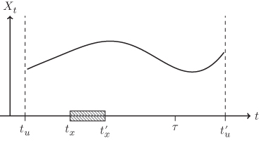
Figure 6.1 The various times involved in a measurement process. A population member  exists over the period
  . At the time of measurement
  , a value of
  is observed pertaining to the period
  . In principle,
  may be before, within, or after this period. Also, instead of a period, one may choose a moment in time by letting
  .
.
Based on this discussion, we find four aspects that identify a data point. These are as follows:
- The set
 that represents all objects of a certain type that ever were, are, and will be;
 - The time of measurement
 , which determines what part of
  is active;
 - The element
 , chosen at time
  ;
; - The variable
 that is measured.
If we denote the timeline with ![]() and the domain of
and the domain of ![]() with
with ![]() , a measurement can be represented as a series of maps
, a measurement can be represented as a series of maps
where ![]() is the population at time
is the population at time ![]() ,
, ![]() selects element
selects element ![]() from
from ![]() , and
, and ![]() results in a value in
results in a value in ![]() .
.
As an example, let us see what the values for these keys are for the retailers dataset in the validate package. The set ![]() consists of all Dutch retailers ever, past, present, and future. Now that is a big set, and it is impossible to construct explicitly, but since it only serves to indicate with what objects we are dealing that is fine. The time of measurement
consists of all Dutch retailers ever, past, present, and future. Now that is a big set, and it is impossible to construct explicitly, but since it only serves to indicate with what objects we are dealing that is fine. The time of measurement ![]() is the time at which the survey was executed (including establishing the survey frame). In practice, this time is hard to establish already because survey execution will take a time span rather than a moment in time. That is no problem for this model:
is the time at which the survey was executed (including establishing the survey frame). In practice, this time is hard to establish already because survey execution will take a time span rather than a moment in time. That is no problem for this model: ![]() may be implemented as a unique identifier for the survey as long as it uniquely identifies the current population from which the survey was drawn. The element
may be implemented as a unique identifier for the survey as long as it uniquely identifies the current population from which the survey was drawn. The element ![]() corresponds to a single interviewed retailer and therefore with one record in the actual data. The measured variable is any of the columns obtained in the survey, for example staff costs (and it pertains to the period preceding the period of measurement).
corresponds to a single interviewed retailer and therefore with one record in the actual data. The measured variable is any of the columns obtained in the survey, for example staff costs (and it pertains to the period preceding the period of measurement).
To check the validity of values in the retailers dataset, one may perform cell-by-cell checks, check the variable averages against each other, or compare aggregates of variables with aggregates of a dataset pertaining to a different population (wholesalers, say). Depending on the validation rule, different slices of a dataset are needed, or to put it otherwise, different keys need to be varied over in order to be able to compute the validation function. This is the idea behind the following classification.
6.4.2 Classification of Validation Rules
The idea behind the classification discussed here is that we label each basic key in ![]() whether its value must be varied over in order to compute a particular validation function. Naively, we obtain
whether its value must be varied over in order to compute a particular validation function. Naively, we obtain ![]() categories, labeled according to whether one must vary no keys (1 option), a single key (4 options), two keys (6 options), three keys (4 options), or four keys (1 option). However, this number is diminished since the keys cannot be varied completely independent of each other.
categories, labeled according to whether one must vary no keys (1 option), a single key (4 options), two keys (6 options), three keys (4 options), or four keys (1 option). However, this number is diminished since the keys cannot be varied completely independent of each other.
First, once the domain is chosen, the type of statistical objects is fixed, which implies that the chosen properties (variables) are fixed as well. As a consequence, validation rules that pertain to different domains must also pertain to different variables. Confusingly, variables for different object types often have similar names. For example, the variable name income may relate to a household, a person, or a company. Indeed, these are all some types of incomes, but since they relate to a different object type and are measured in a different way, they must be considered as separate variables nonetheless. For this reason, validation rules that pertain to a multiple domains must also pertain to different variables.
Second, observe that even though an object can be represented in multiple domains (e.g., companies and companies with more than 100 employees), it makes no sense to compare data points where the only difference is that the same object is selected from different (nested) domains. It is assumed that the selection itself does not interfere with measuring the value. This means that validation rules that pertain to different domains but the same statistical unit are meaningless.
Taking these two considerations into account, we arrive at 10 feasible and mutually exclusive categories. To denote them, we will use the labels ![]() for ‘single’ and
for ‘single’ and ![]() for ‘multiple’ key values. For example, the label
for ‘multiple’ key values. For example, the label ![]() indicates a rule that ties to a single domain, a single measurement time, a single statistical unit, and multiple variables. An example of such a rule is
indicates a rule that ties to a single domain, a single measurement time, a single statistical unit, and multiple variables. An example of such a rule is ![]() .
.
Table 6.1 Classification of validation functions, based on the combination of data being validated, comes from a single (![]() ) or multiple (
) or multiple (![]() ) domains
) domains ![]() , times of measurement
, times of measurement ![]() , statistical objects
, statistical objects ![]() , or variables
, or variables ![]()
| Validation level | ||||
| 0 | 1 | 2 | 3 | 4 |
| ssss | sssm | ssmm | smmm | mmmm |
| ssms | smsm | msmm | ||
| smss | smms | |||
Table 6.1 summarizes the possible categories. The categories have been further put in groups, where in each group the same number of keys are varied. The idea of these ‘validation levels’ is not that a higher level indicates a better higher quality of validation procedure. Rather, it is aimed to qualitatively indicate the breadth of data that is required for a single validation. Going from level 0 to level 4 is not totally unrelated to common practice in statistical analyses and production. One usually starts with simple tests on data points, checking against ranges or code lists, and only then continues with more involved tests relating to multiple variables, earlier versions of the data, and so on. At higher levels, one may compare (complex) aggregates of a dataset in one domain (e.g., retailers) with aggregates from another domain (e.g., wholesalers). Let us work through some examples from the list in the beginning of the chapter.
6.5 Validating Data with the validate Package
The vocabulary for data validation in the validate package is simple and fairly limited: a validator object stores a set of validation rules, which can be confronted with data using the confront function. The result is an object of class validation, which stores the results.
6.5.1 Validation Rules in the Console and the validator Object
A set of rules can be defined using the validator function.
  v <- validator(
      x > 0
    , y > 0
    , x + y == z
    , u + v == w
    , mean(u) > mean(v))
A validator object can be inspected by printing it to the command line or by summarizing it.
  summary(v)
  ##   block nvar rules linear
  ## 1     1    3     3      3
  ## 2     2    3     2      1
The summary method separates the rules into separate blocks (subsets of rules that do not share any variables) and prints some basic information on the rules: the number of separate variables occurring in each block, the number of rules in each block, and the number of linear rules per block.
Like ordinary R vectors, a validator object can be subsetted, using logical, character, or numeric vectors in single square brackets.
  v[c(1,3)]
  ## Object of class 'validator' with 2 elements:
  ##  V1: x > 0
  ##  V3: x + y == z
  ## Options:
  ##  raise: none
  ##  lin.eqeps: 1e-08
  ##  lin.ineqeps: 1e-08
  ##  na.value: NA
  ##  sequential: TRUE
  ##  na.condition: FALSE
Using the double bracket operator, more information about a certain rule can be extracted.
  v[[1]]
  ##
  ## Object of class rule.
  ##  expr       : x> 0
  ##  name       : V1
  ##  label      :
  ##  description:
  ##  origin     : command-line
  ##  created    : 2017-06-30 16:34:39
This reveals the full information stored for each rule in v. A rule contains at least an expression and a name that can be used for referencing the rule in a validator object. The origin of the rule (here: command-line) is stored as well as a time stamp of creation. Optionally, a label (short description) and a long explanation can be added. This information is intended to be used for rule maintenance or when compiling automated data validation reports.
Users will normally not manipulate rule objects directly, but it can be useful to access them for inspection. The following functions extract information on rules from validator objects:
names |
Name of each rule in the object |
origin |
Origin of each rule in the object |
label |
Label of each rule in the object |
description |
(long) Description of each rule in the object |
created |
Timestamp (POSIXct) of each rule in the object |
length |
The number of rules in the object |
variables |
The variables occurring in the object |
The functions names, origin, label, description, and created also have a property setting equivalent. For example, to set a label on the first rule of v, do the following:
label(v)[1] <- "x positivity"When present, the labels are printed when a validator object is printed to screen.
The variables function retrieves the list of all variables referenced in a validator object.
  variables(v)
  ## [1] "x" "y" "z" "u" "v" "w"
Optionally, variables can be retrieved per rule, either as a list or as a matrix.
  variables(v, as="list")
  variables(v, as="matrix")
With the matrix option set, variables returns a logical matrix where each row represents a rule, and each column represents a variable.
Objects of class validator are reference objects, which means that they are not usually copied when you pass them to a function. Specifically, the assignment operator does not make a copy. For example, we may set
w <- vand query the names.
  names(v)
  ## [1] "V1" "V2" "V3" "V4" "V5"
  names(w)
  ## [1] "V1" "V2" "V3" "V4" "V5"
Now, since v is a reference object, w is just a pointer to the same physical object as v. This can be made visible by altering one of the attributes of v and reading it from w.
  names(v)[1] <- "foo"
  names(w)
  ## [1] "foo" "V2"  "V3"  "V4"  "V5"
An exception to this rule is when a subset of a validator object is selected using the bracket operators. In that case, the resulting object is completely new. So the following trick produces a physical copy of v.
w <- v[TRUE]6.5.2 Validating in the Pipeline
The pipe operator (%>%) of the magrittr package (Bache and Wickham, 2014) makes it easy to perform consecutive data manipulations on a dataset. The functions check_that and confront have been designed to conform to the pipe operator. For example, we can do
  retailers %>%
    check_that(turnover >= 0, staff >= 0) %>%
    summary()
  ##   rule items passes fails nNA error warning               expression
  ## 1   V1    60     56     0   4 FALSE   FALSE (turnover - 0) >= -1e-08
  ## 2   V2    60     54     0   6 FALSE   FALSE    (staff - 0) >= -1e-08
For more involved checks, it is more convenient to define a validator object first.
  v <- validator(turnover>= 0, staff >= 0)
  retailers %>% confront(v) %>% summary()
  ##   rule items passes fails nNA error warning               expression
  ## 1   V1    60     56     0   4 FALSE   FALSE (turnover - 0) >= -1e-08
  ## 2   V2    60     54     0   6 FALSE   FALSE    (staff - 0) >= -1e-08
6.5.3 Raising Errors or Warnings
It may occur that rules contain mistakes such as spelling mistakes in variables. In such cases, a rule cannot be evaluated with the data for which it is aimed. By default, validate catches errors and warnings raised during a confrontation and stores them. The number of errors and warnings occurring at a confrontation is reported when a confrontation object is printed to screen. As an example, let us specify a check on a variable not occurring in the retailers dataset.
  v <- validator(employees >= 0)
  cf <- confront(retailers, v)
  cf
  ## Object of class 'validation'
  ## Call:
  ##     confront(x = retailers, dat = v)
  ##
  ## Confrontations: 1
  ## With fails    : 0
  ## Warnings      : 0
  ## Errors        : 1
The actual error message can be obtained with the command errors(cf). Alternatively, one may raise errors and/or warnings immediately by passing the raise option. Using
confront(retailers, v, raise="error")will raise errors (so stop if one has occurred) but catch warnings. Using
confront(retailers, v, raise="all")will also print warnings as they occur.
6.5.4 Tolerance for Testing Linear Equalities
Testing linear balance equations of the form
in a strict sense may trigger a lot of false violations. When the numeric values ![]() ,
, ![]() , or
, or ![]() result from earlier calculations, machine roundoff errors may cause differences from equality on the order of
result from earlier calculations, machine roundoff errors may cause differences from equality on the order of ![]() , a precision that is almost never achieved in (physical) measurements. It therefore stands the reason to ignore such roundoff errors to a certain degree. In the
, a precision that is almost never achieved in (physical) measurements. It therefore stands the reason to ignore such roundoff errors to a certain degree. In the validate package this is achieved by interpreting such linear checks as

with ![]() a small positive constant.
a small positive constant.
The value of this constant equals ![]() by default. This is a commonly used value that is close to the square root of the maximum precision of IEEE double precision numbers. It can be altered by passing the option
by default. This is a commonly used value that is close to the square root of the maximum precision of IEEE double precision numbers. It can be altered by passing the option lin.eqeps to confront.
  v <- validator(x+y==1)
  d <- data.frame(x=0.5,y=0.50001)
  summary(confront(d,v))
  ##   rule items passes fails nNA error warning             expression
  ## 1   V1     1      0     1   0 FALSE   FALSE abs(x + y - 1) < 1e-08
  summary(confront(d,v,lin.eqeps=0.01))
  ##   rule items passes fails nNA error warning            expression
  ## 1   V1     1      1     0   0 FALSE   FALSE abs(x + y - 1) < 0.01
We warn the reader that the value of lin.eqeps is not aimed at allowing for tolerances that are caused by roundoff errors that are on the order of the unit of measurement. Since such cases are artifacts of the measurement, it is better to keep track of them by explicitly defining rules in the form of (in)equations. Machine rounding errors can be expected to be of a similar order of magnitude for most of the data (i.e., very small), while rounding errors at measurement are of the order of magnitude of the unit of measurement, which may differ per variable.
As an example, consider a business survey asking for total revenue ![]() , total costs
, total costs ![]() , and total profit
, and total profit ![]() , rounded to thousands. We have the rule
, rounded to thousands. We have the rule
Suppose that the actual values are ![]() . If we round off the individual variables, we get
. If we round off the individual variables, we get ![]() , which does not add up. To handle such cases, one should define the rule
, which does not add up. To handle such cases, one should define the rule
or, alternatively (assuming or demanding that ![]() )
)

where the latter form has advantages for further automatic processing such as error localization or performing consistency checks.
6.5.5 Setting and Resetting Options
In the previous two sections, we demonstrated how to set options that are valid during execution of a particular confrontation. The same option can be set for a particular validator object. By setting
voptions(v, raise="all")every time v is confronted with a dataset, all exceptions (errors and warnings) are raised immediately. By setting the global option
voptions(raise="all")all confrontations will raise every exception, except if the validator object in question has a specific option value set.
The options set globally or for a specific validate object can be queried using the same function.
  # query the global option setting (no argument prints all options)
  voptions("raise")
  ## [1] "all"
  # query settings for a specific object
  voptions(v,"raise")
  ## [1] "all"
Options can be restored to their defaults with the validate_reset function. Use
validate::reset()To reset global options to their default or
validate::reset(v)to reset the options of v to the defaults.
Summarizing, the validate package has three levels of options.
- Options defined at the global level are used in all confrontations for which no specific options are set.
- Options defined at object level are used in all confrontations in which that object is used and locally overrule the global options.
- Options defined at function call level are used only for that specific function call and locally overrule the options at global and object levels.
6.5.6 Importing and Exporting Validation Rules from and to File
In production environments, it is a good practice to manage rules separately from the code executing it. This is why the validate package can import rules and settings from text files. The file-processing engine of validate supports easy definition of rule properties such as name, label and description, and file inclusion. Rules can be defined simply in free format, allowing for based comments (preceded by #) or in a structured format allowing for specification of rule properties and options.
The simplest way to specify rules in a file is simply stating them in free format. For example, here is a small text file stating a few rules for the retailers dataset.
# rules.txt
# nonnegativity rules
turnover >= 0
staff >= 0
# According to Nancy the following
# statement must hold for every retailer
turnover / staff > 1
Here, comments are used to describe the rules. The rules can be read by specifying the file location as follows:
v <- validator(.file="rules.txt")In this case, all options are taken from the global options rule properties, such as names are generated automatically.
To specify properties for each rule, validate relies on the widely used YAML format (yaml.org 2015), an example of which is given in this format is used for exchanging structured data in a way that is much more human-readable (and human editable) than, for example, JSON or XML. In fact, YAML is compatible with JSON in the sense that the former is a superset of the latter: every JSON file is also a valid YAML file (the opposite is not true). Before discussing the yaml format for validate, we give a few tips on editing yaml files.
- Files in
YAMLformat usually have the.yamlextension. This makes it easy for text editors to recognize such files and load the appropriate indentation and highlighting rules. - Indentation is important. Like
python,YAMLuses indentation to identify syntax elements. - Never use
tabfor indentation. Thetabis not a part of theYAMLstandard. Most text editors or development environments allow you to turn tabs into spaces automatically when typed. - The exclamation mark is part of the
YAMLsyntax. Enquote expressions (with single quotes) when it includes an exclamation mark.
In Figure 6.2, an example rule definition in YAML format is shown. Comments are again preceded with a #. One starts defining a rule set with the keyword rules followed by a colon and a newline. Each rule is preceded by a dash (-). Here, we follow each dash by a new line to make the difference between rules more clear. Next, the rule elements are defined with key-value pairs, each on a new line and indented at least one space, in the form [key]: [value]. If a key is not specified, it will be left empty or filled with a default upon reading. In the example, two spaces are used for indentation to enhance readability and to better see the difference when multiple indentations are used. For the description field it may be desirable to have a multiline entry. This can be achieved by preceding the entry with a | (vertical bar) or > and starting the entry on a new line, indented doubly. Reading the file shown in Figure 6.2 is as easy as reading a free-form text file.
v <- validator(.file="yamlrules.yaml")Options for the validator object created when reading a file and inclusion of other files are achieved by including a header of the following form:
---
include:
  - child1.yaml
  - child2.yaml
options:
  raise: all
---
rules:
# start rule definitions here
This block has to start and end with a line containing three dashes (---). Note that each include entry is indicated with an indented dash, followed by a file location, and that the options are listed as indented [key]: [value] pairs.

Figure 6.2 Defining rules and their properties in YAML format.
The path to included files may be given relative to the path where the including file is stored or as a full file path starting from the system's root directory. Files may be included recursively (an included file may include other files), and the order of reading them is determined by a topological sort. That is, suppose that we have the following situation:
top.yamlincludeschild1.yamlandchild2.yaml.child2.yamlincludeschild3.yaml
The order of reading is determined by going through the inclusion lists from top to bottom and for each element of each list, reading the inclusion stack top to bottom. In the above example, this implies the following reading order.
child1.yaml, child3.yaml, child2.yaml, top.yamlSuch inclusion functionality can be used, for example, when a general set of rules applies to a full dataset, but there are specific rules for certain subsets (strata) of the dataset. Subset-specific additional rules may be defined in a file that includes another file with the general rules.
There is a second use of the dashes, namely, it allows users to use both the structured and the free form for rule definitions in the same file. An example of what such a file could look like is given in Figure 6.3. The section with structured rules may in principle be followed again by a section with free-form rules and so on.

Figure 6.3 Free-form and YAML-structured rule definitions can be mixed in a single file.
Validator objects can be exported to file with export_yaml:
export_yaml(v, file="myfile.yaml")or one can create the yaml string using as_yaml.
str <- as_yaml(v)In the latter case, the string str can be written to file or any other connection accepting strings (tip: use cat(str) to print the string to screen in a readable format). To translate R objects from and to YAML format, validate depends on the R package yaml of Stephens (2014). Both export_yaml and as_yaml accept optional arguments that are passed to yaml::as.yaml, which is the basic function used for translation.
6.5.7 Checking Variable Types and Metadata
Checking whether a column of data is of the correct type is easy with validate. Relying only on the basic definition of validation, one can define rules of the form
  class(x) == "numeric"
  ## [1] FALSE
  class(x) %in% c("numeric", "complex")
  ## [1] FALSE
However, to make life easier, all R functions starting with is. (is-dot) are also allowed (it is thus assumed that all such functions return a logical or NA). As a reminder, we list the basic type-checking functions available in R.
is.integer |
is.factor |
is.numeric |
is.character |
is.complex |
is.raw, |
Within a validation rule it is possible to reference the dataset as a whole, using the .. For example, to check whether a data frame contains at least 10 rows, do
  check_that(iris, nrow(.) >= 10) %>% summary()
  ##   rule items passes fails nNA error warning    expression
  ## 1   V1     1      1     0   0 FALSE   FALSE nrow(.) >= 10
As a second example, we check that the fraction of missing values is below 20%.
  data("retailers")
  check_that(retailers, sum(is.na(.))/prod(dim(.)) < 0.2) %>%
  summary()
  ##   rule items passes fails nNA error warning
  ## 1   V1     1      1     0   0 FALSE   FALSE
  ##                         expression
  ## 1 sum(is.na(.))/prod(dim(.)) < 0.2
6.5.8 Checking Value Ranges and Code Lists
Most variables in a dataset will have a natural range that limits the values that can reasonably be expected. For example, a variable recording a person's age in years can be stored as a numeric or integer, but we would not expect it to be negative or larger than say, 120. For numerical data, range checks can be specified with the usual comparison operators for numeric data: <, <=, >= and >. This means that we need two rules to define a range. In the example age >= 0 and age <= 120.
The range for categorical (factor) or character data can be verified using R's %in% operator. For example, the rule
gender %in% c('male','female')checks whether the gender variable is in the allowed set of values. Although it is better to separate data cleanup from data validation, it is possible to combine this with text normalization:
tolower(gender) %in% c('male', 'female')or with fuzzy matching.
stringdist::ain(gender, c('male','female'), maxDist=2) == TRUEIn the latter example, we check whether values in gender are within two typos of the allowed values (see Section 5.4).
Code lists (lists of valid categories) can be lengthy, and it is convenient to define them separately for reuse. In validate, the := operator can be used to store variables for the duration of the validation procedure. Let us create some example data and a rule set to demonstrate this.
  # create a data frame
  d <- data.frame( gender = c('female','female','male','unknown'))
  # create a validator object
  v <- validator(
    gender_codes:= c('female', 'male') # store a list of valid codes
    , gender %in% gender_codes         # reuse the list.
  )
  # confront and summarize
  confront(d,v) %>% summary()
  ##   rule items passes fails nNA error warning
  ## 1   V2     4      3     1   0 FALSE   FALSE
  ##                        expression
  ## 1 gender %in% c("female", "male")
From the summary we see that the confrontation between data and rules yielded a single validation. The actual expression that was evaluated during the confrontation is generated by confront by substituting the right-hand side of the := operator in the rule.
6.5.9 Checking In-Record Consistency Rules
In-record validation rules are among the most common and best-studied rules. With in-record validation rules we understand rules whose truth value only depends on a single record (in a single table) but possibly on multiple values within that record. The truth value of an in-record rule therefore does not change when a dataset is extended with extra records. In validate, in-record rules yield a truth value for each record in the dataset confronted with it. The range and type-checks discussed above are special cases of in-record rules that pertain to a single variable only.
There are three classes of rules that have been widely studied because they allow for automated error localization: linear equalities and inequalities, conditional rules on categorical data, and conditional rules where at least one of the conditions and the consequent contain linear (in)equalities. Although validate can handle arbitrary in-record validation rules, we will highlight examples from these three classes while emphasizing the role of precision in evaluating linear equality (sub)expressions.
Linear equalities or inequalities occur frequently in economic data, subject to detailed balance rules. We have encountered examples for the retailers dataset where we defined rules such as the following:
  v <- validator(
     turnover + other.rev == total.rev
    , other.rev >= turnover
  )
By default, validate will check linear equalities to a precision that is stored in the option lin.eqeps of which the default value is ![]() . One can note this by inspecting the expressions that were actually used to perform the validation.
. One can note this by inspecting the expressions that were actually used to perform the validation.
  cf <- confront(retailers,v)
  summary(cf)['expression']
  ##                                      expression
  ## 1 abs(turnover + other.rev - total.rev) < 1e-08
  ## 2               (other.rev - turnover) <= 1e-08
Since the variables in the retailers dataset are all rounded to integers, we may force a strict equality check by setting the option 'lin.eqeps' to zero. In that case the equality restriction is evaluated as is.
Multivariate rules on categorical or textual data can often be written in a conditional form. For example, if gender is male, then pregnant must be false. In the validate package, such rules can be specified as
if ( gender == "male") pregnant == FALSEThe above rule will be interpreted as the logical implication
which is defined by the usual truth table shown below.
| gender = male | pregnant = false |
|
true |
true |
true |
true |
false |
false |
false |
true |
true |
false |
false |
true |
When confronted with data, such a rule is translated to
!(gender == "male") | pregnant == FALSEusing the implication replacement rule from elementary logic (![]() equals
equals ![]() ). The reader may confirm this by inspecting the output of the following code:
). The reader may confirm this by inspecting the output of the following code:
  v <- validator(if(gender == "male") pregnant == FALSE)
  d <- data.frame(gender = "female", pregnant = FALSE)
  summary(confront(d,v))
For rules combining linear and nonlinear or conditional tests, all subexpressions that are linear equalities are checked within the precision defined in lin.eqeps. As an example, let us define a validator and a record of data.
  v <- validator(test = if ( x + y == 10) z > 0)
  d <- data.frame(x = 4, y = 5, z = -1)
Using the default setting for lin.eqeps, the condition x + y == 10 evaluates to abs(5 + 4 - 10) < 1e-8 (hence, FALSE). By inspecting the truth table, we see that the rule in the consequent, z > 0, does not need to be satisfied, and hence the data satisfies the condition.
  values(confront(d,v))
  ##      test
  ## [1,] TRUE
If we set the precision parameter to a large enough value, the condition in the rule is satisfied, and the confrontation evaluates to another value.
  values(confront(d,v,lin.eqeps=2))
  ##       test
  ## [1,] FALSE
6.5.10 Checking Cross-Record Validation Rules
Contrary to in-record validation rules, cross-record rules have the property that their truth values may change when the number of records in a dataset is increased or decreased. The defining property for cross-record rules is that values from multiple records are needed to evaluate them. In validate, they may yield a value for each record or a single truth value for the whole dataset.
As an example of a rule that evaluates to a single value, consider the rule that states our expectation that there is a positive covariance between two variables.
  v <- validator(cov(height,weight) > 0)
  values(confront(women,v))
  ##        V1
  ## [1,] TRUE
Obviously, multiple records are necessary to compute the covariance, and the value of covariance is likely to change when records are added or removed.
Cross-record rules that yield a truth value for each record in the dataset often take the form of a check for outliers. For example, we may check that values in a column of data do not exceed the median plus 1.5 times the interquartile range.
  v <- validator( height < median(height) + 1.5*IQR(height))
  cf <- confront(women,v)
  head(values(cf),3)
  ##        V1
  ## [1,] TRUE
  ## [2,] TRUE
  ## [3,] TRUE
Again, the individual truth values may change when records are added or removed: the median to which individual height values are compared depends on all available records.
Even though a truth value is obtained for each record, one can not be sure that a record that gets labeled false is the location of the error. It may still be that other records used in computing the interquartile range or the median contain flaws. Naturally, when the input data table is sufficiently large, and the aggregates can be computed robustly and with enough precision, it is likely that records mapping to false do contain the error. It should be emphasized however that this is an extra assumption that deserves to be checked.
6.5.11 Checking Functional Dependencies
Functional dependency checks are a special class of cross-record validation rules that can be used to track conflicting data across records. An example of a functional dependency is the statement that ‘if two persons have the same zip code, they should live in the same city’. The concept of functional dependencies was first introduced by Armstrong (1974) as a tool and mathematical model for describing and designing databases. Given a data table with columns ![]() , the functional dependency
, the functional dependency
expresses that ‘if two records have the same value for ![]() , they must have the same value for
, they must have the same value for ![]() ’. For example, to express that a married couple must have the same year of marriage, one could write
’. For example, to express that a married couple must have the same year of marriage, one could write
given that these data are stored in the same table. The notation can be extended to express relations between more than two variables. For example,
expresses that ‘if two records have the same value for ![]() and for
and for ![]() , then they must have the same value for
, then they must have the same value for ![]() . A practical example is the relation
. A practical example is the relation
It is also possible to have multiple variables on the depending side, so
is also a valid functional dependency.
Functional dependencies can thus be interpreted as checks to find out whether certain contradictions appear in a data table. In validate, functional dependencies are expressed with the ∼ (tilde) operator. Variables on the left- or right-hand side can be combined using the + operator. This means that the rule of Eq. (6.5) can be defined as follows.
v <- validator(city + street ∼ zipcode)Confronting a data table with a functional dependency yields a logical vector with an entry for each record. If the ![]() th value of the output is
th value of the output is TRUE, this means that that record does not conflict with any of the ![]() records before it. If the
records before it. If the ![]() th value is
th value is FALSE, at least one conflict with an earlier record is detected. As an example, we confront the above rule with a few records.
  d <- data.frame(
    street = rep("Spui",4)
    , city   = c("The Hague", "The Hague","Amsterdam", "The Hague")
    , zipcode= c(2511,2513,2511,2511)
  )
  cbind(d, fd_value=values(confront(d,v))[,1])
  ##   street      city zipcode fd_value
  ## 1   Spui The Hague    2511     TRUE
  ## 2   Spui The Hague    2513    FALSE
  ## 3   Spui Amsterdam    2511     TRUE
  ## 4   Spui The Hague    2511     TRUE
Both the cities, Amsterdam and The Hague, have a street named ‘Spui’, each with its own zip code. The functional dependency check works by going through the records top to bottom, and testing whether there is a conflict with an earlier record. At the first record, obviously no conflict is found since the street–city and zip code combination is unique. The second record has the same street and city name as the first record, but the zip code is different. Hence, it conflicts with the first record. The third record has the same street and zip code as the first record, but not the same city. Hence, there is no conflict with the functional dependency from Eq. (6.5). The last record has the same values for street, city, and zip code as the first and therefore does not conflict.
Observe that the order of records matters for the outcome. Combinations of variables on the left-hand side of the functional dependency are matched against their first unique occurrence. If we were to switch the order of the first and second records, the number of conflicts would increase from one to two. To make the output order independent, we could reduce the output dimension and define the rule as
all(street + city ∼ zipcode)It is difficult to automatically correct for violations of functional dependencies, especially when multiple interrelated functional dependencies (and other rules) are involved. Even pointing out the erroneous variable or variables and record(s) can be a daunting task. For example, in the toy example described above there are several ways to resolve the conflict. One can alter the zip code of the second record, but altering the city or street of the same record would resolve the conflict as well, or one could alter the city, street, or zip code in the first record, although that could trigger a conflict elsewhere. The number of possibilities to resolve the conflict grows fast if one also allows multiple changes on multiple records.
6.5.12 Cross-Dataset Validation
Cross-dataset validation involves comparisons of the data under scrutiny with (functions of) one or more external datasets. As a first example, we validate the heights in the women dataset against the height of Dutch women of the same age (30–39 years1). We validate that the height average height of American women does not differ more than ![]() from that of Dutch women.
from that of Dutch women.
  dutch_women <- data.frame(heightCM = 176.2)
  v <- validator(
   inch:= 1/2.54
   , us_mean:= mean(height)
   , upplim = us_mean < 1.1 * ref$heightCM/inch
   , lowlim = us_mean > 0.9 * ref$heightCM/inch
  )
  summary(
    confront(dat = women,x=v, ref = dutch_women)
  )[1:5]
  ##     rule items passes fails nNA
  ## 1 upplim     1      1     0   0
  ## 2 lowlim     1      0     1   0
For the data under scrutiny, we may use variable names directly while the reference data must be indexed with the $ operator. The default name of the reference data is ref. This can optionally be changed, but the reference data must be passed in a list.
  v <- validator(
   inch:= 1/2.54
   , us_mean:= mean(height)
     # we use 'dw' in stead of 'ref' now.
   , upplim = us_mean < 1.1 * dw$heightCM/inch
   , lowlim = us_mean > 0.9 * dw$heightCM/inch
  )
   # the reference data must be named correspondingly when calling 'confront'
  cf <-  confront(women, v, ref=list(dw = dutch_women))
In fact, it is possible to pass multiple reference datasets to confront, by storing them in a named list, as shown above, or in an environment.
  # a reference environment in which we may store reference datasets or variables
  refdat <- new.env()
  # the name of the reference data is 'dw' in the reference environment
  refdat$dw <- dutch_women
  cf <- confront(women,v, ref=refdat)
It is also possible to do record-wise comparisons between datasets. If no key argument is specified, it is assumed that the records in the data being validated match exactly with the records in the reference data.
  v <- validator(weight == ref$weight)
  cf <- confront(women,v, ref=women)
When a key is specified, records in the reference data are sorted to match against the validated data. Records with keys that occur in the reference data but not in the validated data are left out. Records that occur in the validated data but not in the reference data are added as empty records to the reference data.
6.5.13 Macros, Variable Groups, Keys
The validate syntax supports a few features that make rule definition and reuse of statements easier. The first one, based on the := operator was briefly introduced in Section 6.5.8. The effect of adding a statement like A:= [expression] is that upon confrontation with data, in every rule after this macro occurrences of a variable A is substituted by [expression]. This is also true if the macro is defined in a file that is included by another file. So for example, the sequence of rules
  m := mean(x, na.rm=TRUE)
  y < m
  z < m
is equivalent to
  y < mean(x, na.rm=TRUE)
  z < mean(x, na.rm=TRUE)
The second feature can be used to apply the same rule to multiple variables, after defining a variable group. For example, the rule
var_group(a,b) > 0will be expanded to
  a > 0
  b > 0
Variable group definitions may be combined with macros. The following is a more typical example of using variable groups.
  mygroup := var_group(a,b)
  mygroup > 0
When multiple variable groups are used in a single statement, the number of resulting statements is equal to the size of the Cartesian product of the variables in the variable groups. So the rule
var_group(a,b) > var_group(c,d)is equivalent to
  a > c
  a > d
  b > c
  b > d
6.5.14 Analyzing Output: validation Objects
Depending on the number of validation rules specified, the amount of output of a confrontation of data with a set of rules can be very large. There are several ways to aggregate results so they become more understandable and manageable.
We already discussed the summary method applied to the result of a call to confront. After confronting data with a validator object, the summary function lists for each validation rule, the number of datasets that result in pass, fail, or NA, whether the rule could be executed or resulted in an error (or warning), and the actual R expression that was executed to evaluate the rule.
We usually expect that none of our rules result in an error, and all rules evaluate to true, false, or NA. In-record rules result in a value for each record in the dataset, so for each rule, the following aggregates are obvious indicators of data quality:
- the number of records for which a rule evaluated to
true; - the number of records for which a rule evaluated to
false; - the number of records for which a rule evaluated to NA.
On the other hand, for each record, we may compute the following:
- the number of rules that evaluated to
true; - the number of rules that evaluated to
false; - the number of rules that evaluated to NA.
The above statistics can be computed with the aggregate function. As an example, consider the following validation rules on for the retailers dataset.
  v <- validator(
    other.rev > 0
    , turnover > 0
    , total.rev > 0
    , staff.costs > 0
    , total.costs > 0
    , turnover + other.rev == total.rev
  )
After confronting the data with the rules, we may aggregate the results either rule-wise or record-wise using the aggregate function. We add a key to the retailers dataset so that records can be recognized after sorting.
  retailers$id <- paste0("r-",1:nrow(retailers))
  cf <- confront(retailers,v,key='id')
  # rule-wise aggregation
  aggregate(cf)
  ##    npass nfail nNA  rel.pass   rel.fail     rel.NA
  ## V1    23     1  36 0.3833333 0.01666667 0.60000000
  ## V2    56     0   4 0.9333333 0.00000000 0.06666667
  ## V3    58     0   2 0.9666667 0.00000000 0.03333333
  ## V4    50     0  10 0.8333333 0.00000000 0.16666667
  ## V5    55     0   5 0.9166667 0.00000000 0.08333333
  ## V6    19     4  37 0.3166667 0.06666667 0.61666667
Note that the row names of the output data.frame indicate the names of the validation rules. Record-wise aggregation can be achieved as follows:
  head(aggregate(cf, by='record'),n=3)
  ##     npass nfail nNA  rel.pass  rel.fail    rel.NA
  ## r-1     2     0   4 0.3333333 0.0000000 0.6666667
  ## r-2     4     0   2 0.6666667 0.0000000 0.3333333
  ## r-3     4     2   0 0.6666667 0.3333333 0.0000000
Here, the row names correspond to the key that was specified in the call to confront.
For efficient data cleaning, it is often beneficial to find records or rules that result in the most fails. The sort function does the same as aggregate but also sorts the results, putting items with the least passes on top.
  # by default aggregation is over rules:
  sort(cf)
  ##    npass nfail nNA  rel.pass   rel.fail     rel.NA
  ## V6    19     4  37 0.3166667 0.06666667 0.61666667
  ## V1    23     1  36 0.3833333 0.01666667 0.60000000
  ## V4    50     0  10 0.8333333 0.00000000 0.16666667
  ## V5    55     0   5 0.9166667 0.00000000 0.08333333
  ## V2    56     0   4 0.9333333 0.00000000 0.06666667
  ## V3    58     0   2 0.9666667 0.00000000 0.03333333
So here, V6 (the balance rule) was satisfied the least: only 19 records satisfy this rule. Note that the low number of passes is also due to the high number of NA's. That is, in 37 cases, the validation rule could not be checked because not all necessary values were available in the record.
Sorting over records puts the records that pass the least number of validation rules on top.
  head(sort(cf,by='record'), n=3)
  ##      npass nfail nNA  rel.pass rel.fail    rel.NA
  ## r-10     0     0   6 0.0000000        0 1.0000000
  ## r-1      2     0   4 0.3333333        0 0.6666667
  ## r-15     2     0   4 0.3333333        0 0.6666667
The order of sorting can be set using the decreasing argument.
When confronting a set of ![]() in-record validation rules with
in-record validation rules with ![]() records, the result is an
records, the result is an ![]() matrix taking values in
matrix taking values in ![]() . When so desired, this matrix can be obtained with the
. When so desired, this matrix can be obtained with the values function. This function extracts the raw results from a validation objects and combines them conveniently into a logical array. Below, we only show the first three rows for compactness.
  head( values(cf), n=3 )
  ##        V1   V2   V3   V4   V5    V6
  ## r-1    NA   NA TRUE   NA TRUE    NA
  ## r-2    NA TRUE TRUE TRUE TRUE    NA
  ## r-3 FALSE TRUE TRUE TRUE TRUE FALSE
Not all validation rules yield record-wise results and will therefore produce output of different dimensionality. Dealing with data structures of different dimensionality is a nuisance in the sense that it almost always requires some detailed programming by users for all cases to be handled properly. The next section discusses how values and aggregates with different dimension structures are handled in the validate package.
6.5.15 Output Dimensionality and Output Selection
Typically, rules with two types of output dimension structures are encountered: rules that yield a vector of results, one for each record in a dataset, and rules that yield a single result. The validation object stores these results for each rule with which a dataset is confronted. If an error or warning occurred, these are stored (by default) as well.
The values function gathers these results while skipping errors and combines results with equal dimension structure into an array, much like R's sapply does. When multiple dimension structures are encountered, a list of arrays is generated. By default, if only a single dimension structure is encountered, an array is returned rather than a list, but this behavior can be switched off by passing the argument drop=FALSE to values. Both sort and aggregate accept a drop argument as well.
To avoid handling lists, one may choose to separate the types of rules and divide them over several validation objects or, using square brackets, one may select the output from a validation object. As an example we consider the following rules on the women dataset.
  v <- validator(
    height > 0         # record-wise rule
    , sum(weight) > 0  # sum-rule
  )
  cf <- confront(women[1:3,],v)
Since the results cannot be combined into a single array, values returns a list with two arrays.
  values(cf)
  ## [[1]]
  ##        V1
  ## [1,] TRUE
  ## [2,] TRUE
  ## [3,] TRUE
  ##
  ## [[2]]
  ##        V2
  ## [1,] TRUE
Alternatively, we may choose to extract only the values from the second rule like so
  values(cf["V2"])
  ##        V2
  ## [1,] TRUE
Here, we used the name of the second rule as index, but one may use any type of index (integer, logical) common to base R objects.
Exercises for Section 6.5
It is a basic design principle behind validate that rules are manipulated only when necessary. This means that rules defined with variable groups are only expanded when confronted with data.