
Chapter 10
Imputation and Adjustment
10.1 Missing Data
Missing values may occur in a dataset either because they were not measured or because they got removed somewhere during data processing, for example, because values were deemed erroneous and deleted. In either case, the term ‘imputation’ is used to indicate the practice of completing a dataset that contains empty values.
At first sight, imputation is not all that different from any predictive modeling task. One constructs a model of an incomplete dataset, trains it on a subset of reliable data, and predicts unobserved values. There are some elements that set imputation apart from ‘general’ predictive modeling, however. The first is that imputation tasks are often specifically done with the purpose of inference in mind. That is, one is usually less interested in the specific value for a single record than in the properties of the mean, variance, or covariance structure of the whole dataset or population. Secondly, and this is arguably related to the first issue, there are a number of methods that are commonly used in imputation but rarely in predictive modeling. Examples include nearest-neighbor imputation or expectation–maximization-based techniques.
The literature on imputation methodology is vast and extensive, and excellent text books and review papers are available [See, e.g., Anderson (2002); Andridge and Little (2010); Donders et al. (2006); Kalton and Kasprzyk (1986); Schafer and Graham (2002); Zhang (2003)]. The current chapter therefore summarizes some of the most common issues and imputation methodology and focuses on methods available in R.
10.1.1 Missing Data Mechanisms
One commonly distinguishes three missing data mechanisms [attributed to Rubin (1976), but see Little and Rubin (2002) or Schafer and Graham (2002)] that determine the basic probability structure of the missing value locations in a data record. To set up the mechanisms, consider three random variables: the variable of interest ![]() , an auxiliary variable
, an auxiliary variable ![]() , and a missing value indicator
, and a missing value indicator ![]() . Here,
. Here, ![]() is a binary variable that indicates whether a realization of
is a binary variable that indicates whether a realization of ![]() is observed or not. One can imagine a dataset with realizations of these variables and model the joint probability
is observed or not. One can imagine a dataset with realizations of these variables and model the joint probability ![]() . Three models are distinguished, each of which we state in two equivalent representations as follows:
. Three models are distinguished, each of which we state in two equivalent representations as follows:
In the first model (MCAR: missing completely at random), it is assumed that the distribution of the missing value indicator is independent of both ![]() and
and ![]() . If the dataset is created as a simple random sample, the missing values merely make that sample smaller, possibly with a different fraction for
. If the dataset is created as a simple random sample, the missing values merely make that sample smaller, possibly with a different fraction for ![]() and
and ![]() .
.
In the second model, labeled ![]() (missing at random), it is assumed that the value of
(missing at random), it is assumed that the value of ![]() gives no information about whether it is observed or not. However, the distribution of
gives no information about whether it is observed or not. However, the distribution of ![]() depends on the value of
depends on the value of ![]() (and
(and ![]() 's distribution could depend on the value of
's distribution could depend on the value of ![]() ). Gelman and Hill (2006) distinguish further between dependence of
). Gelman and Hill (2006) distinguish further between dependence of ![]() on observed and unobserved variables
on observed and unobserved variables ![]() .
.
The last case, labeled NMAR (not missing at random), is not really a model at all. The two expressions on the right-hand side are simply rewrites of ![]() using the expression for conditional probabilities. In this case, the distribution of the missing value indicator may depend on both the values of
using the expression for conditional probabilities. In this case, the distribution of the missing value indicator may depend on both the values of ![]() and
and ![]() .
.
Although these models give a clear classification of probability models for the missing/observed status of a variable, it is in practice not possible to distinguish between them based on observed data. Suppose that one constructs a dataset with ![]() and
and ![]() independent (so
independent (so ![]() ). Now, remove all values of
). Now, remove all values of ![]() above a certain threshold. Clearly, this is the not missing at random case, since the distribution of
above a certain threshold. Clearly, this is the not missing at random case, since the distribution of ![]() depends on the value of
depends on the value of ![]() . However, an analyst who has no access to the missing realizations of
. However, an analyst who has no access to the missing realizations of ![]() will not be able to detect the correlation between the values of
will not be able to detect the correlation between the values of ![]() and
and ![]() . Indeed, it is impossible for the analyst to distinguish the NMAR situation from MCAR. Now suppose that
. Indeed, it is impossible for the analyst to distinguish the NMAR situation from MCAR. Now suppose that ![]() and
and ![]() are correlated so that larger values of
are correlated so that larger values of ![]() co-occur with larger values of
co-occur with larger values of ![]() . In that case,
. In that case, ![]() will be correlated with
will be correlated with ![]() , and the analyst observes a MAR situation.
, and the analyst observes a MAR situation.
The approach that is commonly taken is rather practical. To accommodate for MCAR and MAR situations, many popular imputation methods simply attempt to leverage all the auxiliary information available (e.g., MICE, missForest, to be discussed later). To correct for the NMAR case, one needs to make assumptions about or somehow model the data collection process. To assess, in approximation, the effect of a possible NMAR missing data mechanism on outcomes, one may have to resort to sensitivity analyses using a simulation of the missing value mechanism.
10.1.2 Visualizing and Testing for Patterns in Missing Data Using R
Effective summarization of missing values across a multivariate dataset can provide incentives for investigating the missing value mechanism. Ideally (apart from having complete data), missing values are distributed as MCAR. If there are patterns in missing data pointing to a MAR situation, those patterns require an explanation or, when relevant and possible, the data collection process can be altered to prevent such patterns from occurring.
The VIM package (Templ et al., 2012 2016) offers a number of visualizations and aggregations for pattern discovery in missing data. As an example we will use the retailers dataset that comes with the validate package. The VIM function aggr aggregates missing value patterns per variable and per record.
  data("retailers",package="validate")
  VIM::aggr(retailers[3:9], sortComb=TRUE, sortVar=TRUE, only.miss=TRUE)
  ##
  ##  Variables sorted by number of missings:
  ##     Variable      Count
  ##    other.rev 0.60000000
  ##  staff.costs 0.16666667
  ##        staff 0.10000000
  ##  total.costs 0.08333333
  ##       profit 0.08333333
  ##     turnover 0.06666667
  ##    total.rev 0.03333333
The result is an overview of the fraction of missing values per variable. Here, the option to sort variables from high to low fractions of missing values is used (sortVar=TRUE). As a side effect, a plot of the aggregates, shown in Figure 10.1, is created. The visualization contains a barplot showing fractions of missing values per variable in panel (a) and a rectangular, space-filling plot indicating the occurrence of missing value combinations in panel (b). In the latter plot, each column in a space-filling grid of squares represents a variable, and each row represents a single occurring missing data pattern. A value that is missing is colored gray, and the observed values are colored light gray (by default). On the right there is a vertical bar chart that indicates for each row how often every pattern occurs. In this example, we also sort the graph by variables (decreasing left to right in fraction of missing values) and combination (sortComb=TRUE). Also, we specify that the bar chart heights should be relative to the number of patterns that contain at least one missing (only.miss=TRUE). The total fraction of complete records represented is printed at the right. The graph shows that the variable other revenue is missing most often, while the combination other revenue and staff is the most often missing combination in this dataset.

Figure 10.1 Percentages of missing values per variable (a) and occurrence of missing data patterns (b) in the retailers dataset, plotted with VIM::aggr.
To detect whether a variable's missing value mechanism is MAR with respect to a second variable, the missingness indicator of the first variable can be used to split the dataset into two groups. The observed distributions of the second variable for the two groups can then be compared to distinguish between MCAR and MAR. In the case of MCAR, one expects the distributions to be similar. With VIM::pbox, one chooses a single numerical variable and compares its distribution with respect to the missingness indicator of all other variables. Here, we compare the distribution of staff against the status (missing or present) of other variables.
VIM::pbox(retailers[3:9], pos=1)The result is shown in Figure 10.2. The leftmost boxplot shows the distribution of staff, with numbers indicating that there are 60 observations of which 6 are missing. The other boxplots, occurring in pairs, compare the distributions of staff, split according to the missingness of another variable. For example, the distribution of staff in the case where other.rev is observed (shown in light gray) appears to differ from the case where other.rev is missing. This indicates a possible MAR situation for other.rev with respect to staff. The widths of the boxplots indicate the number of observations used in producing the boxplot: a (very) thin boxplot indicates that the difference in distributions is supported by little evidence. The number of observations (top) and missing values (bottom) per group are printed below the boxes.

Figure 10.2 Parallel boxplots, comparing the distribution of staff conditional on the missingness of other variables.
To confirm or reject our suspicion that the locations of the distributions differ significantly, we perform the Student ![]() -test. Here, we use log-transformed data since economic data tends to follow highly skewed distribution (typically close to log-normal).
-test. Here, we use log-transformed data since economic data tends to follow highly skewed distribution (typically close to log-normal).
  t.test(log(staff) ∼ is.na(other.rev), data=retailers)
  ##
  ##   Welch Two Sample t-test
  ##
  ## data:  log(staff) by is.na(other.rev)
  ## t = 2.7464, df = 46.014, p-value = 0.008572
  ## alternative hypothesis: true difference in means is not equal to 0
  ## 95 percent confidence interval:
  ##  0.1985149 1.2880867
  ## sample estimates:
  ## mean in group FALSE  mean in group TRUE
  ##            2.329996            1.586695
The low ![]() value indicates that the null hypotheses (means are equal across groups) may be rejected with a low probability (
value indicates that the null hypotheses (means are equal across groups) may be rejected with a low probability (![]() ) of error. The conclusion is that missingness of other.rev is to be treated as MAR with respect to staff.
) of error. The conclusion is that missingness of other.rev is to be treated as MAR with respect to staff.
One may wonder whether the reverse is also true: is the missingness of staff MAR with respect to the values observed in other.rev? A quick insight into this question can be obtained by drawing a so-called marginplot (here, using log-transformed variables to accommodate for their skew distributions).
  dat <- log10(abs(retailers[c(3,5)]))
  VIM::marginplot(dat, las=1, pch=16)
The marginplot (Figure 10.3) shows a scatterplot of cases where both variables are observed. The margins show, in light gray, boxplots of the variable depicted on the respective axis. These are contrasted with boxplots (in gray) of the same variable, but for the case where the other variable is missing. So from the boxplots in the margins of the ![]() -axis, we read off that other.rev may be MAR with respect to staff. Similarly, from the boxplots in the
-axis, we read off that other.rev may be MAR with respect to staff. Similarly, from the boxplots in the ![]() -axis, we read off that staff might be MAR with respect to other.rev. The actual values used to produce the dark gray boxplots are also represented in the margins as dark gray dots. The number of missing values per variable and the number of co-occurring missing values are denoted in the margins as well.
-axis, we read off that staff might be MAR with respect to other.rev. The actual values used to produce the dark gray boxplots are also represented in the margins as dark gray dots. The number of missing values per variable and the number of co-occurring missing values are denoted in the margins as well.

Figure 10.3 Marginplot of other.rev against staff.
Exercises for Section 10.1
10.2 Model-Based Imputation
The literature on imputation methodology is extensive. Besides a broad range of general imputation methods, many methods have been developed with specific applications in mind. Examples include methodology for longitudinal data (Fitzmaurice et al., 2008) or social network data (see Huisman (2009) and references therein). Here, we focus on a number of well-established methods covering a broad range of applications that are readily available in R.
In a predictive model, the target variable ![]() is described by an estimating function or algorithm
is described by an estimating function or algorithm ![]() depending on one or more predictors
depending on one or more predictors ![]() and one or more parameters
and one or more parameters ![]() .
.
where ![]() is the residual of the model, the part of variation in
is the residual of the model, the part of variation in ![]() that is not described by
that is not described by ![]() . The predictor variables may be real-valued or categorical. In the latter case, a categorical variable taking
. The predictor variables may be real-valued or categorical. In the latter case, a categorical variable taking ![]() values is represented by
values is represented by ![]() binary dummy variables. Likewise, the predicted variable
binary dummy variables. Likewise, the predicted variable ![]() can be real-valued or categorical. If
can be real-valued or categorical. If ![]() is a binary variable, the possible values can be coded as 0 and 1. The form of
is a binary variable, the possible values can be coded as 0 and 1. The form of ![]() can be chosen to estimate the probability of
can be chosen to estimate the probability of ![]() taking the value 1, so it only takes values in the range
taking the value 1, so it only takes values in the range ![]() . If
. If ![]() can take
can take ![]() different values, we may label them as
different values, we may label them as ![]() . One then determines
. One then determines ![]() model functions
model functions ![]() , each estimating the probability
, each estimating the probability ![]() .
.
The values for ![]() are estimated by minimizing a loss function such as the negative log-likelihood over known values of
are estimated by minimizing a loss function such as the negative log-likelihood over known values of ![]() . Once the estimates
. Once the estimates ![]() are obtained, imputed values
are obtained, imputed values ![]() for numerical
for numerical ![]() are determined as
are determined as
with ![]() a vector of observed values for
a vector of observed values for ![]() and
and ![]() a chosen residual value. A common choice is to set
a chosen residual value. A common choice is to set ![]() , so the imputed value is the best estimate of
, so the imputed value is the best estimate of ![]() given
given ![]() ,
, ![]() , and the loss function. If one is interested in individual predictions only, setting
, and the loss function. If one is interested in individual predictions only, setting ![]() is the common choice. When dealing with imputation problems, one is often interested in reconstructing the (co)variance structure of a dataset. So, the other options include sampling
is the common choice. When dealing with imputation problems, one is often interested in reconstructing the (co)variance structure of a dataset. So, the other options include sampling ![]() from
from ![]() , where
, where ![]() is the estimated variance of
is the estimated variance of ![]() or sampling
or sampling ![]() (uniformly) from the observed set of residuals. Methods where
(uniformly) from the observed set of residuals. Methods where ![]() is sampled are referred to as stochastic imputation methods. If
is sampled are referred to as stochastic imputation methods. If ![]() is a categorical variable, the actual predicted value may be the one that is assigned the highest probability, so
is a categorical variable, the actual predicted value may be the one that is assigned the highest probability, so ![]() . Alternatively, one can sample a value from
. Alternatively, one can sample a value from ![]() assuming the
assuming the ![]() as probability distribution over the domain of
as probability distribution over the domain of ![]() .
.
If ![]() is a real-valued variable, a common model is the linear model
is a real-valued variable, a common model is the linear model

Here, ![]() usually (but not necessarily) represents the intercept, so
usually (but not necessarily) represents the intercept, so ![]() . Given a set of observations
. Given a set of observations ![]() , the most popular loss function to estimate
, the most popular loss function to estimate ![]() the sum of squares, so
the sum of squares, so

where ![]() represents the
represents the ![]() th row in
th row in ![]() . The resulting estimator can be interpreted as the conditional expectation of
. The resulting estimator can be interpreted as the conditional expectation of ![]() given
given ![]() or
or ![]() . There are several variations on the quadratic loss function including ridge regression (Hoerl and Kennard, 1970), lasso regression (Tibshirani, 1996), and their generalization: elasticnet regression (Zou and Hastie, 2005). Each of these methods forms an attempt to cope with high variability in the training data by adding terms that penalize the size of the
. There are several variations on the quadratic loss function including ridge regression (Hoerl and Kennard, 1970), lasso regression (Tibshirani, 1996), and their generalization: elasticnet regression (Zou and Hastie, 2005). Each of these methods forms an attempt to cope with high variability in the training data by adding terms that penalize the size of the ![]() (
(![]() ). Other robust alternatives include the class of
). Other robust alternatives include the class of ![]() -estimators. There, the loss function is adapted to decrease the contribution of highly influential records in the training set [see, e.g., Huber (2011) or Maronna et al. (2006)].
-estimators. There, the loss function is adapted to decrease the contribution of highly influential records in the training set [see, e.g., Huber (2011) or Maronna et al. (2006)].
If we denote the matrix ![]() , where the
, where the ![]() are columns of observed values (possibly including the intercept ‘variable’
are columns of observed values (possibly including the intercept ‘variable’ ![]() ), the imputed values can be written as
), the imputed values can be written as
It was demonstrated by Kalton and Kasprzyk (1986) and more extensively by de Waal et al. (2011, Chapter 7) that a surprising number of common imputation methods can be written in this form when the choices for the ![]() and
and ![]() are appropriately adapted. Methods that can be written in this form include (group) mean imputation, linear regression and ratio imputation, nearest-neighbor imputation, the deductive imputation method of Section 9.3.2, and several forms of stochastic imputation. If the (regularized) quadratic loss function is also allowed to vary, even more imputation methods can be written in this form. In particular, if the quadratic loss function is replaced with the least absolute deviation (LAD), we get
are appropriately adapted. Methods that can be written in this form include (group) mean imputation, linear regression and ratio imputation, nearest-neighbor imputation, the deductive imputation method of Section 9.3.2, and several forms of stochastic imputation. If the (regularized) quadratic loss function is also allowed to vary, even more imputation methods can be written in this form. In particular, if the quadratic loss function is replaced with the least absolute deviation (LAD), we get

One can show that in this case [See, e.g., Koenker (2005); Chen et al. (2008)]
Thus, imputing the conditional (group-wise) median can also be summarized under this notation.
Exercises for Section 10.2
10.3 Model-Based Imputation in R
The large amount of literature on imputation methodology is reflected in the large number of R packages implementing them. At the time of writing there are dozens of packages mentioning ‘impute’ or ‘imputation’ in their description. Here, we will demonstrate a number of imputation methods using the simputation package. The reason for choosing this particular package is it offers a consistent and (to R-users) familiar interface to many imputation models. The package relies mostly on other packages for computing the models and generating predictions. In some cases the backend can be chosen (e.g., one can make simputation use VIM for certain types of hotdeck imputations).
10.3.1 Specifying Imputation Methods with simputation
With the simputation package the specification of an imputation method always has the following form:
impute_<model-abbreviation>(dat, formula, [model-specific options], …)where <model-abbreviation> is replaced with an abbreviated name for the predictive model to be used (e.g., lm for linear models), dat is the dataset to be imputed, and formula specifies the relation between imputed and predicting variables. Depending on the method there may be some simputation-specific options, and all extra arguments (…) are passed to the underlying modeling functions.
The formula object is an expression of the form
imputed_variables ∼ predicting_variables [ | grouping_variables ]where imputed_variables specifies what variables should be imputed and predicting_variables specifies the combination of variables to be used as predictors. The terms enclosed in brackets are optional. The grouping_variables term can be used to specify a split-apply-combine strategy for imputation. The dataset is split according to the value combinations of grouping variables, the imputation model is estimated for each subset, values are imputed, and the dataset recombined.
Contrary to most modeling functions in R, the specification of imputed (dependent) variables is flexible and can contain multiple variables. The simputation package will simply loop over all variables to be imputed, estimating models as needed. For example, the specification
y ∼ foo + barspecifies that variable y should be imputed, using foo and bar as predictors. To impute multiple variables, one can just add variables on the left-hand side.
y1 + y2 + y3 ∼ foo + barHere, y1, y2, and y3 are imputed using foo and bar as predictors. The dot (.) stands for ‘every variable not mentioned earlier’, so
. ∼ foo + baris to be interpreted as impute every variable, using foo and bar as predictors. It depends on the imputation method whether that means that foo and bar can also be imputed. The simputation package will remove predictors from the list of imputed variables when necessary. Finally, it is also possible to remove variables. The formula
. - x ∼ foo + barmeans impute every variable except x using foo and bar as predictors.
The form that predicting_variables can take depends on the chosen imputation model. For example, in linear modeling, the option to model interaction effects (e.g., foo:bar) is relevant, while for other models it is not.
10.3.2 Linear Regression-Based Imputation
Linear regression imputation can be applied to impute numerical variables, using numerical and/or categorical variables and possibly their interaction effects as predictors. The model function is given by ![]() , where
, where ![]() is estimated with Eq. (10.6). In particular, we can partition the vector of
is estimated with Eq. (10.6). In particular, we can partition the vector of ![]() -values as
-values as ![]() , where
, where ![]() indicates where
indicates where ![]() is observed and
is observed and ![]() indicates where
indicates where ![]() is missing. Accordingly, the matrix
is missing. Accordingly, the matrix ![]() with predictor values can be partitioned in rows
with predictor values can be partitioned in rows ![]() where
where ![]() is observed and rows
is observed and rows ![]() where
where ![]() is missing. The value of
is missing. The value of ![]() is then estimated over the observed values of
is then estimated over the observed values of ![]()
after which the missing values can be estimated as
With the simputation package, linear model imputation can be performed with the impute_lm function. In the following paragraphs a few columns of the retailers dataset from the validate package will be used.
  library(simputation)
  library(magrittr) # for convenience
  data(retailers, package="validate")
  retl <- retailers[c(1,3:6,10)]
  head(retl, n=3)
  ##   size staff turnover other.rev total.rev vat
  ## 1  sc0    75       NA        NA      1130  NA
  ## 2  sc3     9     1607        NA      1607  NA
  ## 3  sc3    NA     6886       -33      6919  NA
We will be interested in imputing the values for turnover, other.rev, and total.rev. The simputation package relies on lm for estimating linear models, which means that several classes of imputation methods can be specified with ease.
In mean imputation, missing values are replaced by the column mean. To impute turnover, other.rev, and total.rev with their respective means, we specify
  impute_lm(retl, turnover + other.rev + total.rev ∼ 1) %>% head(3)
  ##   size staff turnover other.rev total.rev vat
  ## 1  sc0    75 20279.48  4218.292      1130  NA
  ## 2  sc3     9  1607.00  4218.292      1607  NA
  ## 3  sc3    NA  6886.00   -33.000      6919  NA
It is well known that mean imputation leads to a gross underestimation of the variance of estimated means (when computed over the imputed dataset).
A slightly better procedure is to impute the group mean. Here, we impute missing variables using size (a size classification) as grouping variable.
  impute_lm(retl, turnover + other.rev + total.rev ∼ 1 | size) %>% head(3)
  ##   size staff turnover other.rev total.rev vat
  ## 1  sc0    75 1420.375    315.50      1130  NA
  ## 2  sc3     9 1607.000   6169.25      1607  NA
  ## 3  sc3    NA 6886.000    -33.00      6919  NA
By specifying size after the vertical bar, we make sure that simputation does the split-apply-combine work over the grouping variable. The same result can be achieved as follows:
  impute_lm(retl, turnover + other.rev + total.rev ∼ size) %>% head(3)
  ##   size staff turnover other.rev total.rev vat
  ## 1  sc0    75 1420.375    315.50      1130  NA
  ## 2  sc3     9 1607.000   6169.25      1607  NA
  ## 3  sc3    NA 6886.000    -33.00      6919  NA
where we let lm estimate a model with size as predictor. The latter method is slightly less robust. When one of the groups contains only missing values for one of the predicted variables, lm will stop, while the split-apply-combine procedure of simputation can handle such cases.
Ratio imputation uses the model ![]() , where
, where ![]() is the ratio of the mean of
is the ratio of the mean of ![]() and the mean of
and the mean of ![]() . It is equivalent to a linear model with a single predictor, no abscissa, weighted according to the reciprocal of the predictor. Here, the three variables are imputed with
. It is equivalent to a linear model with a single predictor, no abscissa, weighted according to the reciprocal of the predictor. Here, the three variables are imputed with staff (the number of employees) as predictor.
  impute_lm(retl, turnover + other.rev + total.rev ∼ staff - 1
   , weight=1/retl$staff) %>% head(3)
  ##   size staff turnover other.rev total.rev vat
  ## 1  sc0    75 26187.55 26426.132      1130  NA
  ## 2  sc3     9  1607.00  3171.136      1607  NA
  ## 3  sc3    NA  6886.00   -33.000      6919  NA
Ratio imputation is often used as a growth estimate, that is, in cases where a current value as well as a past value is known.
In linear regression imputation, one or more predictors may be used to impute a value based on a linear model. Below, the number of staff and turnover reported for value-added tax (vat) are used as predictors.
  impute_lm(retl, turnover + other.rev + total.rev ∼ staff + vat
            )%>% head(3)
  ##   size staff turnover other.rev total.rev vat
  ## 1  sc0    75       NA        NA      1130  NA
  ## 2  sc3     9     1607        NA      1607  NA
  ## 3  sc3    NA     6886       -33      6919  NA
Observe that in the first three rows, nothing is imputed. The reason is that in those cases, the predictor vat is missing. This illustrates a general property of simputation. The package will leave values untouched when one of the predictors is missing and return the partially imputed dataset.
Each of these models imputes the expected value, given zero or more predictors. They can be made stochastic by adding to each estimated value a random residual ![]() , as denoted in Eq. (10.5). For model-based imputation methods,
, as denoted in Eq. (10.5). For model-based imputation methods, simputation supports three options: ![]() , this is the default;
, this is the default; ![]() with
with ![]() , the estimated variance of the residuals; and
, the estimated variance of the residuals; and ![]() , sampled from the observed residuals. They can be specified with the
, sampled from the observed residuals. They can be specified with the add_residual option.
  # make results reproducible
  set.seed(1)
  # add normal residual
  impute_lm(retl
     , turnover + other.rev + total.rev ∼ staff
     , add_residual = "normal") %>% head(3)
  ##   size staff turnover other.rev total.rev vat
  ## 1  sc0    75 1100.659  11737.95      1130  NA
  ## 2  sc3     9 1607.000 -12914.62      1607  NA
  ## 3  sc3    NA 6886.000    -33.00      6919  NA
  # add observed residual
  impute_lm(retl
     , turnover + other.rev + total.rev ∼ staff
     , add_residual = "observed") %>% head(3)
  ##   size staff turnover other.rev total.rev vat
  ## 1  sc0    75 7439.802  -659.214      1130  NA
  ## 2  sc3     9 1607.000  1015.605      1607  NA
  ## 3  sc3    NA 6886.000   -33.000      6919  NA
10.3.3  -Estimation
The ![]() -estimation method aims to reduce the influence of outliers on linear model coefficients by replacing the loss function of Eq. (10.9) with a suitable function
-estimation method aims to reduce the influence of outliers on linear model coefficients by replacing the loss function of Eq. (10.9) with a suitable function ![]() so that
so that

where ![]() is the number of observed records
is the number of observed records ![]() . To find
. To find ![]() , one solves the system of equations for
, one solves the system of equations for ![]()

Here, we defined the so-called influence function ![]() . It determines the relative influence of each observation to the solution. If we set
. It determines the relative influence of each observation to the solution. If we set ![]() , then
, then ![]() (up to an unimportant additive constant) and Eq. (10.9) is returned.
(up to an unimportant additive constant) and Eq. (10.9) is returned.
The influence function is chosen so that it is less sensitive for increasing values of ![]() as the standard quadratic loss function. A few popular choices are proposals by Huber et al. (1964), Hampel et al. (1986), and Tukey's bisquare function, which are also available in R through the
as the standard quadratic loss function. A few popular choices are proposals by Huber et al. (1964), Hampel et al. (1986), and Tukey's bisquare function, which are also available in R through the MASS package.
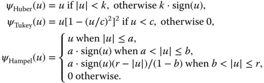
The parameters ![]() ,
, ![]() ,
, ![]() ,
, ![]() , and
, and ![]() are tuning parameters that determine the rate of increase as a function of
are tuning parameters that determine the rate of increase as a function of ![]() and the locations where
and the locations where ![]() levels off. Figure 10.4 shows the shape of the
levels off. Figure 10.4 shows the shape of the ![]() and
and ![]() functions of Huber, Tukey, and Hampel. The constants were chosen so that the regression estimators have an efficiency of 95% as described, for example, by Koller and Mächler (2016), that is,
functions of Huber, Tukey, and Hampel. The constants were chosen so that the regression estimators have an efficiency of 95% as described, for example, by Koller and Mächler (2016), that is, ![]() ,
, ![]() ,
, ![]() ,
, ![]() , and
, and ![]() , where
, where ![]() .
.

Figure 10.4 Three  - and
- and  -functions used in
  -estimation (plotted so that the scales of the
  axes are comparable). For comparison, the traditional function
  is plotted with dotted lines.
With the simputation package, imputation based on ![]() -estimated linear regression parameters can be done with the
-estimated linear regression parameters can be done with the impute_rlm function. It uses the ![]() function of the
function of the MASS package for coefficient estimation.
  impute_rlm(retl, turnover + other.rev + total.rev ∼ staff) %>% head(3)
  ##   size staff turnover other.rev total.rev vat
  ## 1  sc0    75 12927.56 159.16574      1130  NA
  ## 2  sc3     9  1607.00  16.29018      1607  NA
  ## 3  sc3    NA  6886.00 -33.00000      6919  NA
The default is to use Huber's ![]() function with
function with ![]() . Extra arguments are passed through to
. Extra arguments are passed through to rlm. For example, rlm has the option to set method="MM". This sets a number of options ensuring that the regression estimator has a high breakdown point (qualitatively, the fraction of outliers that may be present in the data before the estimator gives unacceptable results).
  impute_rlm(retl, turnover + other.rev + total.rev ∼ staff
   , method="MM") %>% head(3)
  ##   size staff turnover other.rev total.rev vat
  ## 1  sc0    75 13529.59  75.34900      1130  NA
  ## 2  sc3     9  1607.00  13.24304      1607  NA
  ## 3  sc3    NA  6886.00 -33.00000      6919  NA
10.3.4 Lasso, Ridge, and Elasticnet Regression
With impute_en, elasticnet regression is used to compute imputations. In linear elasticnet regression, the parameters are estimated as

where ![]() is the familiar Euclidean norm and
is the familiar Euclidean norm and ![]() the
the ![]() -norm or the sum over absolute values of the coefficients of its argument. The penalty term is defined in terms of
-norm or the sum over absolute values of the coefficients of its argument. The penalty term is defined in terms of ![]() , which denotes all coefficients except the intercept (when present). The parameter
, which denotes all coefficients except the intercept (when present). The parameter ![]() allows one to shift smoothly from ridge regression (
allows one to shift smoothly from ridge regression (![]() ) to lasso regression (
) to lasso regression (![]() ), while
), while ![]() determines the overall strength of the penalty. The characteristic difference between lasso and ridge regression is that in the case of correlated predictors, lasso regression tends to push one or more coefficients to zero, while ridge regression spreads the value of coefficients over multiple correlated variables.
determines the overall strength of the penalty. The characteristic difference between lasso and ridge regression is that in the case of correlated predictors, lasso regression tends to push one or more coefficients to zero, while ridge regression spreads the value of coefficients over multiple correlated variables.
The simputation package implements elasticnet imputation through the impute_en function, which depends on the glmnet package of Friedman et al. (2010).
  impute_en(retl, turnover + other.rev + total.rev ∼ staff + size
     , s=0.005, alpha=0.5) %>% head(3)
  ##   size staff turnover other.rev total.rev vat
  ## 1  sc0    75 13360.82 -8354.709      1130  NA
  ## 2  sc3     9  1607.00 10476.443      1607  NA
  ## 3  sc3    NA  6886.00   -33.000      6919  NA
Here, the predictor size is added since the glmnet package does not accept models with less than two predictors. The parameter s determines the size of the overall penalty factor ![]() used in predictions, and we (arbitrarily) set
used in predictions, and we (arbitrarily) set alpha=0.5.
10.3.5 Classification and Regression Trees
Decision tree models can be used in situations where the predicted variable is numeric and its dependence on the predictors is highly nonlinear, or when the predicted variable is categorical with probabilities that have complex dependence on predictor variables. In both the cases, the predictors can be numeric or categorical. Because decision tree models can be used to predict quantitative as well as qualitative variables, they are often referred to as classification and regression trees or CART, for short. The term was introduced by Breiman et al. (1984), and it also refers to a specific method for setting up the decision tree (which will be treated below).
Consider again a predicted variable ![]() (to be imputed) and a set of predictors
(to be imputed) and a set of predictors ![]() . The idea is to partition the set of all possible value combinations
. The idea is to partition the set of all possible value combinations ![]() into disjunct regions, such that the corresponding value of
into disjunct regions, such that the corresponding value of ![]() is as homogeneous as possible in each region. For numeric
is as homogeneous as possible in each region. For numeric ![]() , homogeneous usually means ‘a small variance’; for categorical data, it means ‘a high proportion of a single category’. Given a particular record
, homogeneous usually means ‘a small variance’; for categorical data, it means ‘a high proportion of a single category’. Given a particular record ![]() , one follows a binary decision tree
, one follows a binary decision tree ![]() to see in what region the record falls. The predicted value for numeric
to see in what region the record falls. The predicted value for numeric ![]() is then the mean value within the region (although more robust estimators are sometimes used as well), and the predicted value for categorical
is then the mean value within the region (although more robust estimators are sometimes used as well), and the predicted value for categorical ![]() is the category with the highest prevalence.
is the category with the highest prevalence.
Before considering how such a decision tree is constructed, consider the example of Figure 10.5. Here, we used the rpart package to build a predictive model for the staff variable in the retailers dataset. Depicted are two representations of the resulting model. In Figure 10.5(a), the decision tree is shown. Each nonterminal node contains two numbers and a decision rule. The root node represents 100% of the records, and the mean value for staff over all those records equals 12 (rounded). If we partition the dataset according to the rule total.rev < 3464, we get 83% records for which this rule holds, with a mean number of staff of 7.7 and 17% records for which this total.rev >= 3464, with a mean number of staff of 31. The latter case ends in a terminal node and thus corresponds with a single partition of the feature space. The group of records falling into this category are on the right of the second vertical line in Figure 10.5(b). The group of records on the left (with total.rev < 3464) are subdivided by having smaller or larger total.rev of 968. The latter are subdivided once more based on whether the size variable equals "sc2" (depicted in white in panel (b)). The terminal nodes of the tree contain the actual predictions made for each partition along with the size of the partition.

Figure 10.5 (a) A decision tree for estimating number of staff in the retailers dataset, computed with rpart. (b) The space partitioning. The vertical bars indicate the limits represented in the top node and the subdivision indicated by its left child node. In the middle region, white dots indicate records where size=="sc2".
When comparing this procedure with Eq. (10.5), we see that here, the model function is a procedure ![]() , that is parameterized by a decision tree
, that is parameterized by a decision tree ![]() . Based on the values of
. Based on the values of ![]() , the tree is traversed until a terminal node is reached and the prediction returned.
, the tree is traversed until a terminal node is reached and the prediction returned.
The tree itself is built up iteratively. Given a ![]() dataset
dataset ![]() and a set of values
and a set of values ![]() , the optimal split based on each variable
, the optimal split based on each variable ![]() is computed. Of those
is computed. Of those ![]() splits, the one resulting in the lowest error is chosen. This process is then repeated for each partition recursively. Note that for any dataset, it is in principle possible to create a perfect partition by growing the tree until each leaf has a single record in it (or only records with equal values for
splits, the one resulting in the lowest error is chosen. This process is then repeated for each partition recursively. Note that for any dataset, it is in principle possible to create a perfect partition by growing the tree until each leaf has a single record in it (or only records with equal values for ![]() ). In practice, one stops at some minimum number of records. The resulting (still large) tree is then pruned by removing leaf nodes from the bottom up. The final result is determined by a trade-off between error minimization and tree size
). In practice, one stops at some minimum number of records. The resulting (still large) tree is then pruned by removing leaf nodes from the bottom up. The final result is determined by a trade-off between error minimization and tree size ![]() :
:

Here, ![]() is the set of subtrees that can be obtained by pruning the initial tree. The function ‘error’ records the mismatch between prediction and observation, appropriate for the variable
is the set of subtrees that can be obtained by pruning the initial tree. The function ‘error’ records the mismatch between prediction and observation, appropriate for the variable ![]() (e.g., standard deviation for numerical variables end mismatch ratio for categorical variables). The term
(e.g., standard deviation for numerical variables end mismatch ratio for categorical variables). The term ![]() penalizes the number of nodes
penalizes the number of nodes ![]() . Here,
. Here, ![]() is referred to as the cost-complexity parameter. It is determined automatically by computing
is referred to as the cost-complexity parameter. It is determined automatically by computing ![]() for a series of values of
for a series of values of ![]() and applying cross-validation to select the best one [see also James et al. (2013, Chapter 8) or Hastie et al. (2001, Chapter 9)].
and applying cross-validation to select the best one [see also James et al. (2013, Chapter 8) or Hastie et al. (2001, Chapter 9)].
With the simputation package, CART-based imputation can be performed with the impute_cart. The specification of predictor variables tells impute_cart what variables can be used in the tree. In many cases, one can choose all variables except the predicted since decision trees have variable selection built-in.
  impute_cart(retl, staff ∼ .) %>% head(3)
  ##   size    staff turnover other.rev total.rev vat
  ## 1  sc0 75.00000       NA        NA      1130  NA
  ## 2  sc3  9.00000     1607        NA      1607  NA
  ## 3  sc3 30.66667     6886       -33      6919  NA
Imputation took place in the third record. The imputation value can be traced by following the decision tree of Figure 10.5. The total revenue in the third record equals 6919. Since this is larger than 3464, we end in a leaf node immediately and predict a value of 30.67.
One advantage of CART models over linear models for imputation is their resilience against missing values in predictors. For a linear model, the imputation ![]() cannot be estimated when any of the
cannot be estimated when any of the ![]() happens to be missing unless it is somehow imputed. In a CART model, the actual decision tree contains more information than shown in Figure 10.5. Anticipating on possible missing predictors, each node stores one or more backup split rules based on other predictors present in the dataset. If during prediction some value
happens to be missing unless it is somehow imputed. In a CART model, the actual decision tree contains more information than shown in Figure 10.5. Anticipating on possible missing predictors, each node stores one or more backup split rules based on other predictors present in the dataset. If during prediction some value ![]() is found to be missing, its first so-called surrogate variable is used to decide the split. If the surrogate is also missing, the next one is used, and so on, until an observed surrogate is found, or no surrogates are left. In the latter case, the most populated child node is chosen. The loss of quality of prediction is smaller when surrogates are highly correlated with the primary splitting variables.
is found to be missing, its first so-called surrogate variable is used to decide the split. If the surrogate is also missing, the next one is used, and so on, until an observed surrogate is found, or no surrogates are left. In the latter case, the most populated child node is chosen. The loss of quality of prediction is smaller when surrogates are highly correlated with the primary splitting variables.
10.3.6 Random Forest
Random forest (Breiman, 2001) is an ensemble-based improvement over CART. It can be used to predict both qualitative and quantitative variables. The idea is to take bootstrap samples from the original data, and grow a decision tree for each sample. Moreover, at each split, a subset of the ![]() available predictors (typically about
available predictors (typically about ![]() is randomly chosen as possible splitting variables. Randomizing the available splitting variables is used to decrease correlation between the trees.
is randomly chosen as possible splitting variables. Randomizing the available splitting variables is used to decrease correlation between the trees.
Training a random forest model thus results in a set of ![]() trees
trees ![]() called a forest. If the predicted variable is numerical, the prediction is an aggregate over the individual predictions such as the mean,
called a forest. If the predicted variable is numerical, the prediction is an aggregate over the individual predictions such as the mean,

but in principle, it is possible to use a robust aggregate such as the median as well. For categorical variables, the majority vote over the trees is taken.
With the simputation package, random forest models can be employed for imputation as follows:
  impute_rf(retl, staff ∼ .) %>% head(3)
  ##   size staff turnover other.rev total.rev vat
  ## 1  sc0    75       NA        NA      1130  NA
  ## 2  sc3     9     1607        NA      1607  NA
  ## 3  sc3    NA     6886       -33      6919  NA
Random forest models are somewhat less resilient against missing predictors than the CART models discussed in the previous paragraph. The underlying Fortran code by Breiman and Cutler (2004) is able to use a rough imputation scheme on the training set to generate the forest (this can be set by passing na_action=na.rough fix; this will impute medians for numeric data and modes for categorical data). For prediction, however, not every variable needs to be present: the average can be taken over the subset of trees that do return a value. However, for small datasets such as in this example, it may occur that all trees return NA so no prediction is possible. Here, the problem can be partially resolved by removing a variable with little observations from the list of predictors.
  impute_rf(retl, staff ∼ . - vat) %>% head(3)
  ##   size    staff turnover other.rev total.rev vat
  ## 1  sc0 75.00000       NA        NA      1130  NA
  ## 2  sc3  9.00000     1607        NA      1607  NA
  ## 3  sc3 20.23483     6886       -33      6919  NA
Besides simputation, there are other R packages implementing imputation based on random forests. The missForest package by Stekhoven and Bühlmann (2012) implements an iterative imputation procedure. For initiation, missing values get imputed using a simple rule. Next, a random forest is trained on the completed dataset, yielding updated imputation values. This second step is repeated until a convergence criterion has been satisfied. When installed, the missForest package can be interfaced via simputation using impute_mf.
  impute_mf(retl, staff ∼ .) %>% head(3)
  ##   missForest iteration 1 in progress…done!
  ##   missForest iteration 2 in progress…done!
  ##   size staff turnover other.rev total.rev vat
  ## 1  sc0 75.00       NA        NA      1130  NA
  ## 2  sc3  9.00     1607        NA      1607  NA
  ## 3  sc3 18.15     6886       -33      6919  NA
Here, all variables are imputed (iteratively) and used as predictors, but only the variables on the left-hand side for the formula are copied to the resulting dataset. With the formula . ∼ . all variables can be imputed.
10.4 Donor Imputation with R
In donor imputation, a missing value in one record is replaced with an observed value that is copied from another and somehow otherwise similar record. The record from which the value is copied is referred to as the ‘donor’ record; hence, the name of the method. Donor imputation is also referred to as hot deck imputation. The etymology of this term derives from the state of the art in computing when the method was first applied. Researchers would ‘hot deck impute’ by drawing from a deck of computer punch cards representing records (Andridge and Little, 2010; Cranmer and Gill, 2013).
When compared to model-based imputation, the advantage of donor imputation is that the imputed value is always an actually existing (observed) value. Statistical models always run the risk of predicting a value that is not (physically) possible, especially when extrapolating beyond the observed range of values. The downside of donor imputation is that in spite of its wide application, theoretical underpinning is not as strong as for model-based methods. Moreover, Andridge and Little (2010) conclude in their extensive review that no consensus exists on the best way to apply hot deck imputation methods, and note that ‘many multivariate hot deck methods seem relatively ad hoc’. Nevertheless, hot deck methods have been commonly applied for a long time in areas related to official statistics [see Ono and Miller (1969); Bailar and Bailar (1979); and Cox (1980) for some early applications and method comparisons] and to a lesser extend in medical or epidemiological settings. Method comparisons are given in, for example, Barzi and Woodward (2004); Engels and Diehr (2003); Perez et al. (2002); Reilly and Pepe (1997); Tang et al. (2005), and Twisk and de Vente (2002).
Hot deck imputation methods are commonly categorized along two dimensions. The first dimension distinguishes between methods where multiple missing values in a record are imputed from the same donor (multivariate donor imputation) and methods where a separate donor may be appointed for each missing variable. The main advantage of multivariate donor imputation is that one only imputes valid and existing value combinations, so that imputed values cannot introduce inconsistencies. The downside is that the number of possible donors may be greatly reduced as the number of missing values in a record increases. The hot deck donor imputation routines in simputation have an option called pool, which control this behavior. Its possible values are
"complete": |
Use only complete records as donor pool and perform multivariate imputation. This is the default |
"univariate": |
A new donor is sought for each variable. |
"multivariate": |
For each occurring pattern of missingness find suitable donors and perform multivariate imputation. |
The second dimension distinguishes between the various ways donor records are determined, and each of these methods (discussed next) can be executed in a univariate or multivariate fashion.
10.4.1 Random and Sequential Hot Deck Imputation
In random hot deck imputation, a donor is sampled from a donor pool. Often, a dataset is separated into imputation cells for which one or more auxiliary variables have the same values. With the simputation package, the imputation cells are determined by the right-hand side of the formula object specifying the model (we continue with the retl dataset constructed in the previous paragraph).
  set.seed(1) # make reproducible
  # random hot deck imputation (multivariate; complete cases are donor)
  impute_rhd(retl, turnover + other.rev + total.rev ∼ size) %>% head(3)
  ##   size staff turnover other.rev total.rev vat
  ## 1  sc0    75      359         9      1130  NA
  ## 2  sc3     9     1607     98350      1607  NA
  ## 3  sc3    NA     6886       -33      6919  NA
In the above example, the dataset is split according to the size class label, and data are imputed in univariate manner. That is, for each variable, a value is sampled from all observed values within the same size class. If multiple categorical variables are used to define imputation cells, the donor pools can quickly decrease in size, leading possibly to many imputations of the same value. Setting pool="univariate" can alleviate this issue to a small extend since per-variable donor pools are generally larger than multivariate donor pools.
  # random hot deck imputation (univariate)
  impute_rhd(retl, turnover + other.rev + total.rev ∼ size
   , pool="univariate") %>% head(3)
  ##   size staff turnover other.rev total.rev vat
  ## 1  sc0    75      197       622      1130  NA
  ## 2  sc3     9     1607        33      1607  NA
  ## 3  sc3    NA     6886       -33      6919  NA
By default, records are drawn uniformly from the pool, but one can pass a numeric vector prob assigning a probability to each record in the imputed data. Probabilities will be rescaled as necessary, depending on grouping and donor pool specification.
In sequential hot deck, one sorts the dataset using one or more variables, and missing values in a record are taken from the first preceding or ensuing record that has a value. If values are taken from preceding records, the method is referred to as last observation carried forward or LOCF in short, if values are taken from ensuing records, the method is referred to as next observation carried backward (NOCB). With the simputation package, sequential hot deck is executed with the impute_shd function. The ‘predictor variables’ in the formula are used to sort the data (with every variable after the first used as tie-breaker for the previous one).
  impute_shd(retl, turnover + other.rev + total.rev ∼ staff) %>% head(3)
  ##   size staff turnover other.rev total.rev vat
  ## 1  sc0    75     9067       622      1130  NA
  ## 2  sc3     9     1607        38      1607  NA
  ## 3  sc3    NA     6886       -33      6919  NA
The sort order is always ‘increasing’, but with the argument order, one can choose to use between "nocb" (the default) and "locb" imputation.
Both random and sequential hot decks are implemented in the simputation source code. Especially for large datasets and many groups, it is beneficial to use the faster implementation provided by the VIM package. This is possible for both impute_rhd and impute_shd by setting backend="VIM". Options specific to simputation (such as the order argument) will be ignored, but one can pass any argument of VIM::hotdeck to impute_rhd or impute_shd for detailed control over the imputation method.
10.4.2  Nearest Neighbors and Predictive Mean Matching
In the ![]() -nearest-neighbor (knn) method, a similarity measure is used to find the knns to a record containing missing values. Next, a donor value is determined. Donor value determination can be done by randomly selecting from the
-nearest-neighbor (knn) method, a similarity measure is used to find the knns to a record containing missing values. Next, a donor value is determined. Donor value determination can be done by randomly selecting from the ![]() neighbors or, for example (in the case of categorical data), by choosing the majority value. A particularly popular similarity measure is that of Gower (1971). Given two records
neighbors or, for example (in the case of categorical data), by choosing the majority value. A particularly popular similarity measure is that of Gower (1971). Given two records ![]() and
and ![]() , each with
, each with ![]() variables that may be numeric, categorical, or missing, Gower's similarity measure
variables that may be numeric, categorical, or missing, Gower's similarity measure ![]() can be written as
can be written as

The values of ![]() and
and ![]() depend on the variable type. If the
depend on the variable type. If the ![]() th variable is numeric, then
th variable is numeric, then

Here, ![]() is the observed range of the
is the observed range of the ![]() th variable. If the
th variable. If the ![]() th variable is categorical, then
th variable is categorical, then ![]() is defined as
is defined as
For numerical and categorical variables, the importance weights ![]() may be chosen at will, but they are usually set to 1 or 0, where setting
may be chosen at will, but they are usually set to 1 or 0, where setting ![]() amounts to excluding the
amounts to excluding the ![]() th variable from the similarity calculation. For a dichotomous (
th variable from the similarity calculation. For a dichotomous (logical, in R) variable, ![]() is yet defined differently, namely,
is yet defined differently, namely,
while the weights are defined as
Here, we identify the logical outputs true with 1 and false with 0. The rationale is that a dichotomous variable only adds to the similarity when both variables are true. If any of the two variables is true they add to the weight in the denominator.
In the simputation package, knn imputation based on Gower's similarity is performed with the impute_knn function. The predictor variables in the formula argument specify which variables are used to determine Gower's similarity. Below, we use all variables by specifying the dot (.). The default value for ![]() , but by setting
, but by setting ![]() , values are copied directly from the nearest neighbor.
, values are copied directly from the nearest neighbor.
  impute_knn(retl, turnover + other.rev + total.rev ∼ ., k=1) %>% head(3)
  ##   size staff turnover other.rev total.rev vat
  ## 1  sc0    75     9067       622      1130  NA
  ## 2  sc3     9     1607        13      1607  NA
  ## 3  sc3    NA     6886       -33      6919  NA
Like for the random and sequential hot deck imputation procedures, the donor pool can be specified ("complete", "univariate", or "multivariate") and the VIM package can be used as computational backend.
Predictive mean matching (PMM) is a nearest-neighbor imputation method where the donor is determined by comparing predicted donor values with model-based predictions for the recipient's missing values. It can therefore be seen as a method that lies between the purely model-based and purely donor-based imputation methods. On one hand, it partially shares the benefits of both approaches, utilizing the power of predictive modeling while making sure only observed values are imputed. On the other hand, it inherits some of the intricacies of both worlds, such as issues with model selection and the possibility of small donor pools. In practice, PMM has become a popular method, and the popular mice package for multiple imputation (van Buuren and Groothuis-Oudshoorn, 2011) uses it as default imputation method.
In simputation, PMM is achieved with the impute_pmm function. Besides the data to be imputed and a predictive model-specifying formula, it takes one of the impute_ functions as an argument to preimpute the recipients with a chosen model. By default, impute_lm is used so the formula object must specify a linear model.
  impute_pmm(retl, turnover + other.rev + total.rev ∼ staff) %>% head(3)
  ##   size staff turnover other.rev total.rev vat
  ## 1  sc0    75     7271        30      1130  NA
  ## 2  sc3     9     1607      1831      1607  NA
  ## 3  sc3    NA     6886       -33      6919  NA
However, one can switch to a robust linear model based on the ![]() -estimator as follows:
-estimator as follows:
  impute_pmm(retl, turnover + other.rev + total.rev ∼ staff
   , predictor=impute_rlm, method="MM") %>% head(3)
  ##   size staff turnover other.rev total.rev vat
  ## 1  sc0    75     9067       622      1130  NA
  ## 2  sc3     9     1607        13      1607  NA
  ## 3  sc3    NA     6886       -33      6919  NA
10.5 Other Methods in the simputation Package
There are a few other imputation approaches supported by the simputation package that facilitate certain type of imputations.
The first method is a utility function allowing to replace missing values with a constant. For example,
  impute_const(retl, other.rev ∼ 0) %>% head(3)
  ##   size staff turnover other.rev total.rev vat
  ## 1  sc0    75       NA         0      1130  NA
  ## 2  sc3     9     1607         0      1607  NA
  ## 3  sc3    NA     6886       -33      6919  NA
Such an imputation strategy implies strong assumptions that in some cases may nevertheless be reasonable. For example, one could assume that values that are not submitted by a respondent can be interpreted as ‘not applicable’ or in this case zero. Obviously, one should very carefully test such an assumption since they can introduce severe bias in estimates based on the data.
The second method is referred to by de Waal et al. (2011) as proxy imputation. Here, the missing value is estimated by copying a value from the same record, but from another variable. For example, we may estimate the variable total turnover in the retailers dataset by copying the amount of turnover reported to the tax office for vat.
  impute_proxy(retl, total.rev ∼ vat) %>% head(3)
  ##   size staff turnover other.rev total.rev vat
  ## 1  sc0    75       NA        NA      1130  NA
  ## 2  sc3     9     1607        NA      1607  NA
  ## 3  sc3    NA     6886       -33      6919  NA
This method is useful only when both the economic definition of turnover and the legal definition used by the tax authorities coincide or are very close.
The simputation package is more flexible than De Waal et al.'s original definition and also allows for imputing functions of variables.
  impute_proxy(retl
   , turnover ∼ mean(turnover/total.rev,na.rm=TRUE) * total.rev) %>%
    head(3)
  ##   size staff turnover other.rev total.rev vat
  ## 1  sc0    75 1351.159        NA      1130  NA
  ## 2  sc3     9 1607.000        NA      1607  NA
  ## 3  sc3    NA 6886.000       -33      6919  NA
Here, the right-hand side of the formula may evaluate to a vector of unit length or to a vector with length equal to the number of input rows. Proxy imputation also accepts grouping, so imputing the group mean can be done as follows:
  impute_proxy(retl, turnover ∼ mean(turnover, na.rm=TRUE) | size)
  %>% head(3)
  ##   size staff turnover other.rev total.rev vat
  ## 1  sc0    75 1420.375        NA      1130  NA
  ## 2  sc3     9 1607.000        NA      1607  NA
  ## 3  sc3    NA 6886.000       -33      6919  NA
10.6 Imputation Based on the EM Algorithm
The purpose of the Expectation–Maximization algorithm (Dempster et al., 1977) is to estimate the maximum-likelihood estimate for parameters of a multivariate probability distribution in the presence of missing data. As such, it is not an imputation method. Imputations can be generated by computing the expected value for missing items conditional on the observed data or by sampling them from the conditional multivariate distribution.
Contrary to the model-based imputation methods discussed up until now, in the EM algorithm, there is no fixed distinction between predicting and predicted variables—one simply uses everything available to estimate the parameters of some model distribution. This also means that one needs to assume a distributional form (e.g., multivariate normal) for the combined variables in the dataset.
10.6.1 The EM Algorithm
Consider again a set of random variables ![]() with a joint probability distribution
with a joint probability distribution ![]() parameterized by a numeric vector
parameterized by a numeric vector ![]() . We denote a realization of
. We denote a realization of ![]() as a row vector
as a row vector ![]() and a set of
and a set of ![]() realizations as a
realizations as a ![]() matrix
matrix ![]() . A common way to estimate the parameters of
. A common way to estimate the parameters of ![]() given a set of observations is to assume a distributional form for
given a set of observations is to assume a distributional form for ![]() (say, multinormal) and then solve the following maximization problem.
(say, multinormal) and then solve the following maximization problem.

where ![]() is the space of possible values for
is the space of possible values for ![]() . Furthermore, we used Bayes' rule in the second line, and in the third line, we used that taking the logarithm does not alter the location of the maximum. If there is no prior knowledge about
. Furthermore, we used Bayes' rule in the second line, and in the third line, we used that taking the logarithm does not alter the location of the maximum. If there is no prior knowledge about ![]() , we may assume that
, we may assume that ![]() is uniformly distributed over
is uniformly distributed over ![]() , so
, so ![]() is constant. Since
is constant. Since ![]() is also independent of
is also independent of ![]() , the maximization problem can be simplified to
, the maximization problem can be simplified to
where we introduced the notation ![]() , which is referred to as the maximum-likelihood function. Correspondingly, Eq. (10.10) is referred to as the maximum-likelihood estimator. It returns the value of
, which is referred to as the maximum-likelihood function. Correspondingly, Eq. (10.10) is referred to as the maximum-likelihood estimator. It returns the value of ![]() such that
such that ![]() is the most likely observed data. To actually solve this equation, one substitutes a distribution (e.g., multinormal), equates the right-hand side to zero, and solves for
is the most likely observed data. To actually solve this equation, one substitutes a distribution (e.g., multinormal), equates the right-hand side to zero, and solves for ![]() .
.
If only part of the realizations ![]() are actually observed, this maximization problem cannot be solved. To move forward, we partition
are actually observed, this maximization problem cannot be solved. To move forward, we partition ![]() into the observed values
into the observed values ![]() and missing values
and missing values ![]() . Using Bayes' rule twice, we can write
. Using Bayes' rule twice, we can write

Again, dropping terms not depending on ![]() (and we already assumed that
(and we already assumed that ![]() is constant), we find that maximizing the likelihood function of Eq. (10.10) can equivalently be written as the maximization over the likelihood function
is constant), we find that maximizing the likelihood function of Eq. (10.10) can equivalently be written as the maximization over the likelihood function
Since ![]() is unknown, this expression cannot be maximized. The idea of Dempster et al. (1977) is to replace the maximum-likelihood function with its expected value with regard to the missing values.
is unknown, this expression cannot be maximized. The idea of Dempster et al. (1977) is to replace the maximum-likelihood function with its expected value with regard to the missing values.

Here, integration is over all unobserved variables, where ![]() indicates the domain of possible values for the variables in
indicates the domain of possible values for the variables in ![]() . In the second line, Eq. (10.11) was substituted. The integral in the second line is the negative entropy of the distribution
. In the second line, Eq. (10.11) was substituted. The integral in the second line is the negative entropy of the distribution ![]() . It is therefore usually denoted
. It is therefore usually denoted ![]() . In principle, one can numerically maximize the above expression to obtain
. In principle, one can numerically maximize the above expression to obtain ![]() . However, if
. However, if ![]() has a simple form, and we choose some value
has a simple form, and we choose some value ![]() , the integral
, the integral

can often be worked out explicitly. Next, an updated value for ![]() can be found by maximizing
can be found by maximizing ![]() as a function of
as a function of ![]() . The Expectation–Maximization algorithm is indeed an iteration over this procedure. The crucial result of Dempster et al. (1977) is that the value of
. The Expectation–Maximization algorithm is indeed an iteration over this procedure. The crucial result of Dempster et al. (1977) is that the value of ![]() must increase at each iteration and converge to a maximum under mild conditions, including cases where
must increase at each iteration and converge to a maximum under mild conditions, including cases where ![]() is a member of the regular exponential family.
is a member of the regular exponential family.
If ![]() is a member of the regular exponential family, the expressions to be evaluated by the algorithm can be simplified by expressing them in terms of (expected values of) sufficient statistics [e.g., de Waal et al. (2011, Chapter 8) or Schafer (1997, Chapter 5)]. The regular exponential family includes a wide range of commonly applied distributions including the (multivariate) normal, Bernoulli, exponential, (negative) binomial, Poisson, and gamma distributions [see, e.g., Brown (1986)]. Indeed, many implementations of the EM algorithm demand that
is a member of the regular exponential family, the expressions to be evaluated by the algorithm can be simplified by expressing them in terms of (expected values of) sufficient statistics [e.g., de Waal et al. (2011, Chapter 8) or Schafer (1997, Chapter 5)]. The regular exponential family includes a wide range of commonly applied distributions including the (multivariate) normal, Bernoulli, exponential, (negative) binomial, Poisson, and gamma distributions [see, e.g., Brown (1986)]. Indeed, many implementations of the EM algorithm demand that ![]() is from the regular exponential family. The
is from the regular exponential family. The Amelia package discussed below is restricted to models based on the multivariate normal distribution.
Advantages of the EM algorithm include that it is a simple and well-understood algorithm that is guaranteed to converge in principle. Given a distribution from the exponential family, the E and M steps can be computed very quickly. Also, since the algorithm provides an estimate for the full multivariate distribution, it has a good chance of correcting for the random (MAR) mechanism. A disadvantage is that computation may take many iterations since the convergence criterion (measured in terms of the difference in ![]() between iterations) decreases approximately linearly with the number of iterations (Schafer, 1997). Convergence can be especially slow when the fraction of missing values is high or when the model distribution is a poor description of the actual data distribution. Furthermore, the EM algorithm does not immediately provide a variance estimate for
between iterations) decreases approximately linearly with the number of iterations (Schafer, 1997). Convergence can be especially slow when the fraction of missing values is high or when the model distribution is a poor description of the actual data distribution. Furthermore, the EM algorithm does not immediately provide a variance estimate for ![]() .
.
10.6.2 EM Imputation Assuming the Multivariate Normal Distribution
Probably, one of the most implemented models for EM estimation is the model where numeric variables are distributed according to the multivariate normal distribution. This distribution is parameterized by the mean vector ![]() and covariance matrix
and covariance matrix ![]() , with the probability density function given by
, with the probability density function given by

Because of its relatively simple form, the update rules for the E and M steps can be worked out yielding expressions that eventually be evaluated using simple matrix algebra and linear system solving.
Before stating the algorithm, consider a record ![]() with observed values
with observed values ![]() and missing values
and missing values ![]() . Given an estimate for the mean vector and covariance matrix, these can be rearranged accordingly, so
. Given an estimate for the mean vector and covariance matrix, these can be rearranged accordingly, so

Here, ![]() is the estimated covariance matrix for observed variables,
is the estimated covariance matrix for observed variables, ![]() the estimated covariance matrix between observed and missing variables, and
the estimated covariance matrix between observed and missing variables, and ![]() the estimated covariance matrix for the missing variables. After a fair amount of tedious algebra and integration, one can show that the expected value(s) for the missing part of
the estimated covariance matrix for the missing variables. After a fair amount of tedious algebra and integration, one can show that the expected value(s) for the missing part of ![]() conditional on
conditional on ![]() ,
, ![]() , and
, and ![]() is given by
is given by
This equation can be used to impute a record once the parameters have been estimated (Procedure 10.6.2). The imputed dataset is obtained by applying Eq. (10.12) one last time on every record in the dataset.
  impute_em(retl, ∼ .- size) %>% head(3)
  ##   size    staff  turnover other.rev total.rev      vat
  ## 1  sc0 75.00000  893.2151  1168.523      1130 7917.634
  ## 2  sc3  9.00000 1607.0000  4373.896      1607 1749.444
## 3 sc3 11.84416 6886.0000 -33.000 6919 1991.73010.7 Sampling Variance under Imputation
The goal of data analysis is often to infer the value of a population parameter, say ![]() . If the data is obtained by sampling from the population, an estimate
. If the data is obtained by sampling from the population, an estimate ![]() is obtained by applying some procedure to the observed dataset. In such cases, one is often interested in how much the estimator
is obtained by applying some procedure to the observed dataset. In such cases, one is often interested in how much the estimator ![]() would vary if the sampling-and-estimation procedure was to be repeated on the same population. The variation over all possible samples is usually measured by the sampling variance.
would vary if the sampling-and-estimation procedure was to be repeated on the same population. The variation over all possible samples is usually measured by the sampling variance.
Suppose that the parameter of interest is the population mean ![]() of a variable
of a variable ![]() . Given a sample, obtained using simple random sample without replacement, an unbiased estimate
. Given a sample, obtained using simple random sample without replacement, an unbiased estimate ![]() can be obtained by computing the sample mean. The sampling variance of
can be obtained by computing the sample mean. The sampling variance of ![]() , estimated from the same sample, is given by the well-known expression
, estimated from the same sample, is given by the well-known expression

where ![]() and
and ![]() are the sample and population size and
are the sample and population size and ![]() the observed sample values.
the observed sample values.
The important thing to realize here is that the expression for sampling variance depends on the sampling scheme (including size) and the expression or procedure used to obtain the estimator. This means that if part of the sampled data must be imputed, this imputation procedure should be considered part of the estimation procedure. This is easy to see from the abovementioned example. Suppose that some fraction of the observations ![]() are missing completely at random, and we impute them with the estimated mean (ignoring missing values). This clearly leads to negatively biased variance estimation since the terms in the sum of Eq. (10.13) corresponding to missing
are missing completely at random, and we impute them with the estimated mean (ignoring missing values). This clearly leads to negatively biased variance estimation since the terms in the sum of Eq. (10.13) corresponding to missing ![]() are zero by definition.
are zero by definition.
More generally, suppose that we are interested in some population parameter ![]() . Suppose further that estimation of
. Suppose further that estimation of ![]() includes some model-based imputation procedure depending on model parameters
includes some model-based imputation procedure depending on model parameters ![]() that are estimated from the same sample as
that are estimated from the same sample as ![]() . Using the rule of conditional variances (sometimes called Eve's law), we can write
. Using the rule of conditional variances (sometimes called Eve's law), we can write
If the sampling variance of ![]() is assumed to be zero or very small, the second term vanishes, and we get
is assumed to be zero or very small, the second term vanishes, and we get ![]() . The first term can therefore be interpreted as the sampling variance of
. The first term can therefore be interpreted as the sampling variance of ![]() that is intrinsic to the sampling scheme, where the procedure to estimate
that is intrinsic to the sampling scheme, where the procedure to estimate ![]() includes imputation. The second term corresponds to variance added by uncertainty in the imputation model parameters.
includes imputation. The second term corresponds to variance added by uncertainty in the imputation model parameters.
The assumption that ![]() does not vary is valid in the case of imputations that do not vary with sample composition. This is the case, for example, when imputing with a fixed value or when using a deductive method such as those described in Section 9.3.2. Recall that in deductive methods one derives imputed values from conditions on the data and observed values that are deemed valid. It is also valid when the model used to impute the data was fitted on a dataset that is different from the imputed dataset (but note that this may bias the estimator since one assumes that model parameters are constant across datasets).
does not vary is valid in the case of imputations that do not vary with sample composition. This is the case, for example, when imputing with a fixed value or when using a deductive method such as those described in Section 9.3.2. Recall that in deductive methods one derives imputed values from conditions on the data and observed values that are deemed valid. It is also valid when the model used to impute the data was fitted on a dataset that is different from the imputed dataset (but note that this may bias the estimator since one assumes that model parameters are constant across datasets).
In many common cases the assumption of zero variation in imputation model parameters will be invalid, and hence the second term in Eq. (10.14) will be positive. In particular, any procedure where a dataset is imputed using a predictive model, which is subsequently ignored in variance estimation, will underestimate the sampling variance.
Over the past decades, two contrasting views of variance estimation over partially imputed datasets have developed. The first, historically, is due to Rubin who published and refined methodology for multiple imputation over several publications [see Rubin (1978); Rubin (1996); and the basic reference Rubin (1987)]. Rubin (1978) proposes to impute each missing data multiple times so as to ‘reflect variation within a model as well as [![]() ] due to a variety of reasonable models’. An analyst who is assumed to be not involved in the imputation process can get an idea of the variance due to imputation by computing parameters of interest over several copies of the imputed dataset.
] due to a variety of reasonable models’. An analyst who is assumed to be not involved in the imputation process can get an idea of the variance due to imputation by computing parameters of interest over several copies of the imputed dataset.
The second view was proposed first by Rao and Shao (1992) in the context of hot deck imputation, but the idea applies more generally. In their view, one considers a population parameter ![]() , which is in the complete data case estimated by
, which is in the complete data case estimated by ![]() . As usual, the estimated quantity has an associated (estimated) sampling variance, denoted
. As usual, the estimated quantity has an associated (estimated) sampling variance, denoted ![]() (recall that the sampling variance is caused by variation of
(recall that the sampling variance is caused by variation of ![]() over all possible same-sized samples from a population). In the case of missing data, the estimator
over all possible same-sized samples from a population). In the case of missing data, the estimator ![]() is replaced with
is replaced with ![]() , which is similar to
, which is similar to ![]() except that it is applied to the imputed dataset. Based on a resampling formalism (the jackknife), they are able to define and analytically approximate an estimator for the sampling variance
except that it is applied to the imputed dataset. Based on a resampling formalism (the jackknife), they are able to define and analytically approximate an estimator for the sampling variance ![]() .
.
An account of both methodologies and arguments for and against these approaches is given in Rao (1996), Rubin (1996), and Fay (1996) and the ensuing comments by Judkins (1996), Binder (1996), and Eltinge (1996). In the following paragraphs, both methods are discussed in some detail.
10.8 Multiple Imputations
Multiple imputation is a computational method that allows for direct estimation of the two variance components of Eq. (10.14). A schematic of the main idea is shown in Figure 10.6. We start on the left-hand side with a (possibly multivariate) dataset ![]() of which some fraction of values are missing. This dataset is imputed
of which some fraction of values are missing. This dataset is imputed ![]() times, independently using an imputation model where both the model parameters and the imputed values are drawn from a distribution that is conditioned on the model's predictor variables. Each dataset is then used to estimate a population parameter
times, independently using an imputation model where both the model parameters and the imputed values are drawn from a distribution that is conditioned on the model's predictor variables. Each dataset is then used to estimate a population parameter ![]() using the same procedure one would use on
using the same procedure one would use on ![]() if it were complete to begin with. This yields an ensemble of estimates
if it were complete to begin with. This yields an ensemble of estimates ![]() . The final estimate is then computed as the average over the ensemble:
. The final estimate is then computed as the average over the ensemble:


Figure 10.6 Estimation using multiple imputation.
Similarly, one can estimate the variance for each estimate ![]() as one would for a complete sample. For example, if
as one would for a complete sample. For example, if ![]() is the mean of a variable, and
is the mean of a variable, and ![]() is obtained from simple random sampling without replacement, one could use Expression (10.13). This exercise then yields an ensemble of estimated variances
is obtained from simple random sampling without replacement, one could use Expression (10.13). This exercise then yields an ensemble of estimated variances ![]() . Averaging over this ensemble estimates the first term in Eq. (10.14), the expected value of the variance of
. Averaging over this ensemble estimates the first term in Eq. (10.14), the expected value of the variance of ![]() . The second term of Eq. (10.14)—the variance of the expected value—is estimated as the variance over the estimates
. The second term of Eq. (10.14)—the variance of the expected value—is estimated as the variance over the estimates ![]() . Combining the two estimates, we get (Rubin, 1987)
. Combining the two estimates, we get (Rubin, 1987)

where the term ![]() is a correction for the finite number of multiple imputations. In the context of multiple imputation, the first term is often referred to as within-imputation variance and the second term as the between-imputation variance.
is a correction for the finite number of multiple imputations. In the context of multiple imputation, the first term is often referred to as within-imputation variance and the second term as the between-imputation variance.
An advantage of the multiple imputation method is that it separates the imputation problem from later analysis and estimation. In fact, one of the aims of its development was to provide a way for data providers to impute a dataset such that analysts can use it for any statistical inference without knowing the details of the imputation method. The trade-off is then that an analyst must repeat the analysis ![]() times and appropriately combine the results.
times and appropriately combine the results.
This luxury of separating imputation from analysis does not come for free, however. As it turns out, it is not possible to choose the imputation method completely independent from the parameters being estimated. In essence, the imputation method must be such that the ![]() and
and ![]() (computed from imputed datasets) are unbiased estimates compared to the estimator one would use if
(computed from imputed datasets) are unbiased estimates compared to the estimator one would use if ![]() was observed completely. Furthermore, the between-imputation variance of
was observed completely. Furthermore, the between-imputation variance of ![]() must be an unbiased estimator of the variance caused by uncertainty in the model parameters (Rubin, 1987 1996). Imputations that satisfy these demands are called proper imputations [for a proper technical definition, cf. Rubin (1987)]. The demand for proper imputations therefore implies that imputation is not fully decoupled from analysis and that one needs to carefully design the imputation methods.
must be an unbiased estimator of the variance caused by uncertainty in the model parameters (Rubin, 1987 1996). Imputations that satisfy these demands are called proper imputations [for a proper technical definition, cf. Rubin (1987)]. The demand for proper imputations therefore implies that imputation is not fully decoupled from analysis and that one needs to carefully design the imputation methods.
A typical improper imputation method is imputation of the mean. Although this does yield an unbiased point estimate of the population mean, estimation of the sampling variance will be negatively biased. However, if the imputed variable is strongly correlated with one of the observed variables, this bias can be reduced with regression. The typical approach to multiple imputation is therefore an attempt to utilize as much as possible all relations between the variables so as to approximate the full multivariate distribution. Two such approaches will be discussed in the following sections: a bootstrapped version of the EM algorithm in Sections 10.8.1 and 10.8.2 and multivariate imputation by chained equations in Sections 10.8.3 and 10.8.4.
A natural question to ask is how large a value of ![]() is necessary. A value often quoted in the literature is
is necessary. A value often quoted in the literature is ![]() when the fraction of missing information
when the fraction of missing information ![]() is a few percent at most. This recommendation is based on an analysis of the efficiency1 of an estimator, which Rubin (1987) shows to be approximately equal to
is a few percent at most. This recommendation is based on an analysis of the efficiency1 of an estimator, which Rubin (1987) shows to be approximately equal to ![]() relative to the
relative to the ![]() case. Graham et al. (2007) performed extensive simulations to study the effect of
case. Graham et al. (2007) performed extensive simulations to study the effect of ![]() on the statistical power of an estimator rather than its efficiency. Based on the simulations where the parameter of interest concerned regression coefficients between a constructed pair of random normal variables, they conclude that drop-off in statistical power2 is much faster than is to be suspected from the drop-off in efficiency as
on the statistical power of an estimator rather than its efficiency. Based on the simulations where the parameter of interest concerned regression coefficients between a constructed pair of random normal variables, they conclude that drop-off in statistical power2 is much faster than is to be suspected from the drop-off in efficiency as ![]() decreases. They therefore recommend to use much higher numbers of imputations.
decreases. They therefore recommend to use much higher numbers of imputations.
Table 10.1 reproduces the recommendations of Graham et al. (2007). In the case of ![]() power loss compared to
power loss compared to ![]() , one would need to impute 20 times. A comparison with the full information maximum-likelihood model (FIML, which in their simulation is equivalent to the multivariate normal EM algorithm) is also made. The latter model may be considered a benchmark for their simulation when
, one would need to impute 20 times. A comparison with the full information maximum-likelihood model (FIML, which in their simulation is equivalent to the multivariate normal EM algorithm) is also made. The latter model may be considered a benchmark for their simulation when ![]() . When interpreting Table 10.1, one should keep in mind that it was produced based on artificial multivariate normal data. The number of necessary imputations may vary depending on the shape of the (multivariate) distribution and (possibly nonlinear) relations between the variables. In practice, one will therefore often need to experiment and gain experience with values for
. When interpreting Table 10.1, one should keep in mind that it was produced based on artificial multivariate normal data. The number of necessary imputations may vary depending on the shape of the (multivariate) distribution and (possibly nonlinear) relations between the variables. In practice, one will therefore often need to experiment and gain experience with values for ![]() that are appropriate for a particular imputation problem.
that are appropriate for a particular imputation problem.
Table 10.1 Number of multiple imputations ![]() , as recommended by Graham et al. (2007)
, as recommended by Graham et al. (2007)
| Acceptable power falloff | |||||
| Compared to |
Compared to EM | ||||
| 0.1 | 3 | 5 | 20 | 20 | |
| 0.3 | 10 | 20 | 20 | 20 | |
| 0.5 | 10 | 20 | 40 | 40 | |
| 0.7 | 20 | 40 | 40 | 100 | |
| 0.9 | 40 | 40 | 100 | >100 | |
![]() is the fraction of missing information, which equals the fraction of missing data when variables are independent.
is the fraction of missing information, which equals the fraction of missing data when variables are independent.
10.8.1 Multiple Imputation Based on the EM Algorithm
Honaker et al. (2011) propose a bootstrapping scheme to randomize the parameters for a multivariate normal model distribution. The idea, summarized in Procedure 10.8.1, is to create an ensemble of ![]() datasets by resampling from the original dataset with replacement, such that each dataset in the ensemble has the same number of records as the original. Next, the EM algorithm is used on each of the
datasets by resampling from the original dataset with replacement, such that each dataset in the ensemble has the same number of records as the original. Next, the EM algorithm is used on each of the ![]() datasets to find maximum-likelihood estimates of the distribution parameters (mean vector and covariance matrix). Conditional on the validity of the bootstrapping scheme, the resulting ensemble of multivariate normal parameters estimates their sampling distribution. For each dataset in the ensemble, each record can be completed by sampling from the multivariate normal distribution conditional on the observed values in the record.
datasets to find maximum-likelihood estimates of the distribution parameters (mean vector and covariance matrix). Conditional on the validity of the bootstrapping scheme, the resulting ensemble of multivariate normal parameters estimates their sampling distribution. For each dataset in the ensemble, each record can be completed by sampling from the multivariate normal distribution conditional on the observed values in the record.
Regarding the ‘properness’ of this imputation method for estimating population parameters and their variances from the ensemble, one should realize that the imputation method is based on estimates of the means and covariance matrix. This means that only linear relationships between the variables and their variances can be trusted to be properly represented in the ensemble of imputed datasets. For example, suppose that we have a dataset containing realizations of variables ![]() ,
, ![]() , and
, and ![]() , with some of them missing. After creating an ensemble of imputed datasets using the EMB algorithm, we can safely estimate
, with some of them missing. After creating an ensemble of imputed datasets using the EMB algorithm, we can safely estimate ![]() , and
, and ![]() and their variances in the model
and their variances in the model ![]() . However, if the model was to be augmented with a term
. However, if the model was to be augmented with a term ![]() , the value and variance of this interaction effect can in principle not be trusted since the imputation model did not include it.
, the value and variance of this interaction effect can in principle not be trusted since the imputation model did not include it.
10.8.2 The Amelia Package
The Amelia package3 of the same authors implements the Expectation Maximization with Bootstrapping (EMB) algorithm. The core function is amelia, which multiply imputes a multivariate dataset based on Procedure 10.8.1.
Here, we use two variables from the retailers dataset to demonstrate amelia.
  data(retailers, package="validate")
  dat <- retailers[c("staff","turnover")]
Visual inspection (histograms) of both staff and turnover reveals that they follow very skew distributions, but both distributions are more symmetric when viewed on a log scale. Even though the multivariate normal distribution is not a very good approximation of the transformed data, we will model the data as such. The amelia function has the logs option, allowing one to indicate which variables should be modeled on a logarithmic scale. Both transformation and back-transformation are then taken care of by amelia. To get an indication on the number of imputation needed, compute the fraction of missing data.
  colSums(is.na(dat))/nrow(dat)
  ##      staff   turnover
  ## 0.10000000 0.06666667
We see that the maximum fraction of missing values is 0.1. Taking the smallest value for loss of statistical power in Table 10.1, this means we should take at least 20 imputations.
out <- Amelia::amelia(dat, m=20, logs=c("staff","turnover"), p2s=0)Here, we also set p2s=0 (p2s = print to screen) to prevent amelia from writing output to screen during the EM iterations.
The object out is a list (with class attribute amelia) containing the copies of the imputed dataset (here, 20 copies), the statistics resulting from each EM optimization, and some information on convergence of each EM run. Individual components can be accessed with the $ operator. For example, out$imputations is a list of imputed datasets.
Figure 10.7 summarizes the object. Here, we plotted the original data and an estimate of its bivariate normal density on a log scale and added the randomly imputed values as colored points. Observe that the original data (black points) contain some outliers that may influence the estimated probability density. The imputed turnover values (white points) are plotted on a horizontal lines since they are estimated conditional on a fixed observed value of staff (and vice versa for imputed staff numbers). Both in the case of turnover and staff some extrapolation outside of the observed data ranges was necessary to complete the records.

Figure 10.7 Observed and multiple imputed staff numbers and turnovers. The data is taken from the retailers dataset of the validate package. Imputations are generated with Amelia::amelia.
For cases with multiple variables, a plot such as Figure 10.7 cannot be created. Amelia includes a plot function that creates plots for each variable, comparing the distribution of the original data with that of the imputed data. To create such a plot (not shown here) simply pass an amelia object to plot.
plot(out)With the function overimpute, one can create a per-variable comparison between values observed versus values estimated by the model. To create such a plot for the variable staff (see Figure 10.8) do the following.
overimpute(out, var="staff")The graph shows observed versus predicted values for all observations of staff and their 90% confidence intervals. The color of the intervals codes the fraction of missing values in the record containing the plotted point.

Figure 10.8 Result of a call to Amelia::overimpute(out, var="staff") vertical bars indicate 90% confidence intervals. A perfect model would have all points on the diagonal  line. The colors indicate the fraction of missing values in the record to which the record pertains.
In some cases, the likelihood function may have local maxima or be otherwise ‘badly behaved’. Problems may surface, for example, when some variables are strongly colinear. The disperse function reruns EM optimization from several random starting points. For stable solutions, one expects that each optimization ends in the same optimum. Using disperse, a graph of the optimization paths is created so that one can visually check whether all optimizations yield the same (or very close) result.
Analyzing the multiply imputed dataset is most conveniently done with the Zelig package. The zelig function accepts an object of class amelia and can run many different models. Below, we compute the coefficients of a linear least squares ("ls") regression of turnover against staff.
mod <- Zelig::zelig(turnover ∼ staff, model="ls", data=out, cite=FALSE)The argument cite=FALSE suppresses printing of citation information when running the model. The output object is of class zelig and can be summarized like any model object in R.
  # summary of model based on original data
  summary( lm(turnover ∼ staff, data=dat) )
  ##
  ## Call:
  ## lm(formula = turnover ∼ staff, data = dat)
  ##
  ## Residuals:
  ##    Min     1Q Median     3Q    Max
  ##  -3397  -2648  -1930  -1048  76827
  ##
  ## Coefficients:
  ##             Estimate Std. Error t value Pr(>|t|)
  ## (Intercept)  2969.53    2024.67   1.467    0.149
  ## staff          67.67     121.43   0.557    0.580
  ##
  ## Residual standard error: 11200 on 49 degrees of freedom
  ##   (9 observations deleted due to missingness)
  ## Multiple R-squared:  0.006298,  Adjusted R-squared:  -0.01398
  ## F-statistic: 0.3105 on 1 and 49 DF,  p-value: 0.5799
  # summary of model based on multiple imputed data
  summary(mod)
  ## Model: Combined Imputations
  ##
  ##             Estimate Std.Error z value Pr(>|z|)
  ## (Intercept)   -11795     26341   -0.45     0.65
  ## staff           2308      1775    1.30     0.19
  ##
  ## For results from individual imputed datasets, use
     summary(x, subset = i:j)
  ## Statistical Warning: The GIM test suggests this model
     is misspecified
  ##  (based on comparisons between classical and robust SE's;
     see http://j.mp/GIMtest).
  ##  We suggest you run diagnostics to ascertain the cause,
     respecify the model
  ##  and run it again.
  ##
  ## Next step: Use 'setx' method
Observe that the standard errors computed from the multiply imputed datasets exceed those from the original data. A full description of Zelig's capabilities is beyond the scope of this work, and the reader is kindly referred to Imai et al. (2008) for an introduction and overview.
Exercises for Section 10.8.2
10.8.3 Multivariate Imputation with Chained Equations (Mice)
Imputation methods based on the EM algorithm, be it single or multiple imputation, depend on the ability to formulate a multivariate distribution for the treated data from which to sample imputations. As an alternative, one may formulate a separate probability model for each variable to be imputed. Model parameters and imputation values are generated sequentially and randomly conditional on known (possibly previously imputed) variables. In the so-called fully conditional specification, one allows every variable except the one that is currently imputed to be part of the predictive model. The sequence of imputations is repeated over until certain distributional properties have converged. Procedure 10.8.2 contains the synopsis of a single such sequence of imputations. Multiple imputation is then achieved by repeating this whole procedure ![]() times to create
times to create ![]() imputed datasets.
imputed datasets.
It was pointed out by van Buuren and Groothuis-Oudshoorn (2011) that the general approach of iterating over a sequence of probability models has been reinvented several times under different names. Authors reporting such approaches include Kennickell (1991), Brand (1999), Oudshoorn et al. (1999), Raghunathan et al. (2001), Heckerman et al. (2000), Rubin (2003), and Gelman (2004). Here, we follow the terminology of van Buuren and Groothuis-Oudshoorn (2011), who introduced the term chained equations. The term refers to the fact that in a sequence where variables are imputed randomly, one by one, and conditional on the previously imputed variables, this conditioning introduces a chain of dependencies on the probability distributions.
The procedures reported by various authors differ both in the chosen sequence of probability models and details of the initialization and iteration over imputations. In a linear model as in Brand (1999); Oudshoorn et al. (1999), one assumes
and ![]() a design matrix derived from
a design matrix derived from ![]() : all variables of the current dataset, except the imputed variable (this does not mean that all variables are necessarily part of the model: the predictors may differ between imputed variables). If
: all variables of the current dataset, except the imputed variable (this does not mean that all variables are necessarily part of the model: the predictors may differ between imputed variables). If ![]() is determined by minimizing
is determined by minimizing ![]() (ordinary least squares), a classic result from regression theory shows that this implies
(ordinary least squares), a classic result from regression theory shows that this implies
which then determines the distribution from which to sample ![]() in Procedure 10.8.2. Kennickell (1991), Gelman (2004), and Raghunathan et al. (2001) discuss generalized regression models with explicit transformations of predictor and/or imputed variables, and for each model one needs to determine how to sample the parameters conditionally on the predictor variables. For example, the latter author gives explicit recipes for sampling coefficients and imputations in the case of numeric data (normal linear regression) count data (Poisson regression), binary or general categorical data [(generalized) logistic regression], and mixed data (a two-step procedure). One group differing significantly from (generalized) linear modeling is Heckerman et al. (2000), who use probabilistic decision trees.
in Procedure 10.8.2. Kennickell (1991), Gelman (2004), and Raghunathan et al. (2001) discuss generalized regression models with explicit transformations of predictor and/or imputed variables, and for each model one needs to determine how to sample the parameters conditionally on the predictor variables. For example, the latter author gives explicit recipes for sampling coefficients and imputations in the case of numeric data (normal linear regression) count data (Poisson regression), binary or general categorical data [(generalized) logistic regression], and mixed data (a two-step procedure). One group differing significantly from (generalized) linear modeling is Heckerman et al. (2000), who use probabilistic decision trees.
The general chained equation approach is thus very flexible and even allows conflicting models to be specified (Arnold et al., 1999; Rubin, 2003). For example, given two variables ![]() and
and ![]() and the models
and the models ![]() and
and ![]() . Clearly, this model makes no sense structurally, and it is not possible for both
. Clearly, this model makes no sense structurally, and it is not possible for both ![]() and
and ![]() to be normally distributed (
to be normally distributed (![]() and
and ![]() are not connected by a linear transformation). A second way of stating this is that the two models, with
are not connected by a linear transformation). A second way of stating this is that the two models, with ![]() and
and ![]() assumed to be normally distributed, do not permit an implicit joint distribution for
assumed to be normally distributed, do not permit an implicit joint distribution for ![]() and
and ![]() .
.
10.8.4 Imputation with the mice Package
The mice package supports a number of model types for multiple imputation with chained equations. The imputation and analyses are set up to closely reflect the states of data in Figure 10.6. The package's core function is called mice. In this example we use the same data as for Section 10.8.2.
  # create a 2-variable dataset
  data(retailers, package="validate")
  dat <- retailers[c("staff","turnover")]
Imputation using the default method (PMM, based on liner modeling) works as follows:
  library(mice)
  out <- mice::mice(dat, m=20, printFlag=FALSE)
We set printFlag=FALSE to avoid printing iteration info to the screen during computation, and as before (Section 10.8.2) we set the number of imputations m=20. The output, stored in out, is an object of class mids, which stands for ‘multiple imputed datasets’. In fact, to save memory, only the imputed values are stored to be used when needed during analyses. The imputed values can be obtained by selecting the appropriate elements of out$imp. For example,
  out$imp$staff[, 1:6]
  ##     1  2  3  4  5  6
  ## 3   6  1 13 75 52 60
  ## 4   5  6  5 24 53 53
  ## 5   3  3  6 52 13  1
  ## 14 52 29 53 75  3  3
  ## 40  1  1 60 52 24 24
  ## 43  6  1  6 29 52 52
selects the first six imputations for each missing value of staff. The row numbers indicate the record number in the original dataset.
Analyzing the imputed datasets can be done using mice's version of with.
fits <- with(out, lm(staff ∼ turnover))The object fits contains the results of fitting ![]() complete data linear models based on the imputed datasets. One should think of
complete data linear models based on the imputed datasets. One should think of fits as resembling the ensemble of ![]() values in Figure 10.6. The class of
values in Figure 10.6. The class of fits is mira, which stands for ‘multiply imputed repeated analyses’.
The final step is to combine (pool) the analyses to the final estimates using the pool function.
  est <- pool(fits)
  summary(est)
  ##                      est           se         t        df     Pr(>|t|)
  ## (Intercept) 1.251705e+01 2.562367e+00 4.8849567 32.380998 2.701511e-05
  ## turnover    2.285708e-05 3.985103e-05 0.5735632  7.613212 5.828042e-01
  ##                     lo 95        hi 95 nmis       fmi    lambda
  ## (Intercept)  7.300088e+00 1.773401e+01   NA 0.3488676 0.3098555
  ## turnover    -6.985859e-05 1.155728e-04    4 0.8499097 0.8150586
The object est is of class mipo, meaning ‘multiply imputed pooled outcomes’. Its printed output resembles the output of an lm object, but note that its contents are different: pool gathers the data in mipo objects in a mira way that makes summarizing the statistics using summary easier. One can therefore not use residuals or predict to obtain residuals or predictions from the final estimated model. On the other hand, the output of summary applied to a mipo object is a simple R matrix, which can easily be processed further for predictive purposes with a bit of programming.
The mice package comes with some diagnostic tools as well. The first we have already seen: by inspecting the imputed values for staff, we can already see that the method used here gives quite a large variance. A visual comparison of the imputed and observed values can be created using stripplot(out) (not shown here—make sure to first load the lattice package). As an illustration, let us compute the ranges of imputed values per record for staff and compare it with the range in the original data.
  range(dat$staff,na.rm=TRUE)
  ## [1]  1 75
  apply(out$imp$staff, 1 , range)
  ##       3  4  5 14 40 43
  ## [1,]  1  1  1  1  1  1
  ## [2,] 75 75 75 75 60 53
For each record, the imputations, randomly selected conditional on the other variables in the dataset (turnover), the range is as large as the range across all records(!). The problem in this example is that the variables are better modeled on the log–log scale, as shown in Figure 10.7.
Unlike Amelia, mice has no built-in facilities to perform transformations on both predictor and predicted variables (there are facilities to transform the predictor variables using the so-called passive imputation). The solution in our case would be to transform the dataset, create the mids object, and to implement the back-transformation as part of the call to with when creating the mira object. The latter object can then be pooled normally.
Finally, we note that it is possible to obtain the imputed datasets using the complete function. For example, to obtain the complete dataset from the 15th imputation, do the following.
  imp_15 <- complete(out, 15)
  head(imp_15, 3)
  ##   staff turnover
  ## 1    75     3571
  ## 2     9     1607
  ## 3     1     6886
Unfortunately, the Zelig package (see Section 10.8.2) does not work directly with objects of class mira since the zelig function expects a list of imputed datasets. However, it is not difficult to create an appropriate object from a mice output.
  M <- 20
  # Complete the original data, 20 times
  completed <- lapply(1:20, function(i) complete(out, i))
  # pass the data frames to 'Zelig::mi'
  completed_mi <- do.call(Zelig::mi, completed)
  # use the created object as data for 'zelig'
  Zelig::zelig(staff ∼ turnover, data=completed_mi, model='ls',
     cite=FALSE)
  ## Model: Combined Imputations
  ##
  ##             Estimate Std.Error z value Pr(>|z|)
  ## (Intercept) 1.25e+01  2.56e+00    4.88    1e-06
  ## turnover    2.29e-05  3.99e-05    0.57     0.57
  ##
  ## For results from individual imputed datasets, use
     summary(x, subset = i:j)
  ## Next step: Use 'setx' method
Here, we pass the list of completed data frames to Zelig::mi to create an object of class mi. This object is accepted by zelig to perform multiple analysis.
A full tutorial on mice can be found in van Buuren and Groothuis-Oudshoorn (2011), and for a full tutorial on zelig, the reader is referred to Imai et al. (2008).
10.9 Analytic Approaches to Estimate Variance of Imputation
10.9.1 Imputation as Part of the Estimator
We assume that ![]() is obtained by sampling without replacement from a population of size
is obtained by sampling without replacement from a population of size ![]() , with the aim of estimating the population parameter
, with the aim of estimating the population parameter ![]() . Using the standard estimator of the mean
. Using the standard estimator of the mean ![]() , the sampling variance can be estimated with Eq. (10.13)
, the sampling variance can be estimated with Eq. (10.13)
A second way to estimate the sampling variance of an estimator is to compute the jackknife variance. This variance is computed by estimating a population parameter ![]() times over the samples created by leaving out one observation at the time. It can be shown that the jackknife variance is given by (Rao, 1996)
times over the samples created by leaving out one observation at the time. It can be shown that the jackknife variance is given by (Rao, 1996)

where ![]() is the average over every observed value in
is the average over every observed value in ![]() except for the
except for the ![]() th element. A nice property of the jackknife estimator is that it extends to general estimators
th element. A nice property of the jackknife estimator is that it extends to general estimators ![]() , and in fact, if we choose
, and in fact, if we choose ![]() , we have
, we have ![]() .
.
In the case of missing values, it is not unusual to compute estimates based on the imputed dataset (so for the estimator of the mean, we have ![]() ). In the case of a general parameter, the jackknife variance is given by
). In the case of a general parameter, the jackknife variance is given by

where ![]() is computed in the same way as
is computed in the same way as ![]() , except that all imputed values are replaced by the values that would be imputed when
, except that all imputed values are replaced by the values that would be imputed when ![]() is left out. Rao and Shao (1992) and Rao (1996) have derived analytical approximations of Eq. (10.17) when
is left out. Rao and Shao (1992) and Rao (1996) have derived analytical approximations of Eq. (10.17) when ![]() under random hot deck or regression imputation. They also show that for these cases
under random hot deck or regression imputation. They also show that for these cases ![]() is a consistent estimator. In the case of a general estimator
is a consistent estimator. In the case of a general estimator ![]() , the jackknife variance is not very difficult to determine computationally by explicitly evaluating the sum in Eq. (10.17), possibly in parallel. Chen and Shao (2001) show that the jackknife estimator can overestimate the variance for nearest-neighbor hot deck imputation and propose improved nonparametric estimates.
, the jackknife variance is not very difficult to determine computationally by explicitly evaluating the sum in Eq. (10.17), possibly in parallel. Chen and Shao (2001) show that the jackknife estimator can overestimate the variance for nearest-neighbor hot deck imputation and propose improved nonparametric estimates.
10.10 Choosing an Imputation Method
The best method to use for a particular imputation problem generally depends on statistical as well as practical considerations. The latter may include factors such as the level of knowledge and experience of the statistician, the availability of a particular package, restrictions on allowed methodology in regulated environments, performance, and general requirements on the quality of the result. From a statistical point of view, the data type (numerical, categorical, and mixed), the observed data distribution, the missing data mechanism, and the relevance of maintaining distributional properties after imputation all play a role. In the following, some of the main differentiating characteristics of the methods described earlier will be summarized. An overview of the pros and cons of various approaches to imputation can also be found in the paper by Schafer and Graham (2002).
Regarding the chosen methodology, we distinguish the following four main characteristics to be determined:
- 1. parametric or nonparametric models
- 2. univariate or multivariate imputation
- 3. donor imputation or estimated imputation
- 4. single imputation or multiple imputation.
In Table 10.2, examples of imputation methods corresponding to these choices are given (where possible).
The advantage of parametric models over nonparametric models is their interpretability. The coefficients of, say, a linear model have meaningful units of measure, which means that their values can be assessed based on domain knowledge. In many cases, the statistical properties of the parameters (variance, confidence intervals, and ![]() -values) are readily available. Do note, however, that these inferential properties always depend on the assumption that data is obtained by a proper randomization procedure. In the case of data coming from administrative databases or typical ‘big data’ sources, such conditions are rarely met in practice. Parametric models allow for extrapolation beyond observed values of predictors, which may be an advantage if predictors are of high quality. It can be a nuisance, for example, when predictors contain outliers. The presence of influential outliers can be mitigated by applying robust parameterization, such as
-values) are readily available. Do note, however, that these inferential properties always depend on the assumption that data is obtained by a proper randomization procedure. In the case of data coming from administrative databases or typical ‘big data’ sources, such conditions are rarely met in practice. Parametric models allow for extrapolation beyond observed values of predictors, which may be an advantage if predictors are of high quality. It can be a nuisance, for example, when predictors contain outliers. The presence of influential outliers can be mitigated by applying robust parameterization, such as ![]() -estimation or elasticnet. Nonparametric models tend to yield lower error of prediction within the range of observed values than parametric models, but the trade-off is that extrapolation beyond the observed predictor range is usually not meaningful. Also, nonparametric models such as random forest can to an extent model interactions between predictors automatically, while for parametric models, incorporating such effects requires manual configuration.
-estimation or elasticnet. Nonparametric models tend to yield lower error of prediction within the range of observed values than parametric models, but the trade-off is that extrapolation beyond the observed predictor range is usually not meaningful. Also, nonparametric models such as random forest can to an extent model interactions between predictors automatically, while for parametric models, incorporating such effects requires manual configuration.
Table 10.2 A classification of imputation methods with examples
| Type | Example |
pues |
(robust) Regression imputation |
puem |
Multiple (robust) regression imputation |
puds |
(robust) Regression-based predictive mean matching |
pudm |
Multiple (robust) regression-based knn-predictive mean matching |
pmes |
Multivariate normal EM-based imputation |
pmem |
Multivariate normal EM-based multiple imputation (EMB) |
pmds |
Mice-pmm, avoiding the multiple imputations |
pmdm |
Mice-pmm |
nues |
CART-based imputation. |
nuem |
Multiple CART-based imputation |
nuds |
CART-based predictive mean matching |
nudm |
CART-based knn-predictive mean matching |
nmes |
Iterative random forest (missForest) |
nmem |
— |
nmds |
Iterative random forest-based pmm |
nmdm |
— |
The first column indicates whether an imputation method is parametric or nonparametric, univariate or multivariate, estimation or donor-based, or single or multiple imputation. For example, the first row concerns parametric univariate estimation-based single imputation.
One advantage of multivariate imputation over univariate imputation is that the relations between all variables are modeled all at once. In the parametric case, the most common approach is to assume the multivariate normal distribution. This then models linear correlations between variables (no interactions). The missForest algorithm is a nonparametric counterpart that makes no distributional assumptions and moreover can handle nonnumeric data. Combinations of EM-based and nonparametric modeling can be devised as well. For example, Rahman and Islam (2011) propose to use a tree-based algorithm to split a dataset into highly correlated subsets and subsequently use the EM algorithm to impute each section. Applying multiple univariate imputations is attractive mainly because of its simplicity and the freedom of choosing a model for each variable separately. This may, however, lead implicitly to incompatible assumptions about the nature of the multivariate distribution (see also Section 10.8.3). Regarding the choice between parametric and nonparametric multivariate methods, it is worth noting that (Shah et al., 2014) studied the performance of parametric MICE methodology with that of the missForest algorithm using simulated missing values on a medical dataset. Comparing some standard parameters such as bias and confidence intervals of estimated values, they found no large differences.
The main advantage of donor-based imputation over estimated imputation is that one can be sure that the imputed value is plausible, in the sense that it is something that has been observed. In the case of multivariate donor imputation, where multiple values are copied from a single record, this means that restrictions on the relations between those variables will be satisfied (we assume that only records that do not violate such restrictions will be used as donors). Multivariate restrictions concerning imputed values and values already present in the imputed record are still be violated, unless these are taken into account during donor selection. In comparison, predictive models usually do not take account of any restrictions on the data and therefore may (and often will) impute unacceptable values or value combinations that require further processing. A risk of donor-based imputation is that a certain group of donors is used so often that it significantly influences the (multivariate) distribution of the impute dataset. This risk is often mitigated by restricting the number of times a donor record may be used, although a study by Joenssen and Bankhofer (2012) shows that whether this improves the result really depends on the chosen hot deck method and data type. Given also the lack of foundational theory on hot deck methodology (Andridge and Little, 2010), some simulations are probably always necessary to fine-tune donor-based imputation methods.
10.11 Constraint Value Adjustment
Imputation methods in general cannot take account of logical or mathematical relations imposed on the data, although some approaches exist for specific cases (see de Waal (2017) for a recent overview). A viable and generic approach is therefore to choose a suitable imputation method and to adjust the imputed values afterward so that conditions can be met.
Here, we discuss a method that can be used to adjust numerical data under linear equality and/or inequality restrictions. The method has been discussed recently in relation with constrained imputation by Pannekoek and Zhang (2015). The underlying algorithm has probably been reinvented many times. The earliest reference known to these authors is that of Hildreth (1957). In the following, we first focus on the general method. After this, we point out some subtleties that arise in the context of data cleaning and imputation with examples, and we will finish with a practical example using the rspa package.
10.11.1 Formal Description
From a mathematical point of view, the problem is the following. Given a set of equality and inequality constraints represented by a system of equations and in equations:
Suppose that we are presented with a vector ![]() not satisfying these restrictions. In our applications, these will be values that have been imputed into a numerical record. We wish to move away from
not satisfying these restrictions. In our applications, these will be values that have been imputed into a numerical record. We wish to move away from ![]() minimally, so that we obtain a new vector, say
minimally, so that we obtain a new vector, say ![]() , such that
, such that ![]() does satisfy the restrictions. Now the term ‘minimally’ needs to be interpreted by defining a distance function. A generic choice is to use the (weighted) Euclidean distance, which yields the following minimization problem.
does satisfy the restrictions. Now the term ‘minimally’ needs to be interpreted by defining a distance function. A generic choice is to use the (weighted) Euclidean distance, which yields the following minimization problem.
where ![]() is by definition a diagonal matrix with positive diagonal elements. A special case occurs when all the restrictions are equalities such as those arising from accounting balance restrictions. In that case, one can apply the Lagrange multiplier method. That is, one defines the function
is by definition a diagonal matrix with positive diagonal elements. A special case occurs when all the restrictions are equalities such as those arising from accounting balance restrictions. In that case, one can apply the Lagrange multiplier method. That is, one defines the function
where ![]() is a vector of dual variables (Lagrange multipliers). The solution (if any exists) is obtained by equating derivatives of
is a vector of dual variables (Lagrange multipliers). The solution (if any exists) is obtained by equating derivatives of ![]() with respect to the components of
with respect to the components of ![]() and
and ![]() to zero and solving for
to zero and solving for ![]() . The solution to this problem is
. The solution to this problem is
When the set of restrictions also contains inequality restrictions, such as nonnegativity demands on certain variables, the Lagrange multiplier method no longer applies. The algorithm proposed by Hildreth (1957) exploits the fact that although satisfying all restrictions at once is difficult, it is not so difficult to find a solution that satisfies a single restriction. So the idea is to solve for one restriction at a time, iterating (possibly multiple times) over the restrictions until a satisfactory solution is found. A synopsis is given in Procedure 10.11.1, but it is most easily understood using a simple example.
Let us consider a two-vector ![]() , subject to the constraints
, subject to the constraints
In Figure 10.9, the valid regions for each of these restrictions are shown. To interpret this figure, first note that the equalities ![]() and
and ![]() define lines in the
define lines in the ![]() plane that border on the valid regions. The valid regions are half-planes shown as shaded areas. The region that satisfies both constraints is the overlap of both regions, which in Figure 10.9 is doubly shaded.
plane that border on the valid regions. The valid regions are half-planes shown as shaded areas. The region that satisfies both constraints is the overlap of both regions, which in Figure 10.9 is doubly shaded.

Figure 10.9 Valid regions (shaded) for restrictions (10.20) and (10.20). The black dots represents  .
.
In matrix notation, the restrictions are defined as

Here, we have ![]() . We can verify that for
. We can verify that for ![]() , the restrictions do not hold. Indeed, we have
, the restrictions do not hold. Indeed, we have

The idea of the Successive Projection Algorithm is to iteratively project ![]() onto the borders. In Figure 10.9 this is indicated with arrows. First,
onto the borders. In Figure 10.9 this is indicated with arrows. First, ![]() is updated by projection on the line
is updated by projection on the line ![]() . The co-ordinates of the new point are computed by following Procedure 10.11.1. We get:
. The co-ordinates of the new point are computed by following Procedure 10.11.1. We get:

This step is depicted as the arrow from ![]() to the line
to the line ![]() in Figure 10.9. One can check that the first restriction is now satisfied by filling in the conditions in matrix notation. In the second step, we project onto the line
in Figure 10.9. One can check that the first restriction is now satisfied by filling in the conditions in matrix notation. In the second step, we project onto the line ![]() . This yields the following:
. This yields the following:

This vector satisfies both restrictions, so we are done.
Finally, let us summarize the procedure. In the first step, the signed distance ![]() between the current value of
between the current value of ![]() and the border of the half-space defined by the
and the border of the half-space defined by the ![]() th constraint is computed. We then distinguish between three following cases. In the first case, the current value of
th constraint is computed. We then distinguish between three following cases. In the first case, the current value of ![]() violates the current constraint. In that case
violates the current constraint. In that case ![]() and the updated vector will be the projection onto the half-space defined by the current restriction. In the second case,
and the updated vector will be the projection onto the half-space defined by the current restriction. In the second case, ![]() already satisfies the current constraint. By comparing the current distance with the accumulated (nonnegative) distance
already satisfies the current constraint. By comparing the current distance with the accumulated (nonnegative) distance ![]() already traveled in the direction of this half-space, it is checked whether we can reduce the distance traveled (hence, the computation of
already traveled in the direction of this half-space, it is checked whether we can reduce the distance traveled (hence, the computation of ![]() ) without violating the restriction. This is the case when
) without violating the restriction. This is the case when ![]() , and the result is a projection of
, and the result is a projection of ![]() on the border of the half-space from within the valid region. When
on the border of the half-space from within the valid region. When ![]() , we get
, we get ![]() , and the accumulated distance traveled will be reduced to zero.
, and the accumulated distance traveled will be reduced to zero.
10.11.2 Application to Imputed Data
When applying the successive projection algorithm to imputed values, there are a few subtleties to keep in mind. In general, the pattern of missing values varies from record to record. This means that for each record a new set of constraints is derived by substituting the observed (nonimputed) values into the overall set of constraints. This then yields the constraints that guide adjustment of the imputed values. However, the successive projection algorithm only converges when an actual solution exists. That is, one must ensure that the variables that have been imputed actually permit a solution. This can be done by preceding the imputation procedure with an appropriate error localization step (see Section 7.1).
The second subtlety is related to the chosen weights. Different variables often vary on different scales. Choosing a simple Euclidean distance between the original and adjusted value sets is likely to disturb ratios between the variables. This might render the resulting adjusted values implausible from the domain knowledge perspective (Pannekoek and Zhang, 2015). They show that when the weights are chosen as

the adjusted values will in the first order preserve the ratios observed in the initial values.
10.11.3 Adjusting Imputed Values with the rspa Package
The successive projection has been implemented fundamentally by the lintools package. A convenient wrapper that allows for adjusting values stored in a data.frame is available through the rspa package, which we will use in the following example.
We will continue using the retailers dataset from the validate package and also use this package to constrain their values. The simputation package is used to find imputations.
  library(validate)
  library(simputation)
  library(errorlocate)
  library(rspa)
  data(retailers)
We define a number of balance restrictions and nonnegativity rules for variables in the retailers dataset (see also Chapter 6).
  v <- validator(
    staff >= 0
    , turnover >= 0
    , other.rev >= 0
    , turnover + other.rev == total.rev
    , total.rev - total.costs == profit
    , total.costs >= 0
  )
To ensure that we are able to get values that satisfy all rules, we perform error localization and set all erroneous values to NA with the replace_errors function of the errorlocate package.
  d1 <- replace_errors(retailers,v)
  miss <- is.na(d1)
A logical matrix that signals what values are to be imputed (and thus later adjusted) is stored as well. We use the missForest algorithm to every missing value, not taking into account the validation rules.
  d2 <- impute_mf(d1, . ∼ .)
  ##   missForest iteration 1 in progress…done!
  ##   missForest iteration 2 in progress…done!
  ##   missForest iteration 3 in progress…done!
  ##   missForest iteration 4 in progress…done!
  sum(is.na(d2))
  ## [1] 0
Finally, we use the rspa function to adjust the imputed values. Here, we use the simple Euclidean distance, but it is possible to pass a weights argument defining a weight vector for each record.
d3 <- match_restrictions(d2, v, adjust=is.na(d1))Let us inspect the results. We allow for an error of ![]() since that is the default convergence parameter defined by
since that is the default convergence parameter defined by rspa. We use the compare function of the validate package to summarize the changes with respect to rule violations in consecutive versions of the data.
  # set sensitivity to violations of linear (in)equalities to
  # less than 1e-2
  voptions(x=v, lin.eqeps=1e-2, lin.ineqeps=1e-2)
  compare(v, start=retailers,locate=d1, imputed=d2, adjusted=d3)
  ## Object of class validatorComparison:
  ##
  ##                     Version
  ## Status               start locate imputed adjusted
  ##   validations          360    360     360      360
  ##   verifiable           265    238     360      360
  ##   unverifiable          95    122       0        0
  ##   still_unverifiable    95     95       0        0
  ##   new_unverifiable       0     27       0        0
  ##   satisfied            246    238     298      360
  ##   still_satisfied      246    238     246      246
  ##   new_satisfied          0      0      52      114
  ##   violated              19      0      62        0
  ##   still_violated        19      0      18        0
  ##   new_violated           0      0      44        0
The compare function shows that after setting the erroneous values to missing, no violations occur anymore, while the number of unverifiable checks increased with 27. These correspond to rules that could not be checked because of extra missing values in the data. After imputation, all 360 checks (60 records times 6 record-wise restrictions) can be verified. However, 62 of them are violated. These violations disappear (to within ![]() ) after imputed values are adjusted to match the restrictions.
) after imputed values are adjusted to match the restrictions.